Article

Radar Intra–Pulse Signal Modulation Classification with Contrastive Learning

1
School of Electronic Engineering, Xidian University, Xi’an 710071, China
2
School of Artificial Intelligence, Xidian University, Xi’an 710071, China
3
Department of Electronic and Electrical Engineering, University of Sheffield, Sheffield S1 3JD, UK
*
Author to whom correspondence should be addressed.
Remote Sens. 2022, 14(22), 5728; https://doi.org/10.3390/rs14225728
Submission received: 15 September 2022 / Revised: 28 October 2022 / Accepted: 8 November 2022 / Published: 12 November 2022

Abstract

:
The existing research on deep learning for radar signal intra–pulse modulation classification is mainly based on supervised leaning techniques, which performance mainly relies on a large number of labeled samples. To overcome this limitation, a self–supervised leaning framework, contrastive learning (CL), combined with the convolutional neural network (CNN) and focal loss function is proposed, called CL––CNN. A two–stage training strategy is adopted by CL–CNN. In the first stage, the model is pretrained using abundant unlabeled time–frequency images, and data augmentation is used to introduce positive–pair and negative–pair samples for self–supervised learning. In the second stage, the pretrained model is fine–tuned for classification, which only uses a small number of labeled time–frequency images. The simulation results demonstrate that CL–CNN outperforms the other deep models and traditional methods in scenarios with Gaussian noise and impulsive noise–affected signals, respectively. In addition, the proposed CL–CNN also shows good generalization ability, i.e., the model pretrained with Gaussian noise–affected samples also performs well on impulsive noise–affected samples.

Graphical Abstract

1. Introduction

Radar intra–pulse signal modulation classification is an important area in modern electronic warfare (EW) and plays a crucial role in electronic support measure (ESM) systems [1,2,3]. In the modern battlefield, the quality of the intercepted radar intra–pulse signals is usually poor, and its quantity is low, causing great difficulties to the following classification task [1].
There are mainly two categories of approaches for radar intra–pulse signal modulation classification: the traditional feature extraction–based approaches and the recent deep learning–based ones. For the first category, the algorithms usually extract some useful features from the signal before classification [4,5,6,7,8,9]. The feature extraction methods employed in these algorithms include time–frequency transform using short–time Fourier transform (STFT) in [4], Choi–Williams’ time–frequency distribution in [9], power feature extraction using Rihaczek distribution (RD) and Hough transform (HT) in [5], integrated quadratic phase function (IQPF) and fractional Fourier transform (FrFT) in [6], time–frequency transform using Wigner Ville distribution (WVD) and FrFT in [7], and optimal classification atom and improved double–chains quantum genetic algorithm (IDCQGA) in [8]. Although these algorithms perform well in some high signal–to–noise ratio (SNR) situations, they have common shortcomings. Firstly, their computation complexity is usually high, which causes a slow response from the system; secondly, the classification success rate is usually low with lower SNRs; thirdly, the identification thresholds of these algorithms are usually too sensitive to the signal parameters. These shortcomings greatly limit the practical usage of this category of algorithms.
With the fast development of deep learning techniques [10,11,12], a new category of algorithms is applied to the radar intra–pulse signal modulation classification problem. Based on different domains of the signals worked on, they can be roughly divided into raw signal–based algorithms [13,14,15] and time–frequency transformation–based ones [16,17,18,19,20].
For the first class, the signal sequences are directly used as the input of the deep models, such as the network composed of convolutional neural network (CNN), long short–term memory (LSTM) network and fully connected network (FCN) in [13]; CNN with attention mechanism model in [14], etc. For the second class, time–frequency images are utilized as the input; for example, the model based on a convolutional autoencoder (CDAE) and CNN was proposed in [16], CNN architecture (CNN–Xia) composed of 11 layers was used in [18], and the deep residual network with attention mechanism was proposed in [19]. Generally, the classification performance of the time–frequency image–based algorithms is better than that of the raw signal–based ones. However, the classification speed of the raw signal–based one is usually higher. Compared with the traditional feature extraction–based approaches, the deep learning–based solutions can overcome almost all the shortcomings of the traditional ones; however, they require a large number of well–labeled training samples. If only a small number of labeled data samples are available, the performance of these algorithms will degrade or even fail to work completely.
Few–shot learning (FSL) is proposed to solve the samples lacking a problem, which greatly relieves the burden of collecting large–scale supervised data [21]. One of the most popular FSL methods is transfer learning [22], which has been widely used in many fields, such as image classification [23] and text classification [24]. Some radar intra–pulse signal modulation classification algorithms based on transfer learning have also been proposed [25,26,27,28]. It has been found that the time–frequency image–based algorithms provide higher classification accuracy than the raw signal–based ones. In fact, the limitation of transfer learning is that a large number of labeled samples are still needed for training, although the source signals can be different from the target signals.
On the other hand, contrastive learning (CL) has also been proposed to solve the small samples problem. CL requires a large number of unlabeled samples for pretraining and a small number of labeled ones for fine–tuning, and its performance has been demonstrated in image classification [29,30,31]. Although CL has been used in communication signal modulation classification [32], its performance has not been studied in the context of radar intra–pulse modulation classification yet.
In this paper, a CL–based CNN with focal loss function (CL–CNN) model is proposed for radar intra–pulse modulation classification, which retains the core idea of CL and improves the classification accuracy with self–supervised pretraining. One common scenario in radar intra–pulse modulation classification is that the labeled samples for training are affected by white Gaussian noise, while tested samples may be affected by other types of noise. The impulsive noise may be the one having the most adverse effect on radar signals. In order to show that the CL–based model has good generalization property for different noise scenarios, in the simulation parts, the training samples are all embedded with white Gaussian noise. The simulation results show that the proposed model has better performance on classification accuracy compared with the other four deep models, i.e., AAMC–DCNN, CNN–Xia, ResNet (residual network) and SCRNN (Sequential Convolutional Recurrent Neural Network) and two traditional methods, i.e., KNN (K–Nearest Neighbor) and SVM (Support Vector Machine).
The paper is organized as follows. In Section 2, some related works are introduced briefly. The signal preprocessing step is presented in Section 3. In Section 4, the CL–CNN model is provided, including an overview and detailed construction of the proposed model. The simulation results are presented in Section 5, where the proposed model is compared with the other deep models and traditional methods, the impact of various settings for the proposed model are studied, and the generalization ability is also evaluated. Conclusions are drawn in Section 6.

2. Deep Learning–Related Works

2.1. Self–Supervised Learning

Self–supervised learning (SSL) is a subset of unsupervised learning, which overcomes the limitation of manually labeling samples in deep learning [33,34]. In SSL, a pretext task is constructed at first, which is a predesigned task solved by the SSL–based network. The SSL–based network mines the features from a large number of unlabeled samples, and it is pretrained efficiently without involving manual labels, which alleviates the cost of collecting and annotating large–scale datasets [35,36]. After pretraining, the parameters of the SSL–based network are fine–tuned using a small number of labeled samples for downstream tasks [29].

2.2. Contrastive Learning

CL is a representative framework in the field of SSL, and it is used as the pretraining step in deep learning. In CL, positive and negative sample pairs are generated by some data augmentation methods, such as image rotation, image coloration, etc. [34,37]. The original sample is called the anchor sample, and the positive pairs are formed with anchor samples and their augmented versions. The negative pairs are formed with different anchor samples and the augmented versions. During training, the similarity between positive samples is strengthened, and the distance between negative samples is enlarged. The similarity should satisfy the following formulation:
score f ( x ) , f x + score f ( x ) , f x
where score , is a function that measures the similarity of two samples, f ( ) is the encoding function, x is an anchor sample and x + and x are the positive and negative samples of x , respectively.
Contrastive learning tries to assign a larger value to a positive sample pair and a smaller value to a negative sample pair. Then, the feature of x will be more similar to the feature of x + and more dissimilar to the feature of x .

2.3. Focal Loss Function

Many existing deep models ignore the difficult imbalance of different sample categories, which may degrade their performance. Online hard example mining (OHEM) has been proposed to deal with the difficult imbalance issue [38]. However, it puts more weight on the misclassified samples and ignores the easy–to–classify samples. To solve this problem, the focal loss function is proposed, and it allows the model to focus more on difficult samples by reducing the weights of easy–to–classify samples during the training process [39]. Nowadays, the focal loss function has been widely used in many fields, such as text detection [40] and medical image processing [41].

3. Signal Model and Data Preprocessing

3.1. Signal Model

In a real electromagnetic environment, the signal x k is usually disturbed by additive white Gaussian noise (AWGN). After time domain sampling, x k can be written as follows:
x ( k ) = A e j ϕ ( k ) + n ( k )
where k is the sampling index, A is the amplitude of the signal, ϕ k is the instantaneous phase, which mainly represents the intra–pulse modulation information, and n ( k ) is noise.
Some radar signal examples with different ϕ k are given in Table 1, including frequency–modulated signals (LFM); phase–modulated signals (BPSK); polytime codes (T1 and T2) and polyphase codes (Frank, P1, P2, P3 and P4). In the table, f c represents the carrier frequency; μ the modulation frequency for LFM; θ the initial phase for BPSK; n , m and T are the phase state number, the number of segments and the coding duration of the T1 and T2 codes, respectively, M and N c represents the number of frequency steps of Frank, P1 and P2, and the pulse compression ratio of the P3 and P4 codes, respectively.

3.2. Impulsive Noise Model

In the real environment, there is impulse noise in addition to white Gaussian noise. Impulse noise consists of irregular pulses or noise spikes with a short duration and large amplitude, which is mainly caused by system defects [42,43]. The Bernoulli–Gaussian noise model is one of the most widely used in describing impulse noise, which is adopted here. Normally, when radar signals are affected by impulse noise, the additive white Gaussian noise also exists. As a result, the impulsive noise model can be written as:
u ( k ) = b ( k ) g 1 ( k ) + g 2 ( k )
where b ( k ) is a Bernoulli process with a probability of occurrence as p , g 1 ( k ) and g 2 ( k ) are the independent and zero mean with variances σ 1 2 and σ 2 2 , separately, and they satisfy σ 1 2 σ 2 2 .
The probability distribution functions of b ( k ) and g i ( k ) , i = 1 , 2 are f b y and f g i y , respectively, which can be written as
f b ( y ) = p y ( 1 p ) 1 y , y { 0 , 1 } f g i ( y ) = 1 2 π σ i exp y 2 2 σ i 2 , y ( + , )
where y is the variable in functions f b y and f g i y .

3.3. Data Preprocessing

As contrastive learning usually requires image data as its input, a preprocessing of converting radar signal sequences into images is needed. There are several ways of transforming the data, and in this paper, we transform the signal into time–frequency images.
In the time–frequency analysis, the Choi–Williams distribution (CWD) has a relatively stable characterization for local characteristics of the signals, the continuous form of which can be expressed as [1]
C ( w , t ) = f ( η , τ ) e j 2 π η ( s t ) x ¯ ( s , τ ) e j w τ d η d s d τ x ¯ ( s , τ ) = x ( s + τ / 2 ) x * ( s τ / 2 )
where C ( w , t ) is the time–frequency distribution function; w and t refer to the coordinates of frequency and time; * is a conjugate operation; f ( η , τ ) is a kernel function, which satisfies f ( η , τ ) = e ( π η τ ) 2 / 2 δ , and s , τ , η and δ are the time, time delay, frequency shift and controllable factor to suppress cross–terms, respectively.
In order to improve the classification performance, feature enhancement algorithms are usually used in radar intra–pulse signal modulation classification [16,44,45]. However, these algorithms incur additional computational complexity and a certain degree of information loss. Therefore, the CWD feature is directly used as the initial feature without any other feature enhancement processing in this paper.

4. CL–CNN Model

4.1. Overview of the CL–CNN Model

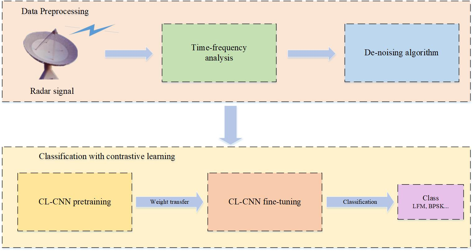
The CL–based model needs a deep network to extract the features of images, and as CNN is widely used in image classification for its excellent feature extraction performance, it is employed in our CL–based network. The newly constructed network is called CL–CNN, and its architecture is shown in Figure 1. There are mainly three parts in the pretraining stage, which are the stochastic data augmentation module, the encoder and the projection head. In the fine–tuning stage, the projection head is discarded, and the classification head is added after the encoder.
These parts play different roles in radar signal modulation classification. In the pretraining stage, the stochastic data augmentation module is mainly used for producing positive sample pairs and negative sample pairs, the encoder extracts representative features from data examples, the projection head maps representations to the space where the contrastive loss is applied and the classification head makes the final decision for modulation classification in the fine–tuning stage.
The training process of CL–CNN includes two steps, pretraining and fine–tuning, as shown in Figure 1. In the pretraining step, the encoder and the projection head are pretrained with unlabeled augmented data to map the original time–frequency images into low–dimensional representations. The aim is to minimize the contrastive loss and make the features of the anchor data more similar to that of the positive data and more dissimilar to that of the negative ones.
In the fine–tuning step, the weight of the encoder is saved, and a classification head is built after it. The encoder and classification head are together trained with labeled data. The latent representation obtained from the last step has already learned the intrinsic information from the unlabeled data examples, so only a small number of labeled data is needed to fine–tune the model.

4.2. De–Noising Algorithm

A time–frequency analysis can reduce noise to some extent, but some noise still remains, especially at low SNRs. Denoising algorithms can be used to further reduce the noise in the time–frequency images. Two–dimensional Wiener filtering is one of the effective denoising algorithms that can adjust the effect of the filter according to the local variance of the image. A detailed introduction to 2D Wiener filtering is given below, and more details can be found in [46].
Consider a 1D gray–scaled image of a × b pixels with value matrix H a × b , and the value of each pixel is denoted as H ( i , j ) , i = 1 , 2 , , a , j = 1 , 2 , , b . The size of a filter neighborhood is a ^ × b ^ , and the mean μ ^ and variance σ ^ 2 of each pixel of the neighborhood can be calculated by the following equations:
μ ^ = 1 a ^ b ^ i , j β ^ H ( i , j ) σ ^ 2 = 1 a ^ b ^ i , j β ^ H 2 ( i , j ) μ ^ 2 H ^ ( i , j ) = μ ^ + σ ^ 2 + σ N 2 σ ^ 2 [ H ( i , j ) μ ^ ]
where H ^ ( i , j ) is the filtered pixel of H ( i , j ) and σ N 2 the variance of the noise.

4.3. Data Augmentation

In this paper, the data augmentation part is implemented by random resized crop, horizontal flip and Gaussian noise. These data augmentation methods increase the diversity of the positive and negative sample pairs. In detail, ‘random resized crop’ randomly crops an area on the original image and then resizes it into a given size, and ‘horizontal flip’ flips the image horizontally. These two data augmentation methods enhance the generalization ability of the model. ‘Gaussian noise’ adds zero mean Gaussian noise to the original image, which distorts the high–frequency features and enhances the learning ability of the neural network.
Suppose the batch size of the input data is N ; after data augmentation, each input sample x k in this batch forms a positive pair x ^ 2 k 1 , x ^ 2 k , and all remaining 2 N 1 samples in this batch are used to form negative pairs.

4.4. Encoder

The encoder is a deep network used for feature extraction. The network cannot be too deep, as the gradient disappearance problem will appear, and the parameters of the previous layer cannot be trained effectively. The residual network (ResNet) is composed of some residual blocks, and it can alleviate the training difficulty by shortcut connections. The output of ResNet can be obtained by summing the output and input of multiple cascaded convolutional layers [47]. There is a Rectified Linear Unit (ReLU) nonlinear activation function after each residual block. The structure of the residual block is shown in Figure 2. It can be seen that the residual block mainly contains two 3 × 3 convolution layers (Conv), two batch normalization layers (BN) and three nonlinear activation function layers. For the input x ^ i , suppose h i is the final output of the residual block, and it is the sum of the forward neural network H x ^ i and x ^ i , i.e., h i = H x ^ i + x ^ i .

4.5. Projection Head

The projection head is composed of two fully connected layers, which maps the output of the encoder to a low–dimensional feature space and helps identify the invariant features of each input. The processing steps are listed as follows.
(1)
Calculate the output of the projection head for each input h i .
z i = W 2 σ W 1 h i
where i = 1 , 2 , , 2 N , N is the batch size, W 1 and W 2 are the weights of the two fully connected layers and σ is the ReLU nonlinear activation function.
(2)
Calculate the cosine similarity for each output of the projection head.
sim z i , z j = z i T z j z i z j
where is the l 2 norm, and T is the conjugate transposition operation.
(3)
Calculate the average normalized temperature–scaled cross–entropy loss.
L ¯ = 1 2 N k = 1 N L 2 k 1 , 2 k + L 2 k , 2 k 1 L ( i , j ) = log exp sim z i , z j / ξ k = 1 2 N I [ k i ] exp sim z i , z k / ξ
where ξ is the adjustable temperature parameter, and I [ k i ] 0 , 1 is an indicator function. The value of the indicator is 0 if and only if k = i ; otherwise, it is 1.
(4)
Update the parameters of the encoder and projection head to minimize the loss L ¯ .

4.6. Classification Head and Focal Loss Function

In the classification stage, as the parameters of the encoder have been pretrained and the projection head has been discarded, two fully connected layers are included to make the final decision on the modulation type.
In general, the cross–entropy loss function is widely used in the classification stage. However, the cross–entropy loss treats all the samples equally and does not differentiate the complicated samples and simple ones. Therefore, the classification performance may degrade due to the difficulty imbalance problem. The cross–entropy loss function can be written as
CE p = log p
where p 0 , 1 is the model’s estimated probability for the ground–truth class.
Compared with the cross–entropy loss function CE p , the focal loss function can be seen as the cross–entropy loss function with an extra adjustable parameter, which can be written as
FL ( p ) = ( 1 p ) γ log ( p )
where γ is an adjustable hyperparameter.
Normally, the probability p is small for difficult samples, which is p 0 and 1 p γ 1 ; as a result, the focal loss does not change significantly. On the contrary, the probability p of simple samples is large, so the contribution of this probability to the total loss is small. Employment of the focal loss in the classification head solves most of the difficulty imbalance problems and further improves the classification performance.

5. Simulations and Analyses

In this section, the classification performance of the CL–CNN model is compared with three deep models and two traditional methods, which are AAMC–DCNN, CNN–Xia, ResNet, SVM and KNN. The benchmark datasets are introduced, and the implementation details are introduced briefly. Then, the parameter settings of the CL–CNN model are studied, and the classification results are presented. All the simulation results are obtained by 50 trials.

5.1. Datasets

Simulations are conducted using two datasets, which contain nine types of radar intra–pulse signals shown in Table 1 and are contaminated by Gaussian white noise and impulsive noise, separately. The parameter settings of the signals are listed in Table 2, where U denotes the uniform random distribution of data in a fixed interval; represents a random parameter set and f s , f c , B , N s , L c , N c c , N g , M and ρ represent the sampling frequency, carrier frequency, bandwidth, number of samples, length of barker, number of carrier cycles in a single–phase symbol, number of segments, number of frequency steps and number of subcodes in a code, respectively.
The time–frequency images of four types of signals, i.e., LFM, two PSK and Frank, under white Gaussian noise and impulsive noise are shown in Figure 3, respectively. There are clear differences between the signal images under different types of noise.

5.2. Comparisons with Deep Models and Traditional Methods

Three types of deep models and two types of traditional methods are compared with the CL–CNN model for radar intra–pulse signal modulation classification. Furthermore, the CL–CNN–CE model using the cross–entropy loss function is also considered as one comparison model, which is different from the CL–CNN model using the focal loss function. For all the deep models, the softmax activation function is used in the last layer, and the Adam optimizer and cross–entropy loss function are applied in the deep models. The details of the deep models and traditional methods are listed in Table 3.
The AAMC–DCNN model is similar to DenseNet, but it has a dense–connection mechanism [28]. A two–stage training strategy is adopted for the model. In the first stage, the model is pretrained on the widely used ImageNet dataset. In the second stage, the pretrained model is fine–tuned for classification using the time–frequency images of our datasets.
The CNN–Xia model contains several convolution layers, maxpooling layers and fully connected layers [18]. There is a maxpooling layer after each convolution layer. Two fully connected layers and a dropout layer are added after the convolutional layers.
The ResNet model is a well–known deep convolutional neural network. The shortcut connections in the model can alleviate training difficulties in deeper networks without introducing either extra parameters or computational complexity. Many successful applications have been made using this model in modulation classification [48,49,50].
The SCRNN (Sequential Convolutional Recurrent Neural Network) model combines the speed and lightness of the CNN and temporal sensitivity of RNN [51]. It can be divided into three parts: the first part contains two convolutional layers with 128 filters and ReLU activation functions, the second part is two 128–unit LSTM layers with ReLU activation functions and the last part is a dense layer.
The SVM [52] maps the input data into a high–dimensional feature space, where a linear decision surface is constructed. Different types of classes are located on different sides of the decision surface.
The KNN (K–Nearest Neighbor) follows the nearest decision rule and assigns an unclassified sample point to the nearest classified set [53].

5.3. Implementation Details

For the first dataset, 5000 samples of each type of signals are produced for pretraining, while 85 and 1500 samples of each type of signals are produced for the fine–tuning and test, respectively. All of them are affected by Gaussian white noise. For the second dataset, 85 and 1500 samples of each type affected by impulse noise are produced to fine–tune and test the generalization ability of contrastive learning, respectively. The implementation details for the models and methods are shown in Table 4.
The Adam optimizer with a learning rate of 0.001 is utilized. All the trainings and predictions are implemented in Pytorch.

5.4. Parameter Analyses

As the classification accuracy varies with the parameter settings, it is necessary to find the optimal parameters for the CL–CNN model. The impact of the parameter settings of the CL–CNN model is investigated below, including the adjustable parameter γ , the batch size N and the number of CNN layers.
Figure 4 shows how the adjustable parameter γ affects the classification accuracy. The value of γ represents how much attention the model pays to difficult samples. A large γ leads to a poor classification performance, which means that the model focuses too much on those samples. On the other hand, a small γ also leads to a poor performance, which implies that the difficulty imbalance problem cannot be solved effectively, which degrades the performance of the model. It can be seen that the model with γ = 0.1 gives the best performance, and the difficulty imbalance problem can be solved to some extent by adjusting this parameter.
The results by different batch sizes N are shown in Table 5, which indicates that the classification performance with batch size 32 is the best. Normally, a larger batch size will bring a better classification performance, but the performance will degrade when the batch size exceeds the threshold value [54].
The simulation results for different numbers of layers are shown in Table 6, which indicates that the classification performance of 34 layers is the best, with a running time of 7.72 s. Normally, a larger number of layers will increase the generalization ability and bring a better classification performance, but the performance will degrade due to the overfitting problem when the number of layers is too large.

5.5. Performance Comparisons

The classification results are presented in this subsection, including CL–CNN and CL–CNN–CE, four deep models and two traditional methods. In addition, CL–CNN–WP is also considered in the comparison, which has the same structure as CL–CNN– CE and is directly fine–tuned without pretraining. All the deep models and traditional methods are configured in their best performance. The first simulation tests the effect of denoising, the second to fifth simulations test the feature extraction ability of contrastive learning, the sixth and seventh simulations test the generalization ability and the last one is the statistical analysis. For all simulations, 1500 samples of each signal type are used for the test, and 15–85 samples of each signal type are used for fine–tuning.
In the first simulation, the performances of CL–CNN using filtered and unfiltered images as input are shown in Table 7. The sample size for each class is set as 55. It can be seen that the method using filtered images achieves 3% to 4% more classification accuracy improvement than the one using unfiltered images at low SNRs. The comparison results indicate that the denoising algorithm is effective in reducing the effect of noise.
In the second simulation, the performances of CL–CNN, CL–CNN–CE and CL–CNN–WP are compared, and the results are shown in Table 8. It can be seen that CL–CNN achieves 1% to 2% classification rate improvement compared with CL–CNN–CE, which implies that the focal loss function effectively solves the difficult imbalance problem to further improve the classification performance. The performance of CL–CNN–WP is the worst, especially in the case of insufficient samples. It indicates that the pretraining greatly improves both the feature extraction ability and classification performance with a limited number of samples.
In the third simulation, the performance of CL–CNN with different sample sizes for each class and SNR is presented, and the results are shown in Table 9. The sample size for each type of signal increases from 15 to 85 with an interval of 10. It can be concluded that the proposed model exhibits good performance in a different number of samples, and the classification accuracy improves as the number of samples increases or SNR increases. When the SNR and sample size for each class are equal to or greater than −1 dB and 55, separately, the classification accuracy is more than 90%.
In the fourth simulation, the classification results of the deep models and traditional methods with the sample size per class 15 are shown in Table 10. It can be seen that CL–CNN achieves much better classification accuracy than the other deep models and traditional methods, which indicates that CL improves the feature extraction ability of the proposed model. As the deep models, CNN–Xia, AAMC–DCNN and ResNet are based on time–frequency images, while SCRNN, SVM and KNN are based on signal sequences, the classification performances of the first three models are clearly better than those of the other three. As the architecture of AAMC–DCNN is complex and the number of samples is very small, the overfitting problem may cause degradation to its performance, and as a result, CNN–Xia performs better with a simple structure. The signal sequence–based solutions show poor performances due to low discriminating inputs; while, among them, the performance of SVM is better than that of KNN.
In the fifth simulation, the models with the sample sizes per class 55 are tested, and the results are shown in Table 11. Although the sample size per class increases compared with that in the fourth simulation, CL–CNN still performs the best. It outperforms CNN–Xia and ResNet by nearly 4% for the whole SNR range. The performance of AAMC–DCNN has some improvement, which is comparable to CL–CNN with the SNR equal to or greater than 0 dB. The performance of SCRNN does not improve obviously when the sample size per class increases, as it may still suffer from the overfitting problem. The performance of KNN is better than that of SVM with an increased sample size for each class.
The confusion matrix is an important visual tool to compare the predicted results, which is provided in the sixth simulation. Confusion matrices of CL–CNN at various SNRs are presented in Figure 5, where each column represents the predicted modulation class, and each row represents the real modulation class, and the numerical value on each grid denotes the classification probability of the corresponding modulation class. It can be seen that the diagonals become sharper with an increasing SNR, which illustrates that a higher SNR brings a better classification accuracy. However, confusion between Frank and P3 exists when the SNR is equal to or is lower than −5 dB, as it is difficult to distinguish their modulation features at low SNRs.

5.6. Generalization Ability Test

In the following two simulations, the Gaussian noise–affected signals are used in the first pretraining stage, and the impulsive noise–affected signals are utilized in the fine–tuning stage. As SCRNN, SVM and KNN use the signal sequence as the input, their performance is very poor in the impulsive noise scenario, so they are not included in the comparison. The classification results are presented in Table 12 and Table 13 with the sample size for each class set as 15 and 55, separately. It can be seen that the proposed CL–CNN has the best performance in Table 12 and Table 13. Generally, the performance of CL–CNN using impulsive noise–affected signals in the fine–tuning stage does not degrade much compared with that using Gaussian noise, which indicates that the proposed CL–CNN has a good generalization ability.

5.7. Statistical Analysis with McNemar’s Test

McNemar’s test is employed to evaluate the statistical significance between the CL–CNN model and some other deep models, i.e., AAMC–DCNN, CNN–Xia and ResNet. McNemar’s test can be written as
z = s 12 s 21 s 12 + s 21
where s 12 is defined as the number of samples misclassified by model 1 but classified successfully by model 2, while the definition of s 21 is in contrast. A greater value of |z| means that two models have significant differences in performance.
Let CL–CNN be model 1 and AAMC–DCNN, CNN–Xia and ResNet be model 2, respectively. The values of |z| for different models are listed in Table 14. It can be seen that the performance of the CL–CNN model is statistically different from those of comparison models.

6. Conclusions

In this paper, a new deep learning–based model called CL–CNN was developed and applied to the radar intra–pulse modulation classification problem successfully. The impact of different parameter settings on its performance was examined to find the best configuration. Simulations were conducted using two datasets. As demonstrated by the results, the proposed model outperformed the other four deep models (AAMC–DCNN, CNN–Xia, ResNet and SCRNN) and two traditional methods (KNN and SVM) in terms of classification accuracy. From the simulation results, it can also be found that CL alleviates the overfitting problem encountered in few–shot learning and improves the feature extraction ability of the proposed model. Furthermore, the proposed model has a good generalization ability facing different noise types. Possible future work can focus on investigating more effective CL–based frameworks for radar intra–pulse modulation classification, which may further improve its performance.

Author Contributions

Conceptualization, J.C. and P.L.; methodology, X.C.; software, F.G.; validation, W.L.; formal analysis, J.C.; investigation, X.C.; resources, W.L.; data curation, F.G.; writing—original draft preparation, F.G. and writing—review and editing, J.C., X.C. and W.L. All authors have read and agreed to the published version of the manuscript.

Funding

This work was supported by the National Natural Science Foundation of China (No. 61805189 and 62176199) and the Fundamental Research Funds for the Central Universities (No. JB210201).

Data Availability Statement

Not applicable.

Acknowledgments

The authors would like to express their gratitude to the editors and the reviewers for their insightful comments.

Conflicts of Interest

The authors declare no conflict of interest.

References

  1. Gupta, M.; Hareesh, G.; Mahla, A.K. Electronic warfare: Issues and challenges for emitter classification. Def. Sci. J. 2011, 61, 228. [Google Scholar] [CrossRef] [Green Version]
  2. Qu, Z.; Mao, X.; Deng, Z. Radar signal intra-pulse modulation recognition based on convolutional neural network. IEEE Access 2018, 6, 43874–43884. [Google Scholar] [CrossRef]
  3. Yuan, S.; Li, P.; Wu, B.; Li, X.; Wang, J. Semi-supervised classification for intra-pulse modulation of radar emitter signals using convolutional neural network. Remote Sens. 2022, 14, 2059. [Google Scholar] [CrossRef]
  4. López-Risuño, G.; Grajal, J.; Sanz-Osorio, A. Digital channelized receiver based on time-frequency analysis for signal interception. IEEE Trans. Aerosp. Electron. Syst. 2005, 41, 879–898. [Google Scholar] [CrossRef]
  5. Zeng, D.; Zeng, X.; Cheng, H.; Tang, B. Automatic modulation classification of radar signals using the Rihaczek distribution and Hough transform. IET Radar Sonar Navig. 2012, 6, 322–331. [Google Scholar] [CrossRef]
  6. Fan, X.; Li, T.; Su, S. Intra-pulse modulation type recognition for pulse compression radar signal. J. Appl. Remote Sens. 2017, 11, 035018. [Google Scholar] [CrossRef]
  7. Kishore, T.R.; Rao, K.D. Automatic intra-pulse modulation classification of advanced LPI radar waveforms. IEEE Trans. Aerosp. Electron. Syst. 2017, 53, 901–914. [Google Scholar] [CrossRef]
  8. Wan, J.; Ruan, G.; Guo, Q.; Gong, X. A new radar signal recognition method based on optimal classification atom and IDCQGA. Symmetry 2018, 10, 659. [Google Scholar] [CrossRef] [Green Version]
  9. Lundén, J.; Koivunen, V. Automatic radar waveform recognition. IEEE J. Sel. Top. Signal Process. 2007, 1, 124–136. [Google Scholar] [CrossRef]
  10. Hinton, G.E.; Osindero, S.; Teh, Y.-W. A fast learning algorithm for deep belief nets. Neural Comput. 2006, 18, 1527–1554. [Google Scholar] [CrossRef]
  11. Krizhevsky, A.; Sutskever, I.; Hinton, G.E. Imagenet classification with deep convolutional neural networks. Adv. Neural Inf. Process. Syst. 2012, 25, 1097–1105. [Google Scholar] [CrossRef] [Green Version]
  12. Chen, X.; Zhang, H.; Song, J.; Guan, J.; Li, J.; He, Z. Micro-motion classification of flying bird and rotor drones via data augmentation and modified multi-scale cnn. Remote Sens. 2022, 14, 1107. [Google Scholar] [CrossRef]
  13. Wei, S.; Qu, Q.; Su, H.; Wang, M.; Shi, J.; Hao, X. Intra-pulse modulation radar signal recognition based on CLDN network. IET Radar Sonar Navig. 2020, 14, 803–810. [Google Scholar] [CrossRef]
  14. Wu, B.; Yuan, S.; Li, P.; Jing, Z.; Huang, S.; Zhao, Y. Radar emitter signal recognition based on one-dimensional convolutional neural network with attention mechanism. Sensors 2020, 20, 6350. [Google Scholar] [CrossRef] [PubMed]
  15. Wei, S.; Qu, Q.; Zeng, X.; Liang, J.; Shi, J.; Zhang, X. Self-attention bi-lstm networks for radar signal modulation recognition. IEEE Trans. Microw. Theory Tech. 2021, 69, 5160–5172. [Google Scholar] [CrossRef]
  16. Qu, Z.; Wang, W.; Hou, C.; Hou, C. Radar signal intra-pulse modulation recognition based on convolutional denoising autoencoder and deep convolutional neural network. IEEE Access 2019, 7, 112339–112347. [Google Scholar] [CrossRef]
  17. Gao, L.; Zhang, X.; Gao, J.; You, S. Fusion image based radar signal feature extraction and modulation recognition. IEEE Access 2019, 7, 13135–13148. [Google Scholar] [CrossRef]
  18. Xia, Y.; Ma, Z.; Huang, Z. Over-the-Air Radar Emitter Signal Classification Based on SDR. In Proceedings of the 2021 6th International Conference on Intelligent Computing and Signal Processing (ICSP), Xi’an, China, 9–11 April 2021. [Google Scholar]
  19. Jin, X.; Ma, J.; Ye, F. Radar Signal Recognition Based on Deep Residual Network with Attention Mechanism. In Proceedings of the 2021 IEEE 4th International Conference on Electronic Information and Communication Technology (ICEICT), Xi’an, China, 18–20 August 2021. [Google Scholar]
  20. Zhang, X.; Zhang, J.; Luo, T.; Huang, T.; Tang, Z.; Chen, Y.; Li, J.; Luo, D. Radar signal intrapulse modulation recognition based on a denoising-guided disentangled network. Remote Sens. 2022, 14, 1252. [Google Scholar] [CrossRef]
  21. Wang, Y.; Yao, Q.; Kwok, J.T.; Ni, L.M. Generalizing from a few examples: A survey on few-shot learning. ACM Comput. Surv. 2020, 53, 63. [Google Scholar] [CrossRef]
  22. Weiss, K.; Khoshgoftaar, T.M.; Wang, D. A survey of transfer learning. J. Big Data 2016, 3, 9. [Google Scholar] [CrossRef]
  23. Zhu, Y.; Chen, Y.; Lu, Z.; Pan, S.J.; Xue, G.-R.; Yu, Y.; Yang, Q. Heterogeneous Transfer Learning for Image Classification. In Proceedings of the Twenty-Fifth AAAI Conference on Artificial Intelligence, San Francisco, CA, USA, 7–11 August 2011. [Google Scholar]
  24. Zhou, J.; Pan, S.; Tsang, I.; Yan, Y. Hybrid Heterogeneous Transfer Learning through Deep Learning. In Proceedings of the AAAI Conference on Artificial Intelligence, Québec, Canada, 27–31 July 2014. [Google Scholar]
  25. Wang, Q.; Du, P.; Yang, J.; Wang, G.; Lei, J.; Hou, C. Transferred deep learning based waveform recognition for cognitive passive radar. Signal Process. 2019, 155, 259–267. [Google Scholar] [CrossRef]
  26. Guo, Q.; Yu, X.; Ruan, G. LPI radar waveform recognition based on deep convolutional neural network transfer learning. Symmetry 2019, 11, 540. [Google Scholar] [CrossRef] [Green Version]
  27. Lin, A.; Ma, Z.; Huang, Z.; Xia, Y.; Yu, W. Unknown radar waveform recognition based on transferred deep learning. IEEE Access 2020, 8, 184793–184807. [Google Scholar] [CrossRef]
  28. Si, W.; Wan, C.; Zhang, C. Towards an accurate radar waveform recognition algorithm based on dense CNN. Multimed. Tools Appl. 2021, 80, 1779–1792. [Google Scholar] [CrossRef]
  29. Chen, T.; Kornblith, S.; Norouzi, M.; Hinton, G. A Simple Framework for Contrastive Learning of Visual Representations. In Proceedings of the International Conference on Machine Learning, Online, 13–18 July 2020. [Google Scholar]
  30. He, K.; Fan, H.; Wu, Y.; Xie, S.; Girshick, R. Momentum Contrast for Unsupervised Visual Representation Learning. In Proceedings of the IEEE/CVF Conference on Computer Vision and Pattern Recognition, Washington, DC, USA, 14–19 June 2020. [Google Scholar]
  31. Tian, Y.; Krishnan, D.; Isola, P. Contrastive Multi-View Coding. In Proceedings of the European Conference on Computer Vision, Glasgow, UK, 23–28 August 2020. [Google Scholar]
  32. Liu, D.; Wang, P.; Wang, T.; Abdelzaher, T. Self-Contrastive Learning Based Semi-Supervised Radio Modulation Classification. In Proceedings of the MILCOM 2021–2021 IEEE Military Communications Conference (MILCOM), San Diego, CA, USA, 29 November–2 December 2021. [Google Scholar]
  33. Devlin, J.; Chang, M.-W.; Lee, K.; Toutanova, K. Bert: Pre-training of deep bidirectional transformers for language understanding. arXiv 2018, arXiv:1810.04805. [Google Scholar]
  34. Gidaris, S.; Singh, P.; Komodakis, N. Unsupervised representation learning by predicting image rotations. arXiv 2018, arXiv:1803.07728. [Google Scholar]
  35. Hou, S.; Shi, H.; Cao, X.; Zhang, X.; Jiao, L. Hyperspectral imagery classification based on contrastive learning. IEEE Trans. Geosci. Remote Sens. 2022, 60, 1–13. [Google Scholar] [CrossRef]
  36. Jing, L.; Tian, Y. Self-supervised visual feature learning with deep neural networks: A survey. IEEE Trans. Pattern Anal. Mach. Intell. 2020, 43, 4037–4058. [Google Scholar] [CrossRef]
  37. Zhang, R.; Isola, P.; Efros, A.A. Colorful Image Colorization. In Proceedings of the European Conference on Computer Vision, Amsterdam, The Netherlands, 8–16 October 2016. [Google Scholar]
  38. Shrivastava, A.; Gupta, A.; Girshick, R. Training Region-Based Object Detectors with Online Hard Example Mining. In Proceedings of the IEEE Conference on Computer Vision and Pattern Recognition, Las Vegas, NV, USA, 26 June–1 July 2016. [Google Scholar]
  39. Lin, T.-Y.; Goyal, P.; Girshick, R.; He, K.; Dollár, P. Focal Loss for Dense Object Detection. In Proceedings of the IEEE International Conference on Computer Vision, Honolulu, Hawaii, 22–25 July 2017. [Google Scholar]
  40. Tian, X.; Wu, D.; Wang, R.; Cao, X. Focal text: An Accurate Text Detection with Focal Loss. In Proceedings of the 2018 25th IEEE International Conference on Image Processing (ICIP), Athens, Greece, 7–10 October 2018. [Google Scholar]
  41. Chen, M.; Fang, L.; Liu, H. Fr-net: Focal Loss Constrained Deep Residual Networks for Segmentation of Cardiac MRI. In Proceedings of the 2019 IEEE 16th International Symposium on Biomedical Imaging (ISBI 2019), Venezia, Italy, 8–11 April 2019. [Google Scholar]
  42. Zimmermann, M.; Dostert, K. Analysis and modeling of impulsive noise in broad-band powerline communications. IEEE Trans. Electromagn. Compat. 2002, 44, 249–258. [Google Scholar] [CrossRef]
  43. Clavier, L.; Peters, G.W.; Septier, F.; Nevat, I. Impulsive noise modeling and robust receiver design. EURASIP J. Wirel. Commun. Netw. 2021, 2021, 13. [Google Scholar] [CrossRef]
  44. Zhou, Z.; Huang, G.; Chen, H.; Gao, J. Automatic radar waveform recognition based on deep convolutional denoising auto-encoders. Circuits Syst. Signal Process. 2018, 37, 4034–4048. [Google Scholar] [CrossRef]
  45. Wan, J.; Yu, X.; Guo, Q. LPI radar waveform recognition based on CNN and TPOT. Symmetry 2019, 11, 725. [Google Scholar] [CrossRef]
  46. Lim, J.S. Two-Dimensional Signal and Image Processing; Prentice-Hall: Englewood Cliffs, NJ, USA, 1990. [Google Scholar]
  47. He, K.; Zhang, X.; Ren, S.; Sun, J. Deep Residual Learning for Image Recognition. In Proceedings of the IEEE Conference on Computer Vision and Pattern Recognition, Las Vegas, NV, USA, 26 June–1 July 2016. [Google Scholar]
  48. OShea, T.J.; Roy, T.; Clancy, T.C. Over-the-air deep learning based radio signal classification. IEEE J. Sel. Top. Signal Process. 2018, 12, 168–179. [Google Scholar] [CrossRef] [Green Version]
  49. Qi, P.; Zhou, X.; Zheng, S.; Li, Z. Automatic modulation classification based on deep residual networks with multimodal information. IEEE Trans. Cogn. Commun. Netw. 2020, 7, 21–33. [Google Scholar] [CrossRef]
  50. Lu, X.; Tao, M.; Fu, X.; Gui, G.; Ohtsuki, T.; Sari, H. Lightweight Network Design Based on ResNet Structure for Modulation Recognition. In Proceedings of the 2021 IEEE 94th Vehicular Technology Conference (VTC2021-Fall), Online, 27–30 September 2021. [Google Scholar]
  51. Liao, K.; Zhao, Y.; Gu, J.; Zhang, Y.; Zhong, Y. Sequential convolutional recurrent neural networks for fast automatic modulation classification. IEEE Access 2021, 9, 27182–27188. [Google Scholar] [CrossRef]
  52. Cortes, C.; Vapnik, V. Support-vector networks. Mach. Learn. 1995, 20, 273–297. [Google Scholar] [CrossRef]
  53. Cover, T.; Hart, P. Nearest neighbor pattern classification. IEEE Trans. Inf. Theory 1967, 13, 21–27. [Google Scholar] [CrossRef]
  54. Keskar, N.S.; Mudigere, D.; Nocedal, J.; Smelyanskiy, M.; Tang, P.T.P. On large-batch training for deep learning: Generalization gap and sharp minima. arXiv 2016, arXiv:1609.04836. [Google Scholar]
Figure 1. Architecture of the CL–CNN model.
Remotesensing 14 05728 g001
Figure 2. Structure of the residual block.
Remotesensing 14 05728 g002
Figure 3. The time–frequency images: (a) LFM signal under Gaussian noise, (b) BPSK signal under Gaussian noise, (c) Frank signal under Gaussian noise, (d) LFM signal under impulsive noise, (e) BPSK signal under impulsive noise, (f) Frank signal under impulsive noise, (g) filtered image of LFM signal under Gaussian noise and (h) filtered image of LFM signal under impulsive noise.
Remotesensing 14 05728 g003
Figure 4. Classification performance of the CL−CNN model with different γ (the sample size per class is 55).
Remotesensing 14 05728 g004
Figure 5. Confusion matrices of the CL–CNN model at different SNRs: (a) SNR -10dB, (b) SNR-5dB, (c) SNR 0dB.
Remotesensing 14 05728 g005
Table 1. The instantaneous phase representation of nine types of radar signals.
Modulation TypeParameter ϕ k
LFM f c
μ
2 π f c k ± μ 2 k 2
BPSK f c
θ
2 π f c k + θ , θ { 0 , π }
T1 m
T
n
2 π f c k + mod 2 π n INT ( m k j T ) j n T , 2 π , j = 1 , 2 , , k 1
T2 m
T
n
2 π f c k + mod 2 π n INT ( m k j T ) 2 j m + 1 T n 2 , 2 π , j = 1 , 2 , , k 1
Frank M 2 π f c k + 2 π ( i 1 ) ( j 1 ) / M , i = 1 , 2 , , M , j = 1 , 2 , , M
P1 M 2 π f c k π [ M ( 2 j 1 ) ] [ ( j 1 ) M + ( i 1 ) ] / M , i = 1 , 2 , , M , j = 1 , 2 , , M
P2 M 2 π f c k π [ 2 i 1 M ] [ 2 j 1 M ] / 2 M , i = 1 , 2 , , M , j = 1 , 2 , , M
P3 N c 2 π f c k + π ( i 1 ) 2 / N c , i = 1 , 2 , , N c
P4 N c 2 π f c k + π ( i 1 ) 2 / N c π ( i 1 ) , i = 1 , 2 , , N c
Table 2. The parameter settings of nine types of radar intra–pulse signals.
Modulation TypeParameterRanges
f s 200 MHz
LFM f c
B
N s
U 3 f s / 20 , f s / 5
U f s / 20 , f s / 10
U ( 500 , 1000 )
BPSK L c
f c
N c c
{ 7 , 11 , 13 }
U 3 f s / 20 , f s / 5
{ 20 , 21 , 22 , 23 }
T1, T2 f c
N g
N
U 3 f s / 20 , f s / 5
{ 4 , 5 , 6 }
U ( 500 , 1000 )
Frank, P1 f c
N c c
M
U 3 f s / 20 , f s / 5
{ 4 , 5.6 }
{ 5 , 6 , 7 , 8 }
P2 f c
N c c
M
U 3 f s / 20 , f s / 5
{ 4 , 5 , 6 }
{ 6 , 8 }
P3, P4 f c
N c c
ρ
U 3 f s / 20 , f s / 5
{ 4 , 5.6 }
{ 36 , 49 , 64 }
Table 3. The details of the deep models and traditional methods.
ModelInputCross–Entropy LossFocal LossTransfer LearningContrastive Learning
CL–CNNTime–frequency imagesNoYesNoYes
CL–CNN–CETime–frequency imagesYesNoNoYes
AAMC–DCNNTime–frequency imagesYesNoYesNo
CNN–XiaTime–frequency imagesYesNoNoNo
ResNetTime–frequency imagesYesNoNoNo
SCRNNSignal sequencesYesNoNoNo
SVMSignal sequences----
KNNSignal sequences----
Table 4. The implementation details of the deep models and traditional methods.
ModelPretrainingFine–TuningDirect Training
CL–CNNDataset1: 5000 samples for each classDataset 1: 15–85 samples for each class
Dataset 2: 15–85 samples for each class
No
AAMC–DCNNImageNet
CNN–XiaNoNoDataset 1: 15–85 samples for each class
Dataset 2: 15–85 samples for each class
ResNet
SCRNNNoNoDataset 1: 15–85 samples for each class
SVM--
KNN
All of the models and methods are tested with 1500 samples for each class.
Table 5. Classification performance of the CL–CNN model at different batch sizes with −5 dB SNR and the sample size of each class being 55.
Batch Size8163264128
Accuracy(%)78.4879.7082.0978.7176.19
Table 6. Results of the CL–CNN model with a different number of layers with −5 dB SNR and the sample size for each class being 55.
Layer Number183450101
Accuracy(%)79.3282.0975.9672.54
Time cost * (s)6.677.729.5213.42
* The running time of the whole test samples.
Table 7. Classification performance of CL–CNN using filtered and unfiltered time–frequency images based on the first dataset.
InputSNR(dB)
−10−9−8−7−6−5−4−3−2−10
Filtered images53.1159.8563.7069.9775.9582.0986.1288.3193.0593.7294.02
Unfiltered images48.97 54.83 60.04 66.19 70.81 77.39 82.18 85.53 90.13 91.20 93.42
Table 8. Classification performance of the CL–CNN, CL–CNN–CE and CL–CNN–WP models at −5 dB SNR.
ModelSample Size for Each Class
1525354555657585
CL–CNN63.6172.5776.6479.0982.0983.6984.7487.47
CL–CNN–CE62.2469.4975.1177.6280.2781.2282.5486.14
CL–CNN–WP52.4162.7463.3964.5068.6673.7378.6983.73
Table 9. Classification performance of the CL–CNN model in varying sample sizes for each class and SNR.
SNR−10 dB−9 dB−8 dB−7 dB−6 dB−5 dB−4 dB−3 dB−2 dB−1 dB0 dB
Size
1537.7342.5747.6352.2156.5863.6167.4370.8276.1383.6385.36
2537.9445.6750.7754.3860.4172.5774.1975.9178.6985.7186.92
3542.5446.1554.8157.8068.6076.6476.6380.7283.5587.3587.47
4546.7848.9157.4662.3671.9279.0981.4982.3785.9290.6391.19
5553.1159.8563.7069.9775.9582.0986.1288.3193.0593.7294.02
6553.6260.4663.3070.4476.4383.6986.6888.5693.2293.3093.44
7553.2360.7463.6971.3976.8784.7486.8488.4893.1993.6693.94
8557.0364.8668.9274.7882.5187.4790.9590.4293.5794.5694.79
Table 10. Classification performances of the deep models, and the traditional methods with the sample size for each class being 15 based on the first dataset.
ModelSNR (dB)
−10−9−8−7−6−5−4−3−2−10
CL–CNN37.7342.5747.6352.2156.5863.6167.4370.8276.1383.6385.36
AAMC–DCNN 30.2932.0334.7437.9041.5443.5947.3050.8958.6469.3475.06
CNN–Xia 34.3537.2143.1247.4351.4657.2561.1962.5270.5975.6781.61
ResNet 33.9435.2737.8042.4748.9052.5054.9657.2565.2670.8076.94
SCRNN 12.7313.5313.0614.1016.0215.1917.1117.1518.6120.0820.01
SVM 13.6114.5114.3716.8917.7017.3918.5318.1619.2120.8021.45
KNN13.0512.9113.8314.7614.9416.1716.6217.2717.1417.3217.33
Table 11. Classification performances of the deep models and the traditional methods, with the sample size for each class being 55 based on the first dataset.
ModelSNR(dB)
−10−9−8−7−6−5−4−3−2−10
CL–CNN53.1159.8563.7069.9775.9582.0986.1288.3193.0593.7294.02
AAMC–DCNN47.8953.1759.9164.4868.2173.2279.2183.5490.3591.2392.37
CNN–Xia49.1655.0660.4965.2269.3375.3078.9683.9090.9391.4591.63
ResNet50.0756.2661.1165.9170.2577.3681.5984.6391.5993.4293.96
SCRNN14.8113.7316.5117.2318.0419.3319.0322.3023.9426.8629.36
SVM16.5217.0519.1021.2521.8323.4524.9525.9826.8429.6229.13
KNN14.7115.5417.2120.5222.6324.426.3227.6229.6533.3733.05
Table 12. Generalization ability test with the sample size for each class being 15.
ModelSNR (dB)
−10−9−8−7−6−5−4−3−2−10
CL–CNN36.8441.8247.3051.5555.8562.7166.6770.1875.8083.1984.90
AAMC–DCNN 29.6531.6334.1537.3840.9643.1346.7350.2258.2868.7874.51
CNN–Xia 33.7136.7142.6046.9251.0856.8260.6762.0170.3575.2081.12
ResNet 33.4734.7337.2241.8348.2952.0354.3356.7364.6970.3176.52
Table 13. Generalization ability test with the sample size for each class being 55.
ModelSNR(dB)
−10−9−8−7−6−5−4−3−2−10
CL–CNN52.4959.2763.1969.3975.5981.5185.7687.8992.4493.2993.59
AAMC–DCNN47.3252.7859.3264.1867.7172.6878.7483.0289.8790.7591.65
CNN–Xia48.7854.4460.0864.8068.7873.6478.5280.4090.5390.9191.43
ResNet49.5355.7260.7965.4969.7276.8081.0984.2991.0692.8993.52
Table 14. The values of |z| with −5 dB SNR and the sample size for each class being 55.
AAMC–DCNNCNN–XiaResnet
|z|24.3621.0915.80
Publisher’s Note: MDPI stays neutral with regard to jurisdictional claims in published maps and institutional affiliations.

