Comparison on Quantitative Analysis of Olivine Using MarSCoDe Laser-Induced Breakdown Spectroscopy in a Simulated Martian Atmosphere

Abstract

A Mars Surface Composition Detector (MarSCoDe) instrument mounted on Zhurong rover of Tianwen-1, adopts Laser-Induced Breakdown Spectroscopy (LIBS), with no sample preparation or dust and coatings ablation required, to conduct rapid multi-elemental analysis and characterization of minerals, rocks and soils on the surface of Mars. To test the capability of MarSCoDe LIBS measurement and quantitative analysis, some methods of multivariate analysis on olivine samples with gradient concentrations were inspected based on the spectra acquired in a Mars-simulated environment before the rover launch in 2020. Firstly, LIBS spectra need preprocessing, including background subtraction, random signal denoising, continuum baseline removal, spectral drift correction and wavelength calibration, radiation calibration, and multi-channel spectra subset merging. Then, the quantitative analysis with univariate linear regression (ULR) and multivariate linear regression (MLR) are performed on the characteristic lines, while principal component regression (PCR), partial least square regression (PLSR), ridge, least-absolute-shrinkage-and-selection-operator (LASSO) and elastic net, and nonlinear analysis with back-propagation (BP) are conducted on the entire spectral information. Finally, the performance on the quantitative olivine analyzed by MarSCoDe LIBS is compared with the mean spectrum and all spectra for each sample and evaluated by some statistical indicators. The results show that: (1) the calibration curve of ULR constructed by the characteristic line of magnesium and iron indicates the linear relationship between the spectral signal and the element concentration, and the limits of detection of forsterite and fayalite is 0.9943 and 2.0536 (c%) analyzed by mean spectra, and 2.3354 and 3.8883 (c%) analyzed by all spectra; (2) the R² value on the calibration and validation of all the methods is close to 1, and the predicted concentration estimated by these calibration models is close to the true concentration; (3) the shrinkage or regularization technique of ridge, LASSO and elastic net perform better than the ULR and MLR, except for ridge overfitting on the testing sample; the best results can be obtained by the dimension reduction technique of PCR and PLSR, especially with PLSR; and BP is more applicable for the sample measured with larger spectral dataset.

1. Introduction

The Mars Surface Composition Detector (MarSCoDe) is a remote sensing instrument suite mounted on the front deck of the Zhurong rover, in China’s first Mars exploration mission Tianwen-1. MarSCoDe adopts Laser-Induced Breakdown Spectroscopy (LIBS), Short Wave InfRared (SWIR) spectroscopy and Telescopic Micro-Imager (TMI) [1] to implement a partial, detailed, in situ investigation of the elements, minerals, and rocks of the roving area [2,3,4,5]. LIBS, a direct spectrochemical analytical method based on atomic emission, focuses a high-energy pulsed laser on a sample (i.e., solid, liquid, aerosol, and gaseous) to heat, melt, vaporize, and then generate an ionized and short-lived plasma (contains atoms, ions, and free electrons) [6,7]. The photons emitted at wavelengths that are unique to each element are resolved by the spectrometer to form a spectrum [8]. The rich emission-specific lines, indicating the chemical composition of the sample, can be used to identify and quantify the concentration of major, minor, and even trace elements [9].

LIBS has several well-known advantages, such as multi-elemental analysis without sample preparation, the active removal of dust and coatings and the effectiveness of in situ and remote detection, even under the extreme conditions of pressure and temperature and hazardous pollutants [6,10]. From the first observed optical emission with laser impact in 1962 [11], it has been recognized as a powerful tool for elemental composition analysis and used in remote detection since the late 1980s [12]. The observed distance has increased to as far as 180 m in some experiments [13]. Using planetary surfaces was then suggested [14], and the first occasion was integrated onto a rover in a field setting [15]. Therefore, it is well suited for planet exploration, such as the moon, Mars, and Venus [9], to provide the geochemical analysis of rocks and soils. The Curiosity rover’s ChemCam was the first remote LIBS to detail Martian geochemistry with a stand-off distance of 1.5–7 m [16]. The components of the ChemCam were described by Wiens et al. [17], its performance and science specification were reported in [18], and ground data-processing techniques (including dark subtraction, denoising, continuum removal, spectral calibration, radiation calibration, etc.) were used to produce clean spectra [10,19]. The Perseverance rover’s SuperCam also uses the remote LIBS in the Mars 2020, the components and science objectives were presented in [20,21], and its preprocessing and some quantitative analyses were introduced in [22].

In practice, most of quantitative analysis methods of LIBS have been applied to various research fields based on linear algebra in order to establish the best relationship between the measured signal and the analyte concentration. The simplest case uses univariate analysis to model the single spectral peak with the elemental content, but it is defected in the interference, self-absorption [23], and matrix effect [24]. Meanwhile, multivariate analysis can provide stable models when the samples have highly variable matrix and composition [25]. There are more multivariate linear methods, e.g., ordinary multi-linear regression (MLR), principal component regression (PCR) [26], partial least square regression (PLSR) [10,27,28,29], least-absolute-shrinkage-and-selection-operator (LASSO) [28], elastic net, sparse multivariate-regression-with-covariance-estimation (MRCE) [30,31], etc. Some methods use artificial neural networks (ANN) [32,33] to account for the possible nonlinear relationship. Nevertheless, quantifying the material content based on the LIBS spectra is a difficult task, especially for stand-off detection. At present, more demonstrations on these multivariate quantitative chemometric strategies have been performed by the ChemCam team [10,34] and tested on SuperCam [22]. Whether these methods can be used in MarSCoDe needs to be systematically tested and compared.

To test the capability of MarSCoDe LIBS measurement and quantitative analysis and try to avoid the matrix effect, some olivine samples with gradient concentrations were prepared and the experiments in a simulated Martian atmosphere were conducted before the launch. This paper focuses on the procedure of preprocessing and quantitative analysis on the MarSCoDe LIBS with the commonly univariate linear regression (ULR), the multivariate analysis of ordinary MLR, PCR, PLSR, Ridge, LASSO and elastic net, and the ANN analysis of back-propagation (BP). The performance of these methods is compared by the mean spectrum and all the spectra for each sample and evaluated with some statistical indicators (such as R², mean absolute error, standard error, and root mean square error). Firstly, the performance of the instrument, the sample preparation and Mars simulation experiment are introduced (in Section 2.1). Secondly, the methods of ground data-preprocessing and some quantitative analyses are presented (in Section 2.2 and Section 2.3). Then the performance on the quantification of olivine with MarSCoDe LIBS has been compared and evaluated (in Section 3). Finally, some conclusions are discussed (in Section 4).

2. Materials and Methods

2.1. Test Samples and Experiment Environment

The wide use of LIBS is to conduct qualitative and quantitative analysis by comparing the examined spectra and the reference spectra with a known material concentration. The LIBS spectra of a complex sample containing several elements may have overlapping spectral lines and the characteristic emission lines usually need high spectral resolution to cover a range from 240 to 850 nm [17,35,36]. Some samples can be prepared and placed in a simulated Martian atmosphere and measured by the LIBS system of MarSCoDe.

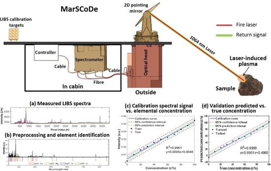
2.1.1. Instrument Description and Simulated Experiment

MarSCoDe is one of six scientific payloads and mounted on the front deck of the Zhurong rover, launched on 23 July 2020 and landed at the candidate site of the Utopia Planitia on 15 May 2021. It utilizes a LIBS to provide element compositional information with active spectroscopy over 240–850 nm, an Acousto-optic Tunable Filter (AOTF) to collect reflected information with passive SWIR over 800–2400 nm, and a TMI to capture sample texture and morphology image to perform the in situ detection with a stand-off distance of 1.6–7 m. With the help of a two-dimensional (2D) pointing mirror, the remote instrument can point small observation footprints with fine-scale sampling and perform the line scan on rock targets and depth profiling through surface coating. These can be used for sample classification, composition quantitative, and even 3D characterization.

Figure 1a shows the main units of the MarSCoDe instrument suite, and

Table 1. Main parameters of MarSCoDe LIBS.

Items	Values
Stand-off distance	1.6–7 m
Laser type	Nd:YAG
Laser wavelength	1064 nm
Pulse width	4 ns
Laser energy	23 mJ
Pulse frequency	1, 2, 3 Hz
Pulse energy density	200 MW/mm2 @ 2 m32 MW/mm2 @ 5 m
Spectral range	240.00–850.00 nm
Spectral sampling interval	0.067 nm @ 240–340 nm
	0.132 nm @ 340–540 nm
	0.203 nm @ 540–850 nm

lists the main technical parameters of LIBS. The composition and performance of the equipment have been detailed in the literature [1]. There are three array CCDs with 2048 pixels to record the LIBS spectral response. Selected 1800 pixels among the CCD to correspond to three channels with a spectral sampling interval of 0.067, 0.132, and 0.203 nm, respectively. The LIBS spectrometer also has a sufficient sensitivity to collect the reflectance spectroscopy over the same spectral range, conducted in passive mode as a by-product of the LIBS. This measurement is typically used as a background after laser shots to assist in the calibration of LIBS.

These samples were placed into a vacuum chamber measured in a simulated Martian environment, as illustrated in Figure 1. The chamber was filled with the simulated Martian atmospheric composition gases with Ar of 1.6%, N₂ of 2.7% and CO₂ of 95.7%, at the pressure of 700 ± 50 Pa, with a room temperature. Considering most of the on-board detection targets may be located at 3 m and obtained with the ideal signal–noise ratio, the LIBS spectra were recorded by the MarSCoDe LIBS with a laser-to-sample distance of approximately 3 m on 9 October 2019. The laser was emitted at a frequency of 3 Hz after an autofocus was performed in the center of each sample. One location of each sample was shot by 60 consecutive laser pulses and hence 60 LIBS spectra were recorded, another 60 passive spectra without the laser shot were collected and their on-board mean was regarded as the background. All these spectra were measured with an integration time of 1 ms.

2.1.2. Sample Pretreatment and Component Content

Although one of the most advantages of LIBS is no need for sample preparation, the pretreatment of samples could improve the quality of LIBS spectra. For the solid samples, it usually directly presses the homogeneous powder of standard material into pellet. The olivine is a silicate of magnesium and iron, an ultramafic and the main igneous rock of Mars. A chemical composition of the olivine is usually the end member between magnesium olivine (Mg₂SiO₄), referred to as forsterite (Fo), and iron rich olivine (Fe₂SiO₄), referred as fayalite (Fa). The different content indicates the different physical conditions in the geological formation. In natural igneous rock, Mg and Fe are generally oxides, and they can also be used to simulate the Fo and Fa. For the synthesis of Mg₂SiO₄, MgO and SiO₂ were mixed at a ratio of 2 to 1, and for Fe₂SiO₄, Fe₂O₃ and SiO₂ were mixed at a ratio of 1 to 1. The chemical formula of the final magnesium olivite terminal mineral (Mg₂SiO₄) shares the composition (2(MgO) + SiO₂). The chemical formula of the final iron olivite terminal mineral (Fe₂SiO₄) and the composition scheme (Fe₂O₃ + SiO₂) are slightly different, but due to oxygen elements in the air, oxygen elements are ignored in the analysis. To obtain olivine with a gradient content of Mg and Fe, homogeneous well-ground oxide mixtures with different desired ratios of MgO, Fe₂O₃, and SiO₂ were prepared as a stoichiometric composition.

To investigate the accuracy of the quantitative chemical analysis of these chemical composition with MarSCoDe LIBS, there are eleven samples with gradient concentrations from 0% to 100% mixed as the training set to establish the calibration model, and three samples at concentrations of 25%, 55%, and 75% mixed as a testing set to validate the calibration model,

Table 2. End-number for the samples and mixtures.

Samples		Mg2SiO4 (Fo)	Fe2SiO4 (Fa)	MgO	Fe2O3	SiO2
		Content/c%		Proportional Coefficient of Moles Content
Training	A01	0	100	0	100	100
	A02	10	90	20	90	100
	A03	20	80	40	80	100
	A04	30	70	60	70	100
	A05	40	60	80	60	100
	A06	50	50	100	50	100
	A07	60	40	120	40	100
	A08	70	30	140	30	100
	A09	80	20	160	20	100
	A10	90	10	180	10	100
	A11	100	0	200	0	100
Test	T01	25	75	50	75	100
	T02	55	45	110	45	100
	T03	75	25	150	25	100

lists the set of mixtures. Then, the mixed powders were pressed into pellets of 4 cm in diameters at 25 tons of pressure at room temperature to reach an increasing level of hardness and density.

2.2. Preprocessing of LIBS Spectra

To improve the accuracy of quantitative analysis, some of the preprocessing of MarSCoDe LIBS must be carried out prior to the spectral analysis. Similar to ChemCam, the pretreatments of the measured spectra include: (1) background subtraction, (2) random signal denoising, (3) continuum background removal (also called baseline correction), (4) spectral drift correction and wavelength calibration (also called on-board wavelength calibration), (5) responded radiation calibration, and (6) multi-channel spectra merging and normalization. However, there are also some differences on denoising, baseline correction, wavelength, and radiation calibration. In this study, merging the channels can yield the complete spectra over full bands.

2.2.1. Noise and Background Removal

The measured spectra are usually the sum of the analyte signals corresponding to a specific atomic or ionic transition [37]. Besides the characteristic emission signal, background from the environment, noise from detectors and other factors, as well as bremsstrahlung radiation from free electrons and recombination emission are also included. In order to obtain clearer spectral signals, we made efforts to eliminate the noises and the background radiation.

(1)

Subtracting background

Regarding the dark background, the non-laser spectra closest in time to the active spectrum of interest can be deducted to avoid the influences of background. Each sample has 60 LIBS spectra and one background, and there are 5400 pixels corresponding to three channels (i.e., 1800 pixels per each channel). The responded signal for each pixel of the spectrometer could subtract the background value from the measured spectral value.

(2)

Denoising random signal

The measured spectra often contain a large amount of environmental noise, which is usually shown as random fluctuations (approximated as a “white Gaussian noise”), distributed over all frequencies, and have relatively low amplitudes. Their presence and the amplitude of noise depend on the experimental conditions. Instead of the method of undecimated cubic spline wavelet transform [16], a method of wavelet with hard threshold is conducted to remove the white noise.

(3)

Removing continuum baseline

LIBS spectra generally consist of a series of sharp peaks riding on top of a continuum background, which has a continuous spectral shape and is mainly due to the bremsstrahlung emission and the recombination of ions and electrons [38,39], and some stray lights during plasma radiation. The time-gating of the detector can reduce the continuum, which usually decays much faster than the discrete fluorescence. However, the MarSCoDe uses non-gated detectors same as the ChemCam, and the LIBS spectra may contain higher levels of continuum background although they were decreased in the Martian depression. Instead of the methods of linear interpolation [40] and spline function interpolated with minima estimated by wavelet [10,16], a method based on asymmetric least squares smoothing [41] was used to remove the continuous background in this investigation.

2.2.2. Wavelength and Radiation Calibration

(1)

Spectral drift correction and wavelength calibration

The LIBS spectrometer selected 1800 pixels among the CCD to record the spectral response over 240–340 nm, 340–540 nm, and 540–850 nm. The relationship between pixel and wavelength has been calibrated with four standard source lamps [1], including a Mercury–Argon one, covering 253.6–922.5 nm, a Zinc one covering 202.5–636.2 nm, a Cadmium one covering 214.4–643.8 nm, and a Neon one covering 337.0–1084.5 nm. The comparison of the known peak positions with their pixel indices in the experimental data enables the derivation of a 2nd-order polynomial calibration function for each of the three channels. Additionally, the LIBS spectrometer wavelength may drift slightly with different environmental conditions (i.e., temperature), and it has been indicated that the drift is nearly entirety offset by the responded pixels within each channel [1]. The titanium element provides multiple stable emission peaks over the main range of LIBS wavelengths that facilitates accurate wavelength calibration [10]. Therefore, some spectra of the Ti plate were collected in this simulated environment and can be used as reference spectra in on-board calibration.

(2)

Radiation calibration on the respond

The radiometric calibration can be used to establish the relationship between the response signal of spectrometer and the spectral radiation of target. A relative radiometric calibration based on an AvaLight-DH-S Deuterium-Halogen light source and an absolute radiometric calibration based on a Labsphere integrating sphere were conducted to transform the response signal of the spectrometer to the spectral radiation of the targets. The MarSCoDe response measurements and corrections have been described in [1]. The response of each pixel can be converted to the intensity with the radiometric calibration coefficient.

2.2.3. Merging and Normalization

(1)

Merge multi-channel into complete spectrum

Three channels of the LIBS spectrometer have some overlaps between the adjacent channels, so the three channels’ spectra subsets can be merged into an entire spectrum to obtain the full bands covering 240–850 nm. The recorded spectral counts are consistent for the three channels’ responses and can be insured with the radiation calibration. Two overlap spectra between the adjacent channels are first selected with the range of wavelength (with left and right expansion of the effective wavelength boundary is 2 nm). Secondly, new spectral counts on the given wavelength are computed by a linear interpolation. Thirdly, new spectral counts on the overlap wavelengths are meant with two spectral counts. Finally, a complete spectrum is merged over full bands.

(2)

Normalization of the spectra

To increase the stability of the response and overcome experimental effects, the analyte spectra can be normalized using a parameter representing the actual plasma conditions. To reduce the interference matrix effect and further improve the calibration model, Sarkar et al. test eleven normalization procedures for LIBS pretreatment [42], Karki et al. performed six different normalization techniques [43], and Castro et al. used twelve normalization methods [44]. In brief, there are three main normalization methods, divided into the intensity of an internal standard line, the reference signal, and the plasma condition [45]. For each spectral channel of ChemCam, the normalization based on the spectral profile area was used, i.e., each spectral set can be individually normalized by dividing each spectral pixel by the total integrated intensity [9], because the total collected emission integrated intensity represents approximately the total energy released by the plasma in each shot, correcting for shot-to-shot variations in laser energy, spot size, plasma geometry and brightness, collection geometry, and physical matrix effects. In this experiment, the experimental conditions (such as equipment parameters, measurement of environment and distance, and sample matrix) were set as the same; hence, a L₂ normalization is used to normalize the MarSCoDe LIBS spectra.

2.3. Quantitative Analysis and Evaluation

To test the performance of commonly statistical analysis methods conducted on the MarSCoDe, the univariate and multivariate linear regression with characteristic spectral lines is used to examine the capability of single-element quantitative analysis, while the multivariate analysis of PCR, PLSR, ridge, LASSO and elastic net and even BP with entire spectral information are performed to quantify the behavior of LIBS for full bonds. In the analyses, the training samples’ spectra were used to build a training set, and the test samples’ spectra are used as a test set to apply derived parameters and provide an estimate of the generalization of the model with those fixed parameters, while the results on the mean spectrum and all of the 60 spectra are compared. Finally, the component concentrations predicted by these methods are evaluated with the true concentrations.

2.3.1. Quantitative Analysis

LIBS quantification is based on the relationship between the spectral signal and the concentration of analyte, which may be arbitrarily complex but it is highly desirable to obtain a linear correspondence between them. However, LIBS usually measures with high resolution spectroscopy and provides redundant spectral data beyond the characteristic lines. This will cause the number of independent variables to be greater than the number of dependent variables, and there is a certain correlation between the variables and the information that overlaps to some extent. It encounters the level of calculation and the complexity of the problem, such as multicollinearity, overfitting, or underfitting. To solve the problem of the bias–variance trade-off in linear regression, there are generally three ways: (a) increasing the number of samples or reduce the characteristic lines, with the attempt to remove irrelevant predictors, but in practice, both the number of samples and the characteristic lines are limited; (b) performing regularization to constrain or regularize the coefficients of a model to reduce the variance, which limits the size or number of parameters in the model as much as possible to prevent overfitting; and (c) reducing dimension via extracting PCs, which contain most of the information of the original variables can be retained by selecting a few principal components, so that these principal components can be used to replace the original variables. In this investigation, methods corresponding to the above three ways were performed and compared.

(1)

Calibration curve with linear regression and multivariate linear regression

A linear regression model can assume the best linear relationship between the spectral signals of the predictor (as input variables) and the concentration values of the analyte (as output variables) and then can also be used to estimate the concentration of samples to be analyzed. The univariate analysis is the simplest method, where only one predictor per sample is exploited and only the concentration value of one single analyte is predicted. The normalized intensity of the predictors can be plotted versus the material concentration to build the calibration curve of spectral signal and concentration.

For LIBS, the emission lines of an element are usually not individual and have a certain correlation with each other. The multivariate analysis is used to avoid the interference of self-absorption and matrix effects, regarded as MLR. Generally, ordinary least squares (OLS) is the most basic and commonly used method to fit the linear model. The equation for a linear model can be expressed as:

$${\widehat{y}}_i={\beta }_0+{\beta }_1{x}_{i1}+{\beta }_2{x}_{i2}+\cdots +{\beta }_j{x}_{ij}$$

(1)

Matrix representation form:

$$\widehat{\mathit{Y}}=\widehat{\mathsf{\beta }}\mathsf{X}$$

(2)

where $x_i$ is the spectral features, ${\widehat{y}}_i$ is the concentration values, i and j are the number of samples and features, and $\beta$ is considered the coefficient assigned to each feature. This method assumes the best fitted line of the observed data by minimizing the sum of squared deviations of each data point from the line. The goal for a linear model then minimizes the residual sum of squares (RSS) between predictions and actual values, which is expressed as:

$$RS{S}_{OLS}={\displaystyle \sum }_{i=1}^n{\left(y_i-{\widehat{y}}_i\right)}^2={\displaystyle \sum }_{i=1}^n{\left(y_i-{\beta }_0-{\displaystyle \sum }_{j=1}^m{\beta }_j{x}_{ij}\right)}^2={\left(Y-\beta X\right)}^T\left(Y-\beta X\right)$$

(3)

$${\widehat{\beta }}_{OLS}={\left(X^{T}X\right)}^{-1}{X}^{T}Y, {\widehat{Y}}_{OLS}=\widehat{\beta }X$$

(4)

where $y_i$ and ${\widehat{y}}_i$ are the actual values and predicted values for the ith observation and m and n are the sum of features and samples. In fact, the error of regression model can be decomposed into three parts: error resulting from a large variance, error resulting from significant bias, and the unexplainable error, which can be expressed as:

$$\begin{gathered} E\left(e\right)=Bia{s}^2+Variance+{\sigma }^2 \\ ={\left(E\left(X\widehat{\beta }\right)-X\beta \right)}^2+E{\left(X\widehat{\beta }-E\left(X\widehat{\beta }\right)\right)}^2+{\sigma }^2 \end{gathered}$$

(5)

In the regression, the bias and the variance could be balanced as well possible to keep both low. In practice, the predictor variables of LIBS spectra are highly correlated with each other, there is a problem of multicollinearity, which may cause unreliable coefficient estimates of the model and yield high variance.

(2)

Ridge, LASSO, and Elastic Net

In order to reduce the model complexity and prevent overfitting of the linear models, a shrinkage or regularization technique can be used to improve the OLS by imposing some constraints to reduce the high variance at the cost of introducing some bias. Ridge and LASSO regression are two of the most popular variations of linear regression, are more robust against outliers, and have better prediction accuracy and interpretation power.

Ridge regression is an improved least squares estimation method by adding a L₂ penalty term equal to the square of the magnitude of the coefficients. It is designed to introduce a little bias so that the variance can be greatly reduced, resulting in a lower overall mean squared error. It enhances the regular linear regression by changing its cost function slightly to avoid overfitting the data. Ridge regression performs L₂-regularized models.

$$RS{S}_{ridge}={\displaystyle \sum }_{i=1}^n{\left(y_i-{\beta }_0-{\displaystyle \sum }_{j=1}^m{\beta }_j{x}_{ij}+\lambda {\displaystyle \sum }_{j=1}^m{\beta }_j^2\right)}^2$$

(6)

$${\widehat{\beta }}_{ridge}={\left(X^{T}X+\lambda I\right)}^{-1}{X}^{T}Y$$

(7)

where λ is the regularization penalty.

LASSO regression adds a L₁ penalty term equal to the absolute sum of the coefficients to induce sparsity. Unlike L₂-regularized models, the L₁-regularizer can perform automatic feature selection by constricting feature coefficients to zero. Since broadband LIBS has many superfluous features, the LASSO can eliminate some noisy features [23]. To calculate its model coefficients, the LASSO solved as follows:

$$RS{S}_{lasso}={\displaystyle \sum }_{i=1}^n{\left(y_i-{\beta }_0-{\displaystyle \sum }_{j=1}^m{\beta }_j{x}_{ij}+\lambda {\displaystyle \sum }_{j=1}^m\left|{\beta }_j\right|\right)}^2$$

(8)

$${\widehat{\beta }}_{lasso}={\left(X^{T}X\right)}^{-1}\left(X^{T}Y-\frac{1}{2}\lambda I\right)$$

(9)

where $\lambda$ controls the constriction level of the coefficient vector $\beta$. The main difference between ridge and LASSO regression is that ridge regression can shrink the coefficient close to 0 so that all predictor variables are retained, whereas LASSO can shrink the coefficient to exactly 0 so that LASSO can select and discard the predictor variables that have the right coefficient of 0. However, the LASSO causes a small bias when the prediction is dependent on a particular variable.

Elastic net regression is a combination of ridge and LASSO that retains the sparse properties of LASSO and the stability of ridge. It can also select groups of correlated variables and perform variable selection and regularization through the smoothing of the coefficient weights. To calculate its model coefficients, the elastic net solves the following optimization problem:

$$RS{S}_{elastic-net}={\displaystyle \sum }_{i=1}^n{\{y_i-{\beta }_0-{\displaystyle \sum }_{j=1}^m{\beta }_j{x}_{ij}+\lambda [\alpha {\displaystyle \sum }_{j=1}^m{\beta }_j+\left(1-\alpha \right){\displaystyle \sum }_{j=1}^m{\beta }_j^2]\}}^2$$

(10)

where λ controls the strength of the combined regularizer penalty and α controls the mixture of the two regularizers. If α = 0 the model is ridge regression, α = 1 the model is LASSO regression.

(3)

PCR and PLSR

LIBS provides redundant spectral data, and the spectral information is highly correlated and overlapped to some extent. In the multivariate regression, reducing the dimensionality of observations is especially critical. They can extract the significant features or irrelevant principal components (PCs) of the spectra but still consider the global dataset for each sample. Principle component analysis (PCA) and partial least squares (PLS) are two classical dimension reduction approaches. PCR and PLSR are also two alternative methods to the simple linear model that usually have better model fitting and higher accuracy. PCR offers an unsupervised approach, while PLSR is a supervised approach based on the correlation.

PCR is basically using the PCA to obtain the PCs and then performing multiple regression on certain PCs. First, PCA is performed on the training spectral matrix of the original independent variables to decompose them into an orthogonal basis, and we can find appropriate number of PCs according to the coefficient of the independent variable matrix, the eigenvalue and feature vector, and the variance contribution rate and cumulative contribution rate; second, the selected main PCs are used in the outcome variable regression and analyzed by a multiple regressor with least squares; then, transform the findings back to the scale of the covariates to obtain a PCR estimator so the regression coefficients are estimated and the strongest possible correlations between the orthogonal PC scores and elemental composition are established. The number of PCs must be selected carefully to ascertain whether the reduced samples will contain meaningful information.

PLSR combines the advantages of the PCA, the canonical correlation analysis, and the MLR analysis. Unlike the PCA, which try to extract the maximum information that reflects the variability of the spectra to explain the matrix of X without guarantee that the PCs are related to Y, PLS attempts to find the multi-dimensional direction in the X space as well as to explain the multi-dimensional direction in the Y space and establish the fundamental relationship of two matrices (X and Y), based on the covariance structures. First, it extracts a set of latent factors that performs a simultaneous decomposition of X and Y with the constraint, where the latent factors can explain as much of the covariance as possible between the independent and dependent variables. The components of X can be used to predict the Y component scores, which are then used to predict the actual values of the Y variables. The PLS iteratively maximizes the strength of the relation of successive pairs of X and Y component scores by maximizing the covariance of each X-score with the Y variables. Second, an OLS regression is used to predict values of the dependent variables using the decomposition of the independent variables. It involves either only one dependent variable regarding the concentrations of a single element (PLS-1 regresses) or multiple dependent variables concerning the concentrations of multiple element (PLS-2 regresses) against the predictor variables [46,47]. Both algorithms explain the variance and covariance in both X and Y.

(4)

Back-propagation

Back-propagation (BP) is a common supervised learning algorithm based on feed-forward multilayered neural networks according to the error back-propagation algorithm, in an artificial neural network (ANN). It can obtain a functional relationship between the input and output by minimizing the loss function based on the gradient descent. The first and last layers are called the input and output layers and those in-between are the hidden layers.

Training the BP network involves the forward propagation of signal and back propagation of error. During forward propagation, the spectra are transferred from the input layer, processed by the hidden layer, and then the output layer. This process generates output signals through nonlinear transformation. If the actual output concentration of the output layer is inconsistent with the expected output concentration, it will turn to the back propagation. The error back-propagation is to back-transmit the output error to the input layer through the hidden layer and allocate the error to all nodes of each layer, so as to obtain the error of each layer nodes, which is used as the basis for modifying the weight of each node. By adjusting the connection weight between the nodes of each layer, the error of each layer is reduced along the gradient direction. After repeated learning and training, the network parameters (weights and thresholds) corresponding to the minimum error are obtained. Generally, the error output is calculated in the direction from input to output, while the weight and threshold are adjusted in the direction from output to input. In the weight update phase, the gradient weight is obtained according to the input activation level and output delta.

2.3.2. Evaluation and Validation

The minimum detectable concentration of an element is one of the key characteristics of evaluation on the method, technique, and equipment [48]. The limit of detection (LOD) can be calculated according to the IUPAC criterion [39,49], as described in Equation (11), where $\sigma$ is the standard deviation of the blank and $S$ is the slope of the linear part of the calibration curve. In this experiment, when the element spectral lines are present, the blank is measured as the background signal at the spectral position of the emission line or from the featureless region at both sides of the analyte emission line.

$$LOD=3\times \sigma /S$$

(11)

In practice, some reference samples with a known component content are usually used to construct the relationship between spectral signal and analyte concentration and can also be used to predict other samples. Some statistical indicators can be used to evaluate the performance of the quantitative analysis, such as the coefficient of determination (R²), the mean absolute error (MAE), the standard error (Std), the root mean square error (RMSE), etc. Therefore, a R² value closer to 1 and a MAE, Std, and RMSE value closer to 0 indicate a accurate quantitative analysis. Meanwhile, it also can be verified by predicted vs. true concentration values to assess the accuracy and precision of the calibration model. The same statistical indicators can be performed on the residuals.

3. Results and Discussion

Fourteen olivine pellets were probed and analyzed, among them eleven samples were set as training and three samples as testing. Each sample was measured with 60 laser-shot and 60 no-laser-shot in one location, and the 60 no-laser-shot spectra were taken the average (this process used on-board averaging) as the background. To avoid impurity contamination on the surface of the sample, the first two spectra were removed, from which a total of 812 spectra were estimated in the quantitative analysis.

3.1. Pretreatments of LIBS Spectra Preprocessing

In the experiment, each LIBS spectrum was first subtracted by the corresponding dark background and the white noise of the spectral signal was denoised. Figure 2 shows the recorded 58 LIBS spectra and one background for 5400 pixels with three channels and were reduced to obtain the signals. It indicates that the dark background within the three channels presents three steps and is randomly distributed separately; the signals have a high signal-to-noise ratio. The mean of the background within the three channels is 1339.3, 1474, and 1534.8, respectively. The range of the background within the three channels is 1318–1360.5, 1455–1493, and 1517.3–1552.3, calculated using 2.5 times the standard deviation. The recorded value of all the responded pixels within three channels are greater than the maximum value of the corresponding background. Figure 3 shows the denoised spectral signal with the method of wavelet with hard threshold. The noise distribution within the three channels indicates that the noise presents a Gaussian distribution and the denoising method retains the characteristic lines. The amount of noise ranges from −20 to 20, representing 0.3% of the maximum signal volume. Then, the continuum baseline of each spectral signal within each channel was estimated by the method of partial least squares and removed, as shown in Figure 4. The baseline (indicated with grey line in the figure) denotes the continuous background at the bottom of the emission peaks. The baseline-corrected spectrum is at the bottom near zero.

Figure 5 shows the 58 LIBS spectra with the wavelength and radiation calibration. A 2nd-order polynomial function for each channel from spectral calibration was used to convert each pixel to a wavelength value, where the amount of pixel drift within each channel was determined by the titanium plate spectrum and was used to correct the measured pixel of the sample before the wavelength calibration. Then the response digital number (DN) of each pixel was converted to the intensity with the radiation calibration coefficients.

The characteristic lines were found by a method of the find peak and then represented the element of these spectral lines, which were identified through comparison to the National Institute of Standards and Technology’s atomic spectra database. The main characteristic lines of the elements contained in the sample can be distinctly identified, and the elements of Mg, Fe, Si, and O were labeled in the mean spectrum of Sample-A06, as shown in Figure 6a. Then, all the LIBS spectra were normalized by the L₂ normalization. Figure 6 shows the normalized spectra of the 14 samples, the intensity of the iron and magnesium spectral lines depends linearly on the concentration in these samples (as listed in Table 2) and the background of all the spectra presents a plane.

3.2. Calibration and Validation of Quantitative Analysis

There are usually many characteristic spectral lines (peak intensity or peak area) indicating the concentration of elements. The calibration model can be established between representative or multiple spectra and concentration using linear regression, involving the ULR and MLR.

In the ULR analyses, the magnesium characteristic line of 294.20 nm was used to build the calibration curve of the Fo, while the iron characteristic line of 404.70 nm was used to build the calibration curve of the Fa. A calibration curve can be constructed by the measured intensity against the elemental concentration. The LOD of the calibration curves can be calculated with the standard deviation of blank and slope of the line of the calibration curve. To facilitate the comparison with the other methods, the intensity of spectral lines was used for the quantitative analysis in the experiment, and the mean spectrum and all of 58 LIBS spectra of the samples were established, respectively, against the known concentration, as shown in Figure 7. It distinctly indicates that their linear model between the spectral signal and the concentration values and the results of the analyzed by the mean spectrum and all the spectra are nearly uniform. The R² coefficients of the training set using the mean spectral analysis on the Fo and Fa are 0.9650 and 0.9901, respectively, and 0.9615 and 0.9829 for analyzed by all spectra. This indicates that the LIBS signal intensities of the training set are linearly correlated at low concentrations.

Table 3. Accuracy and LOD for Fo and Fa with ULR.

Item	Fo		Fa
	Mean Spectrum	All Spectra	Mean Spectrum	All Spectra
R2_train	0.9650	0.9615	0.9901	0.9829
R2_test	0.9466	0.9386	0.9839	0.9737
MAE_train (c%)	5.3633	5.4351	2.8993	3.4161
MAE_test (c%)	4.4533	4.5612	2.3015	2.6759
RMSE_train (c%)	5.9131	6.2079	3.1495	4.1358
RMSE_test (c%)	4.7486	5.0935	2.6056	3.3337
Std_train (c%)	5.9131	6.2079	3.1495	4.1358
Std_test (c%)	1.6485	2.4202	2.6036	3.3337
LOD (c%)	0.9943	2.3354	2.0536	3.8883

lists the quantitative analysis accuracy and detection limit for the Fo and Fa analyzed by the mean spectrum and all spectra. The RMS of training set using the mean spectral analysis on the Fo and Fa are 5.9131 and 3.1495, respectively, and 6.2079 and 4.1358 as analyzed by all spectra. The LOD using the mean spectral analysis on the Fo and Fa are 0.9943 and 2.0536, respectively, and 2.3354 and 3.8883 as analyzed by all spectra. Therefore, it clearly presents that the better results can be obtained using the mean spectrum than all spectra in the ULR analysis, the accuracy of Fa by iron is better than that of Fo by magnesium, but the LOD of Fo is better than Fa, the reason for which may be that the iron has stronger activity than the magnesium in the laser-induced plasma and it shows strong lines even with less content.

In the ordinary MLR analysis, the more characteristic lines of magnesium and iron (such as the Mg of 294.20, 383.30, 517.40, and 518.50 nm and the Fe of 372.90, 404.70, 438.50, and 440.6 nm) were used to establish the relationship between spectral signal and component content for Fo and Fa. Meanwhile, in the multivariate analysis based on shrinkage or the regularization technique of ridge, LASSO and elastic net, based on principal components for PCR and PLSR and the ANN analysis of BP, all the spectral information was set as the independent variable matrix. Then the relationship involving the analyte concentration against the spectral intensity was estimated. In the PCR and PLSR analysis, we found that three PCs were sufficient to explain 95% of the variance of LIBS spectra. In the BP analysis, three hidden layers was set (each with a number of neurons of 12, 8, and 4), and the activation functions of the hidden and output layers adopt the tangential and linear transfer functions, respectively.

Table 4. Accuracy of quantitative analysis for Fo and Fa with MLR, ridge, LASSO, elastic net, PCR, PLSR, and BP.

Data Source		Methods	R2		MAE (c%)		RMSE (c%)		Std (c%)
			Train	Test	Train	Test	Train	Test	Train	Test
Fo calibration	Mean spectrum	MLR	0.9888	0.9712	2.4502	2.8176	3.3454	3.4870	3.3454	3.3930
		Ridge	0.9915	0.6335	2.5350	11.8251	2.9094	12.4391	2.9094	12.2429
		LASSO	0.9919	0.9168	2.4495	4.8005	2.8381	5.9268	2.8381	5.8816
		Elastic Net	0.9926	0.9573	2.3732	3.6437	2.7153	4.2448	2.7153	4.2294
		PCR	0.9978	0.9962	1.1177	1.2100	1.4731	1.2706	1.4731	1.1350
		PLSR	1.0000	0.9958	0.0000	1.0242	0.0000	1.3313	0.0000	0.8505
		BP	0.8930	0.6320	5.9867	11.7907	10.3428	12.4648	10.0868	4.0438
	All spectra	MLR	0.9751	0.8930	3.7925	5.6764	4.9931	6.7221	4.9931	6.6167
		Ridge	0.9950	0.9456	1.7865	4.2160	2.2281	4.7936	2.2281	4.3511
		LASSO	0.9983	0.9899	0.9774	1.7033	1.3178	2.0640	1.3178	1.9793
		Elastic Net	0.9983	0.9889	0.9403	1.8355	1.2856	2.1623	1.2856	2.0697
		PCR	0.9945	0.9910	1.8679	1.5385	2.3350	1.9465	2.3350	1.8932
		PLSR	0.9994	0.9923	0.5814	1.4683	0.7457	1.8087	0.7457	1.8067
		BP	0.9965	0.9696	0.7422	6.4056	1.8700	8.3740	1.8692	6.0885
Fa calibration	Mean spectrum	MLR	0.9932	0.8981	2.2134	6.4493	2.6053	6.5605	2.6053	6.3726
		Ridge	0.9904	0.6185	2.7046	12.0484	3.0910	12.6919	3.0910	12.5018
		LASSO	0.9919	0.9168	2.4495	4.8005	2.8381	5.9268	2.8381	5.8816
		Elastic Net	0.9964	0.9656	1.6474	3.3251	1.9016	3.8095	1.9016	3.7957
		PCR	0.9978	0.9962	1.1177	1.2100	1.4731	1.2706	1.4731	1.1350
		PLSR	1.0000	0.9958	0.0000	1.0242	0.0000	1.3313	0.0000	0.8505
		BP	0.8852	−1.7729	5.4088	27.1768	10.7164	34.2169	9.2513	29.9132
	All spectra	MLR	0.9932	0.8981	2.2134	6.4493	2.6053	6.5605	2.6053	6.3726
		Ridge	0.9904	0.6185	2.7046	12.0484	3.0910	12.6919	3.0910	12.5018
		LASSO	0.9919	0.9168	2.4495	4.8005	2.8381	5.9268	2.8381	5.8816
		Elastic Net	0.9964	0.9656	1.6474	3.3251	1.9016	3.8095	1.9016	3.7957
		PCR	0.9978	0.9962	1.1177	1.2100	1.4731	1.2706	1.4731	1.1350
		PLSR	1.0000	0.9958	0.0000	1.0242	0.0000	1.3313	0.0000	0.8505
		BP	0.8852	−1.7729	5.4088	27.1768	10.7164	34.2169	9.2513	29.9132

lists the accuracy of quantitative analysis for Fo and Fa analyzed by the mean spectrum and all the spectra of each sample; meanwhile, the validation on the predicted concentration and true concentration are also evaluated, as shown in

Table 5. Accuracy of validation for Fo and Fa with MLR, ridge, LASSO, elastic net, PCR, PLSR, and BP.

Data Source		Methods	R2		MAE (c%)		RMSE (c%)		Std (c%)
			Train	Test	Train	Test	Train	Test	Train	Test
Fo validation	Mean spectrum	MLR	0.9999	0.9999	0.3052	0.2052	0.3539	0.2307	0.3539	0.2300
		Ridge	0.9948	0.9947	1.9739	1.3269	2.2887	1.4921	2.2887	1.4872
		LASSO	0.9920	0.9920	2.4334	1.6358	2.8216	1.8394	2.8216	1.8334
		ElasticNet	0.9930	0.9929	2.2828	1.5346	2.6469	1.7256	2.6469	1.7199
		PCR	1.0000	1.0000	0.0592	0.0398	0.0686	0.0447	0.0686	0.0446
		PLSR	1.0000	1.0000	0.0000	0.0000	0.0000	0.0000	0.0000	0.0000
		BP	0.9941	0.9864	2.2873	2.3309	2.4328	2.3923	0.8288	0.5386
	All spectra	MLR	0.9994	0.9994	3.7925	5.6764	0.7884	0.5140	0.7884	0.5123
		Ridge	0.9991	0.9991	0.8150	0.5479	0.9450	0.6161	0.9450	0.6141
		LASSO	0.9999	0.9999	0.3096	0.2081	0.3589	0.2340	0.3589	0.2332
		Elastic Net	0.9999	0.9999	0.2386	0.1604	0.2767	0.1804	0.2767	0.1798
		PCR	1.0000	1.0000	0.1487	0.1000	0.1724	0.1124	0.1724	0.1120
		PLSR	1.0000	1.0000	0.0152	0.0102	0.0176	0.0115	0.0176	0.0114
		BP	1.0000	1.0000	0.0541	0.0539	0.0543	0.0540	0.0040	0.0026
Fa validation	Mean spectrum	MLR	1.0000	1.0000	0.1851	0.1244	0.2146	0.1399	0.2146	0.1395
		Ridge	0.9939	0.9938	2.1385	1.4375	2.4796	1.6165	2.4796	1.6112
		LASSO	0.9920	0.9920	2.4334	1.6358	2.8216	1.8394	2.8216	1.8334
		Elastic Net	0.9967	0.9966	1.5764	1.0597	1.8279	1.1916	1.8279	1.1877
		PCR	1.0000	1.0000	0.0592	0.0398	0.0686	0.0447	0.0686	0.0446
		PLSR	1.0000	1.0000	0.0000	0.0000	0.0000	0.0000	0.0000	0.0000
		BP	0.9441	0.9108	6.1141	5.1367	7.4780	6.1355	5.1638	3.3554
	All spectra	MLR	1.0000	1.0000	1.2767	1.7129	0.0922	0.0601	0.0922	0.0599
		Ridge	0.9992	0.9992	0.7544	0.5071	0.8747	0.5703	0.8747	0.5684
		LASSO	0.9999	0.9999	0.2856	0.1920	0.3312	0.2159	0.3312	0.2152
		Elastic Net	0.9999	0.9999	0.2581	0.1735	0.2993	0.1951	0.2993	0.1945
		PCR	1.0000	1.0000	0.1487	0.1000	0.1724	0.1124	0.1724	0.1120
		PLSR	1.0000	1.0000	0.0152	0.0102	0.0176	0.0115	0.0176	0.0114
		BP	1.0000	1.0000	0.0807	0.0782	0.0929	0.0838	0.0460	0.0299

. These results show that the R² value of the calibration and validation is closer to 1 (besides BP algorithm with mean spectrum is approximate 0.89, the other methods are larger than 0.99), and the R² value on the validation is better than that of the calibration. This indicates that the calibration model well describes the linear relationship between spectral signal and concentration of analytes and the predicted concentration is very close to the true concentration. To facilitate the comparison of the performance of these methods, some histograms of the training and testing samples are drawn by the RMSE value of these methods on the calibration and the validation, as displayed in Figure 8. For the accuracy of using the calibration model for the training sample (as shown in Figure 8a), the PLSR performs the best with either the mean spectrum of the sample or all spectra, with the RMSE value of 0.00 and 0.75, respectively. The PCR algorithm also performs better with the mean spectrum, although slightly worse than LASSO and elastic net using all the spectra, with the RMSE value of 1.47 and 2.34, respectively. For the BP algorithm, using all the spectra of each sample can accurately predict the concentration, while using the mean spectrum has the worst performance, with the RMSE value of 1.87 and 2.94 for Fo and Fa and 10.34 and 10.72 for Fo and Fa, respectively. The reason may be that the neural network needs more spectral data for each sample to train the accurate model. The algorithms of ridge, LASSO and elastic net also show better results for all spectra than on the mean, so these methods also require more data per sample to train the model. Of the three methods, elastic net generally performed the best and ridge performed the worst; this also confirms that elastic net combines the advantages of ridge and LASSO. The algorithms of ULR and MLR perform poorly compared to other algorithms, except the BP method (when used samples’ mean spectrum), since MLR adopts more characteristic lines and its results are slightly better than ULR. For the accuracy of using the calibration model for the testing sample (as shown in Figure 8b), PLSR and PCR also perform the best, with the RMSE value of 1.33 and 1.23 for the Fo on the mean spectrum; 1.81 and 1.95 for Fa on all spectra, respectively; with the RMSE value of 1.33 and 1.27 for the Fa on mean spectrum; and 1.81 and 1.95 for Fa on all spectra, respectively; followed by elastic net and LASSO. For the accuracy of validation on both training and testing samples, these methods show consistent trends, and the accuracy of all spectra is better than the mean spectrum, comparing Figure 8c with Figure 8d. Generally speaking, the shrinkage or regularization technique of ridge, LASSO and elastic net perform better than the ULR and MLR, while the best results can be obtained using the principal component techniques of PCR and PLSR, representing all spectral information. Meanwhile, the neural network is more applicable for the sample measured with lager number spectral data. In practice, using the entire spectral information of all the spectra instead of the mean spectrum or characteristic lines in the quantitative analysis can avoid the cumbersome processes of preprocessing, such as spectra averaging, finding the spectral peak of characteristic lines, etc.

In addition, the predicted content of these methods on calibration and validation for each sample is detailed in the Supplementary Material Table S1. Supplementary Material Figure S1 plots the linear regression of relation on the predicted and true concentration values of these methods, and the estimated 95% confidence interval and 95% prediction interval. The deviation between the predicted concentration and the true concentration for each sample is detailed qualitatively and quantitatively, and it demonstrates that the predicted concentrations are consistent with the true concentrations. The PLSR also performs best with either the mean spectrum of the sample or all the spectra and yields a narrower 95% confidence interval and 95% prediction interval, followed by elastic net and PCR. Nearly all the samples are distributed within the 95% confidence interval. Although LASSO performs similar to elastic net, there are larger deviations than elastic net on the testing samples of T01 and T03, which are distributed outside the 95% confidence interval. This may overfit the raining set, as a given model may be able to fit the training dataset well but perform poorly on the testing dataset. The ULR and MLR algorithms analyzed by the spectral line also perform linear relationships well, where the MLR performs better than the ULR. Of all the methods, algorithm BP analyzed by the mean spectra has the worst performance, especially the results of the analysis of Fa with the largest 95% confidence intervals. This result is consistent with the accuracy analysis above. Since the concentration gradients of Fo and Fa are opposite, the calibration curve and the predicted concentration distribution plots analyzed by the entire spectral information of all spectra are almost identical in the figure. For the calibration curves obtained from analysis with all spectra, the predicted concentrations of the training and test samples are strongly consistent with the true concentrations, except that the confidence interval is larger than that analysis with the mean spectra, which may be due to the increased sample size of all spectra for each sample. Generally speaking, the principal component techniques of PCR and PLSR represent the best results and performance, especially PLSR. The shrinkage or regularization technique of ridge, LASSO and elastic net performs better than the ULR and MLR, except that the LASSO and ridge have large deviations on testing samples. The accuracy analysis using all the spectral information of all spectra can achieve better quantitative accuracy than the mean spectrum or characteristic lines.

4. Conclusions

This paper focuses on the procedure of preprocessing and quantitative analysis on the MarSCoDe LIBS spectra, utilizing common univariate linear regression (ULR) and multivariate linear regression, such as ordinary MLR, PCA, PLSR, ridge, LASSO, and elastic net and even the nonlinear analysis with BP. Thereinto, ULR and MLR are conducted on the characteristic lines, other methods are conducted on the entire spectral information. Firstly, the performance of the instrument suit, sample preparation and Mars simulation experiment are introduced. Secondly, the ground data-preprocessing, including background subtraction, denoising random signal, continuum baseline removal, spectral drift correction and wavelength calibration, radiation calibration, merge multi-channel spectra, and normalization, is presented and the qualitative and quantitative analysis of these methods are described. Thirdly, quantitative analyses (i.e., PCR, PLSR, Ridge, LASSO, Elastic Net, and BP) are conducted. Their results are compared and analyzed. Finally, the performance on the quantification of olivine with MarSCoDe LIBS is compared and evaluated by the mean spectrum and all spectra for each sample with statistical indicators (such as R², MAE, Std, and RMSE). The results show that (1) the calibration curve of ULR constructed by the characteristic line of iron and magnesium can describe the linear relationship between the spectral signal and the element concentration, and the LOD using the mean spectral analysis on the Fo and Fa are 0.9943 and 2.0536, respectively, while they are 2.3354 and 3.8883 as analyzed by all spectra. (2) The R² value of the calibration and validation is close to 1, the calibration model describes the linear relationship between spectral signal and elemental concentration well, and the predicted concentration is very close to the true concentration. (3) The shrinkage or regularization technique of ridge, LASSO, and elastic net perform better than the ULR and MLR, and the best results can be obtained using the principal component techniques of PCR and PLSR, representing all spectral information, especially PLSR; BP is more applicable for the sample measured with lager spectral dataset. In addition, using all the spectral information of all the spectra instead of the mean spectrum or characteristic lines in the quantitative analysis can avoid the cumbersome processes of preprocessing in practice.

Future work will use the quantification model for the analysis of the in situ olivine data, realize the transmission of positive sample equipment and backup equipment, and obtain more sample data used for neural network analysis. In addition, the calculation of LOD in multivariate calibration will be studied.

References

1. Xu, W.M.; Liu, X.F.; Yan, Z.X.; Li, L.N.; Zhang, Z.Q.; Kuang, Y.W.; Jiang, H.; Yu, H.X.; Yang, F.; Liu, C.F.; et al. The MarSCoDe instrument suite on the Mars rover of China’s Tianwen-1 mission. Space Sci. Rev. 2021, 217, 58. [Google Scholar] [CrossRef]
2. Geng, Y.; Zhou, J.; Li, S.; Fu, Z.; Meng, L.; Liu, J.; Wang, H. A brief introduction of the first Mars exploration mission in China. J. Deep Space Explor. 2018, 5, 399–405. [Google Scholar]
3. Li, C.; Liu, J.; Geng, Y.; Cao, J.; Zhang, T.; Fang, G.; Yang, J.; Shu, R.; Zou, Y.; Lin, Y.; et al. Scientific objectives and payload configuration of China’s first Mars exploration mission. J. Deep Space Explor. 2018, 5, 406–413. [Google Scholar]
4. Jia, Y.Z.; Fan, Y.; Zou, Y.L. Scientific objectives and payloads of Chinese first Mars exploration. Chin. J. Space Sci. 2018, 38, 650–655. [Google Scholar]
5. Zou, Y.; Zhu, Y.; Bai, Y.; Wang, L.; Jia, Y.; Shen, W.; Fan, Y.; Liu, Y.; Wang, C.; Zhang, A.; et al. Scientific objectives and payloads of Tianwen-1, China’s first Mars exploration mission. Adv. Space Res. 2021, 67, 812–823. [Google Scholar] [CrossRef]
6. Harmon, R.S.; Remus, J.; McMillan, N.J.; McManus, C.; Collins, L.; Gottfried, J.L., Jr.; DeLucia, F.; Miziolek, A.W. LIBS analysis of geomaterials: Geochemical fingerprinting for the rapid analysis and discrimination of minerals. Appl. Geochem. 2009, 24, 1125–1141. [Google Scholar] [CrossRef]
7. Harmon, R.S.; Russo, R.E.; Hark, R.R. Applications of laser-induced breakdown spectroscopy for geochemical and environmental analysis: A comprehensive review. Spectrochim. Acta Part B At. Spectrosc. 2013, 87, 11–26. [Google Scholar] [CrossRef]
8. Markiewicz-Keszycka, M.; Cama-Moncunill, X.; Casado-Gavalda, M.P.; Dixit, Y.; Cama-Moncunill, R.; Cullen, P.J.; Sullivan, C. Laser-induced breakdown spectroscopy (LIBS) for food analysis: A review. Trends Food Sci. Technol. 2017, 65, 80–93. [Google Scholar] [CrossRef]
9. Sobron, P.; Wang, A.; Sobron, F. Extraction of compositional and hydration information of sulfates from laser-induced plasma spectra recorded under Mars atmospheric conditions—Implications for ChemCam investigations on Curiosity rover. Spectrochim. Acta Part B At. Spectrosc. 2012, 68, 1–16. [Google Scholar] [CrossRef]
10. Wiens, R.C.; Maurice, S.; Lasue, J.; Forni, O.; Anderson, R.B.; Clegg, S.; Bender, S.; Blaney, D.; Barraclough, B.L.; Cousin, A.; et al. Pre-flight calibration and initial data processing for the ChemCam laser-induced breakdown spectroscopy instrument on the Mars Science Laboratory rover. Spectrochim. Acta Part B At. Spectrosc. 2013, 82, 1–27. [Google Scholar] [CrossRef]
11. Brech, F.; Cross, L. Abstracts of Xth colloquium spectroscopicum international and first meeting of the society for applied spectroscopy. Appl. Spectrosc. 1962, 16, 59. [Google Scholar]
12. Cremers, D.A. The analysis of metals at a distance using laser induced breakdown spectroscopy. Appl. Spectrosc. 1987, 41, 572–578. [Google Scholar] [CrossRef]
13. Rohwetter, P.; Stelmaszczyk, K.; Wöste, L.; Ackermann, R.; Méjean, G.; Salmon, E.; Kasparian, J.; Yu, J.; Wolf, J.-P. Filament-induced remote surface ablation for long range laser-induced breakdown spectroscopy operation. Spectrochim. Acta Part B At. Spectrosc. 2005, 60, 1025–1033. [Google Scholar] [CrossRef]
14. Blacic, J.D.; Petit, D.R.; Cremers, D.A.; Roessler, N. Laser-induced breakdown spectroscopy for remote elemental analysis of planetary surfaces. In Proceedings of the International symposium on spectral sensing research, Maui, HI, USA, 15–20 November 1992; pp. 302–312. [Google Scholar]
15. Wiens, R.C.; Arvidson, R.E.; Cremers, D.A.; Ferris, M.J.; Blacic, J.D.; Seelos, F.P., IV; Deal, K.S. Combined remote mineralogical and elemental identification from rovers: Field and laboratory tests using reflectance and laser-induced breakdown spectroscopy. J. Geophys. Res. 2002, 107, FIDO 3-1–FIDO 3-14. Available online: https://agupubs.onlinelibrary.wiley.com/doi/epdf/10.1029/2000JE001439 (accessed on 9 October 2022). [CrossRef]
16. Cousin, A.; Forni, O.; Maurice, S.; Gasnault, O.; Fabre, C.; Sautter, V.; Wiens, R.C.; Mazoyer, J. Laser induced breakdown spectroscopy library for the Martian environment. Spectrochim. Acta Part B At. Spectrosc. 2011, 66, 805–814. [Google Scholar] [CrossRef]
17. Wiens, R.C.; Maurice, S.; Barraclough, B.; Saccoccio, M.; Barkley, W.C.; Bell III, J.F.; Bender, S.; Bernardin, J.; Blaney, D.; Blank, J.; et al. The ChemCam Instrument Suite on the Mars Science Laboratory (MSL) Rover: Body Unit and Combined System Tests. Space Sci. Rev. 2012, 170, 167–227. [Google Scholar] [CrossRef]
18. Maurice, S.; Wiens, R.C.; Saccoccio, M.; Barraclough, B.; Gasnault, O.; Forni, O.; Mangold, N.; Baratoux, D.; Bender, S.; Berger, G.; et al. The ChemCam instrument suite on the Mars Science Laboratory (MSL) rover: Science objectives and mast unit description. Space Sci. Rev. 2012, 170, 95–166. [Google Scholar] [CrossRef]
19. Clegg, S.M.; Wiens, R.C.; Anderson, R.; Forni, O.; Frydenvang, J.; Lasue, J.; Cousin, A.; Payré, V.; Boucher, T.; Dyar, M.D.; et al. Recalibration of the Mars Science Laboratory ChemCam instrument with an expanded geochemical database. Spectrochim. Acta Part B At. Spectrosc. 2017, 129, 64–85. [Google Scholar] [CrossRef]
20. Wiens, R.C.; Maurice, S.; Robinson, S.H.; Nelson, A.E.; Cais, P.; Bernardi, P.; Newell, R.T.; Clegg, S.; Sharma, S.K.; Storms, S.; et al. The SuperCam instrument suite on the NASA Mars 2020 rover: Body unit and combined system tests. Space Sci. Rev. 2021, 217, 4. [Google Scholar] [CrossRef]
21. Maurice, S.; Wiens, R.C.; Bernardi, P.; Caïs, P.; Robinson, S.; Nelson, T.; Gasnault, O.; Reess, J.-M.; Deleuze, M.; Rull, F.; et al. The SuperCam instrument suite on the Mars 2020 rover: Science objectives and mast-unit description. Space Sci. Rev. 2021, 217, 47. [Google Scholar] [CrossRef]
22. Anderson, R.B.; Forni, O.; Cousin, A.; Wiens, R.C.; Clegg, S.M.; Frydenvang, J.; Gabriel, T.S.J.; Ollila, A.; Schröder, S.; Beyssac, O.; et al. Post-landing major element quantification using SuperCam laser induced breakdown spectroscopy. Spectrochim. Acta Part B At. Spectrosc. 2022, 188, 106347. [Google Scholar] [CrossRef]
23. Boucher, T.F.; Ozanne, M.V.; Carmosino, M.L.; Dyar, M.D.; Mahadevan, S.; Breves, E.A.; Lepore, K.H.; Clegg, S.M. A study of machine learning regression methods for major elemental analysis of rocks using laser-induced breakdown spectroscopy. Spectrochim. Acta Part B At. Spectrosc. 2015, 107, 1–10. [Google Scholar] [CrossRef]
24. Takahashi, T.; Thornton, B. Quantitative methods for compensation of matrix effects and self-absorption in Laser Induced Breakdown Spectroscopy signals of solids. Spectrochim. Acta Part B At. Spectrosc. 2017, 138, 31–42. [Google Scholar] [CrossRef]
25. Tucker, J.M.; Dyar, M.D.; Schaefer, M.W.; Clegg, S.M.; Wiens, R.C. Optimization of laser-induced breakdown spectroscopy for rapid geochemical analysis. Chem. Geol. 2010, 277, 137–148. [Google Scholar] [CrossRef]
26. Doucet, F.R.; Belliveau, T.F.; Fortier, J.-L.; Hubert, J. Use of chemometrics and laser induced breakdown spectroscopy for quantitative analysis of major and minor elements in aluminium alloys. Appl. Spectrosc. 2007, 61, 327–332. [Google Scholar] [CrossRef]
27. Andrade, J.M.; Cristoforetti, G.; Legnaioli, S.; Lorenzetti, G.; Palleschi, V.; Shaltout, A.A. Classical univariate calibration and partial least squares for quantitative analysis of brass samples by laser-induced breakdown spectroscopy. Spectrochim. Acta Part B At. Spectrosc. 2010, 65, 658–663. [Google Scholar] [CrossRef]
28. Dyar, M.D.; Carmosino, M.L.; Breves, E.A.; Ozanne, M.V.; Clegg, S.M.; Wiens, R.C. Comparison of partial least squares and lasso regression techniques as applied to laser-induced breakdown spectroscopy of geological samples. Spectrochim. Acta Part B At. Spectrosc. 2012, 70, 51–67. [Google Scholar] [CrossRef]
29. El Haddad, J.; Canioni, L.; Bousquet, B. Good practices in LIBS analysis: Review and advices. Spectrochim. Acta Part B At. Spectrosc. 2014, 101, 171–182. [Google Scholar] [CrossRef] [Green Version]
30. Mukhono, P.M.; Angeyo, K.H.; Dehayem-Kamadjeu, A.; Kaduki, K.A. Laser induced breakdown spectroscopy and characterization of environmental matrices utilizing multivariate chemometrics. Spectrochim. Acta Part B At. Spectrosc. 2013, 87, 81–85. [Google Scholar] [CrossRef]
31. Bricklemyer, R.S.; Brown, D.J.; Turk, P.J.; Clegg, S.M. Improved intact soil–core carbon determination applying regression shrinkage and variable selection techniques to complete spectrum laser-induced breakdown spectroscopy (LIBS). Appl. Spectrosc. 2013, 67, 1185–1199. [Google Scholar] [CrossRef]
32. Sirven, J.B.; Bousquet, B.; Canioni, L.; Sarger, L.; Tellier, S.; Potin-Gautier, M.; Hecho, I.L. Qualitative and quantitative investigation of chromium-polluted soils by laser induced breakdown spectroscopy combined with neural networks analysis. Anal. Bioanal. Chem. 2006, 385, 256–262. [Google Scholar] [CrossRef] [PubMed]
33. El Haddad, J.; Villot-Kadri, M.; Ismaël, A.; Gallou, G.; Michel, K.; Bruyère, D.; Laperche, V.; Canioni, L.; Bousquet, B. Artificial neural network for on-site quantitative analysis of soils using laser induced breakdown spectroscopy. Spectrochim. Acta Part B At. Spectrosc. 2013, 79–80, 51–57. [Google Scholar] [CrossRef] [Green Version]
34. Anderson, R.B.; Bell III, J.F.; Wiens, R.C.; Morris, R.V.; Clegg, S.M. Clustering and training set selection methods for improving the accuracy of quantitative laser induced breakdown spectroscopy. Spectrochim. Acta Part B At. Spectrosc. 2012, 70, 24–32. [Google Scholar] [CrossRef]
35. Kaski, S.; Häkkänen, H.; Korppi-Tommola, J. Laser-induced plasma spectroscopy to as low as 130 nm when a gas-purged spectrograph and ICCD detection are used. Appl. Opt. 2003, 42, 6036–6039. [Google Scholar] [CrossRef]
36. Radziemski, L.J.; Cremers, D.A.; Bostian, M.; Chinni, R.C.; Navarro-Northrup, C. Laser-Induced Breakdown Spectra in the Infrared Region from 750 to 2000 nm Using a Cooled InGaAs Diode Array Detector. Appl. Spectrosc. 2007, 61, 1141–1146. [Google Scholar] [CrossRef] [PubMed]
37. Tognoni, E.; Cristoforetti, G. [INVITED] Signal and noise in laser induced breakdown spectroscopy: An introductory review. Opt. Laser Technol. 2016, 79, 164–172. [Google Scholar] [CrossRef]
38. Bastiaans, G.; Mangold, R. The calculation of electron density and temperature in Ar spectroscopic plasmas from continuum and line spectra. Spectrochim. Acta Part B At. Spectrosc. 1985, 40, 885–892. [Google Scholar] [CrossRef]
39. Cremers, D.A.; Radziemski, L.J. Handbook of Laser-Induced Breakdown Spectroscopy; John Wiley & Sons: Chichester, UK; Hoboken, NJ, USA, 2006. [Google Scholar]
40. Sobron, P.; Sobron, F.; Sanz, A.; Rull, F. Raman signal processing software for automated identification of mineral phases and biosignatures on Mars. Appl. Spectrosc. 2008, 62, 364–370. [Google Scholar] [CrossRef]
41. Baek, S.-J.; Park, A.; Ahn, Y.-J.; Choo, J. Baseline correction using asymmetrically reweighted penalized least squares smoothing. Analyst 2015, 140, 250–257. [Google Scholar] [CrossRef] [Green Version]
42. Sarkar, A.; Karki, V.; Aggarwal, S.K.; Maurya, G.S.; Kumar, R.; Rai, A.K.; Mao, X.; Russo, R.E. Evaluation of the prediction precision capability of partial least squares regression approach for analysis of high alloy steel by laser induced breakdown spectroscopy. Spectrochim. Acta Part B At. Spectrosc. 2015, 108, 8–14. [Google Scholar] [CrossRef]
43. Karki, V.; Sarkar, A.; Singh, M.; Maurya, G.S.; Kumar, R.; Rai, A.K.; Aggarwal, S.K. Comparison of spectrum normalization techniques for univariate analysis of stainless steel by laser-induced breakdown spectroscopy. Pramana J. Phys. 2016, 86, 1313–1327. [Google Scholar] [CrossRef]
44. Castro, J.P.; Pereira-Filho, E.R. Twelve different types of data normalization for the proposition of classification, univariate and multivariate regression models for the direct analyses of alloys by laser-induced breakdown spectroscopy (LIBS). J. Anal. At. Spectrom. 2016, 31, 2005–2014. [Google Scholar] [CrossRef]
45. Fu, H.; Jia, J.; Wang, H.; Ni, Z.; Dong, F. Calibration Methods of Laser-Induced Breakdown Spectroscopy. In Calibration and Validation of Analytical Methods—A Sampling of Current Approaches; IntechOpen: London, UK, 2017. [Google Scholar] [CrossRef] [Green Version]
46. Martens, H.; Naes, T. Multivariate Calibration; John Wiley & Sons: Chichester, UK, 1991. [Google Scholar]
47. Martin, M.Z.; Labbe, N.; Rials, T.G.; Wullschleger, S.D. Analysis of preservative-treated wood by multivariate analysis of laser-induced breakdown spectroscopy spectra. Spectrochim. Acta Part B At. Spectrosc. 2005, 60, 1179–1185. [Google Scholar] [CrossRef]
48. Grebneva-Balyuk, O.N. A new method for finding the limits of quantification of elements, estimating dynamic range, and detecting matrix and interelement interferences in spectral analysis (atomic absorption spectrometry and ICP analysis methods). J. Anal. Chem. 2022, 77, 66–80. [Google Scholar] [CrossRef]
49. Boumans, P. Detection limits and spectral interferences in atomic emission spectrometry. Anal. Chem. 1994, 66, 459–467. [Google Scholar] [CrossRef]
Figure 1. Schematic diagram showing the main units MarSCoDe LIBS and simulated experiment: (a) diagram of the instrument and experiment; (b) photos of the experimental site.
Remotesensing 14 05612 g001
Figure 2. Removing the background from 58 LIBS spectra for Sample-A06: (a) raw spectra; (b) noise and background; (c) spectral signals.
Remotesensing 14 05612 g002
Figure 3. Denoising the white noise of one spectrum within three channels for Sample-A06: (a) raw spectrum; (b) denoised spectrum; (c) noise; (df) noise of three channels.
Remotesensing 14 05612 g003
Figure 4. Correcting baseline of one spectrum within three channels for Sample-A06.
Remotesensing 14 05612 g004
Figure 5. Wavelength and radiation calibration of 58 LIBS spectra for Sample-A06: (a) wavelength calibration; (b) radiation calibration.
Remotesensing 14 05612 g005
Figure 6. Elemental characteristic lines and normalized spectra of the 14 samples: (a) mean spectra of sample A-06 and the characteristic lines of elements (label in mean spectrum of Sample-A06); (b) all the normalized spectra of 14 samples (58 spectra per sample).
Remotesensing 14 05612 g006
Figure 7. Calibration curve for Fo and Fa with ULR: (a,b) mean spectrum for Fo and Fa; (c,d) all spectra for Fo and Fa.
Remotesensing 14 05612 g007
Figure 8. Accuracy of the calibration and validation on the training set and testing set with RMSE: (a,b) accuracy of calibration on training and testing; (c,d) accuracy of validation on training and testing.
Remotesensing 14 05612 g008