Retrieval of Water Quality Parameters Based on Near-Surface Remote Sensing and Machine Learning Algorithm

Abstract

With the development of industrialization and urbanization, the consumption and pollution of water resources are becoming more and more serious. Water quality monitoring is an extremely important technical means to protect water resources. However, the current popular water quality monitoring methods have their shortcomings, such as a low signal-to-noise ratio of satellites, poor time continuity of unmanned aerial vehicles, and frequent maintenance of in situ underwater probes. A non-contact near-surface system that can continuously monitor water quality fluctuation is urgently needed. This study proposes an automatic near-surface water quality monitoring system, which can complete the physical equipment construction, data collection, and processing of the application scenario, prove the feasibility of the self-developed equipment and methods and obtain high-performance retrieval results of four water quality parameters, namely chemical oxygen demand (COD), turbidity, ammoniacal nitrogen (NH3-N), and dissolved oxygen (DO). For each water quality parameter, fourteen machine learning algorithms were compared and evaluated with five assessment indexes. Because the ensemble learning models combine the prediction results of multiple basic learners, they have higher robustness in the prediction of water quality parameters. The optimal determination coefficients ($R^2$) of COD, turbidity, NH3-N, and DO in the test dataset are 0.92, 0.98, 0.95, and 0.91, respectively. The results show the superiority of near-surface remote sensing, which has potential application value in inland, coastal, and various water bodies in the future.

1. Introduction

Water is a resource that human beings rely on for survival. It is the most basic livelihood issue, which is related to the national economy and the people’s livelihood, and the sustainable development of the social economy [1]. Water quality monitoring mainly measures the concentration and change trend of various pollutants in the water body, so as to achieve the purpose of a comprehensive evaluation of the water quality [2].

The core indicators of water quality monitoring include dissolved oxygen, chemical oxygen demand, turbidity, total nitrogen and so on. Traditional manual sampling monitoring [3] is time-consuming with very low temporal and spatial frequencies, discrete data, and poor timeliness. The underwater in situ sensors [4] can achieve continuous monitoring with high time and frequency, but the probe is susceptible to environmental interference and wear and tear, and the later management and maintenance costs are high. With the development and progress of optical remote sensing technology [5,6], it is gradually possible to extract large-scale temporal and spatial water quality information by non-contact spectral means. The development and application of spectral technology bring new ideas to water quality monitoring technology. Aerospace and UAV remote sensing monitoring [7] can achieve a continuous spatial scale observation, but the time continuity and accuracy are poor, and it is easily affected by rainy weather. The low spatial resolution of satellite remote sensing [8] limits its application in small water bodies (lakes, rivers, reservoirs, key sections), which can only be observed by Landsat, sentinel, Gaofen, and other land medium and high-resolution satellites (10 m~30 m), but these satellites have lost their monitoring ability due to their long revisit cycle, low signal-to-noise ratio, non-aqueous color band setting, and other shortcomings.

In recent years, domestic and foreign scholars have carried out detailed research on water quality monitoring using near-surface remote sensing technology. Sun et al., used proximal remote sensing equipment to carry out the quantitative retrieval of chemical oxygen demand (COD) and used the back propagation neural network (BPNN) to make the $R^2$ of COD reach 0.91 [9]. The ground-based remote sensing system (GRSS) was built by Wang et al., and the random forest regression algorithm was used to predict chlorophyll (Chl-a) with a high accuracy ($R^2$ = 0.95) [10]. Li et al., used innovative ground-based proximate sensing (GBPS) technology and an empirical algorithm to predict that the $R^2$of total suspended matter (TSM) would reach 0.83 [11]. The CyanoSense system has been proposed to monitor freshwater quality, which is non-contact, near-surface, and requires low power consumption [12].

It is known that optically active parameters [13] such as transparency, turbidity, Chl-a, and CDOM can be strongly related to remote sensing methods. However, non-optically active parameters [14,15,16,17,18] such as TN, TP, DO, COD, and NH3-N can also be quantitatively retrieved by remote sensing because of their complex coupling relationship with various components in water. Various empirical and semi-empirical methods are used for the quantitative retrieval of water quality parameters, among which the machine learning model [17,19] is the most used method. Common machine learning methods include support vector regression, random forest regression, multilayer perceptron regression, adaptive boosting regression, etc.

In view of the importance of water quality research and the shortcomings of existing technical methods, our study aims to: (1) propose an automatic near-surface remote sensing monitoring technology, construct a set of equipment based on this method, and determine its feasibility; (2) propose a method to obtain the reflectance of water. The influence of water surface ripple and debris can be removed by using the characteristics of the area source, and the real reflectivity of the water can be obtained by rotating the calibration plate; and (3) propose a suitable preprocessing method (including outliers’ removal, spectral denoising, and feature dimension reduction) and multi-model self-selection method for the quantitative retrieval of water quality parameters.

Therefore, in this study, land-based/shore-based pole remote sensing water quality monitoring equipment with a spectral resolution of 5 nm and a temporal resolution of seconds was used to obtain high-quality water reflection images. High-precision water parameter data (including four parameters: COD, turbidity, NH3-N, and DO) were obtained simultaneously using in situ water quality monitoring equipment developed in our laboratory. The data that were pre-processed by outliers’ removal, spectral denoising, calibration, feature dimension reduction, etc., were used as the input for multiple models. Five assessment indexes (See Section 2.6 for details) were used to evaluate and select the appropriate model output. This study has broad application prospects and can provide more accurate and convenient management for the water quality monitoring of coastal and inland water bodies.

2. Materials and Methods

2.1. Experimental Equipment

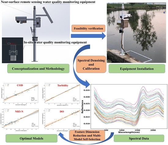
In this study, a set of automatic near-surface water quality monitoring systems (Figure 1a,b) were built to realize the non-contact and high accuracy measurement of water quality parameters. It is mainly composed of visible sphere machines (Hangzhou Hikvision Digital Technology Co., Ltd., Hangzhou, China), radar flowmeters (Chongqing Hayden Technology Co., Ltd., Chongqing, China), small weather stations (Shandong Renke Measurement and Control Co., Ltd., Jinan, China), self-developed hyperspectral imagers based on linear variable filters (LVF), and rotary calibration devices. The system already has the ability to collect data automatically, the stability test of hardware has passed, and a set of supporting software written by C# has been developed. Visible sphere machines are mainly used to display real-time pictures of the environment near the device and also to reflect the floating objects on the water surface through color images of the water surface. Radar flowmeters can monitor the water level and flow of current water bodies. Small weather stations can obtain some meteorological data, such as temperature and humidity, rainfall, light, wind speed, and wind direction.

The hyperspectral imager (Figure 1c) is the core equipment developed by our laboratory team. The rotary calibration device is used in combination with the hyperspectral imager. When the hyperspectral imager works, the calibration plate (30% spectral reflectance) made of Teflon is transferred to the horizontal orientation through the rotary motor, and at the other time, the calibration plate shrinks to the holding box. This measure is to prevent the calibration board from being polluted, reduce the maintenance cycle, and realize the automatic calibration of data without being on duty. The hyperspectral imager is specifically composed of a front telescope unit, a coupled splitter unit, and a data processing unit. The operating principle (Figure 2a) adopted is the reflected light of the target of incident to the front telescope unit, which then enters the field aperture through the beam compression of the telescope group, passes through the imaging lens group, and finally forms an image on the detector surface. The surface of the detector is windowed and coated, and a pixel-level modulation linear gradient filter module is integrated. After LVF splitting, monochromatic light with different wavelengths occurs at different positions, and the target spectral images with different wavelengths are obtained by the detector. The front telescope system and the coupled splitter unit are distributed along the optical axis. The system has passed the comparison test (Figure 2c) with the ASD spectrometer (FieldSpec4 Hi-Res spectroradiometer, Analytical Spectra Devices, Inc., Boulder, CO, USA) and is feasible in specific application scenarios. The technical indicators (

Table 1. Technical indicators for hyperspectral imager.

Indicator	Parameter
Spectral range	430 nm~850 nm
Spatial resolution	≤0.3 mrad
Spectral resolution	≤5 nm
MTF	≥0.5
F/#	≤5
FOV	24.84°
Integration	Usually 6000 $\mathsf{\mu }\mathrm{s}$
Weight/kg	<1.5 kg

) of the hyperspectral imager can meet the requirements of specific scenario applications. The technical scheme ensures the requirements of light and a small-scale system, the synchronous acquisition of multi-dimensional spectral information, efficient information reconstruction and so on.

The system is installed by placing a visible sphere machine, a radar flowmeter, and a hyperspectral imager in a custom storage box fixed on the horizontal pole and a small weather station on top of the vertical pole. The rotary calibration device is placed in the middle of the vertical pole, 70 cm from the height of the horizontal pole so that the hyperspectral imager does not lose focus and the calibration plate occupies an appropriate area of view. The height of the pole can be set to 2–5 m, fixed on the shore (in an open position, where water depth is not visible to the naked eye), and where the pole is facing the water. It is best to install the pole in the North–South direction so that it can avoid the influence of the pole’s own shadow and ensure the equipment works uninterrupted during the day. It is important to note that the system needs to be used with in situ water quality monitoring equipment (Figure 1d) in the early stage. In this aspect, the lab team has performed a good job, and it has been applied in water plants, urban inland rivers, and other scenarios. Self-developed in situ water quality monitoring equipment has been updated for several generations; MWIS-3000 is the latest model, which has been laid out in the Poyang Lake, Xiangxi River, and Dasha River in Shenzhen. A large amount of water quality data can be obtained, including Chl-a, DO, COD, turbidity, NH3-N, NO3-N, pH, temperature, and so on. Using the software developed by our team based on C#, various water quality parameters can be obtained in seconds, and cloud storage and remote transmission can be achieved. The in situ water quality monitoring equipment is immersed in the water below the pole body and works synchronously with the pole equipment to obtain the measured values of the water quality parameters, which will be used as labels to assist in the evaluation and selection of models. All the equipment that can be controlled is connected to the industrial control computer (Figure 2b) in the control box through a USB or COM port, which enables data management and evaluation decisions in the data cloud management platform. The power supply mode can be either mains or solar. The set of equipment in this study is expected to be used in lakes, rivers, reservoirs, ponds, and other scenarios. Because of its high spatial resolution, it can be used in large and small water bodies. In addition, a high temporal resolution enables the high-frequency continuous acquisition of data.

2.2. Study Area

The study area (Figure 3) was selected in a large fish pond (400 square meters in area and 2 m in water depth) in the southeast of Xi’an, Shaanxi Province, China. The water source of the fish pond comes from the Yuhe river, which originates from Dayu on the northern slope of the Qinling Mountains. It is the most famous river in Xi’an, with a total length of 64.2 km, a drainage area of 687 square kilometers and an average runoff of 210.5 million cubic meters. Water quality is the key in aquaculture [20]. The fish pond is rich in biodiversity. Due to temperature changes, biological respiration and photosynthesis, the water quality of the fish pond has changed greatly, so it was very suitable to take this place as the research area.

2.3. Field Data Collection

At present, the method to obtain the measured values of water quality parameters in most studies is to put water into bottles and take it back to the laboratory or hand it over to professional institutions for artificial chemical measurement [9,10,11]. The feasibility of this method needs to be verified. The first, is that the water quality parameters in the bottle undergo subtle changes due to the activities of microorganisms [21]. The second is the preservation of the water samples. Strictly speaking, they should be stored at low temperatures in an environment with a pH < 2 [22]. However, due to the complex environmental conditions at the sampling point, such strict preservation conditions are often not achieved. Third, this artificial chemical method is easy to cause secondary pollution, which is time-consuming, laborious, and makes it easy to introduce artificial errors [3], such as the dichromate method for measuring COD (HJ 828-2017), iodometric method for measuring dissolved oxygen (GB 7489-87), and Nessler reagent spectrophotometry for measuring ammonia nitrogen (HJ 535-2009), etc. The corresponding label value of the spectral information obtained by remote sensing must be time-dependent. Manual samplings and chemical measurements may bring great deviation to the measured value results, which is not conducive to the establishment of the subsequent models.

Since the concentration of Chl-a in the fishpond has reached more than 400 $\mathsf{\mu }\mathrm{g}/\mathrm{L}$, it exceeds the range of most existing sensors. Both TN and TP parameters [23] have poor sensor accuracy and time continuity (with a time interval greater than 40 min). Turbidity is a representative parameter because it has a strong correlation with parameters such as transparency, total suspended matter, and chroma [24]. In this study, four water quality parameters (COD, DO, turbidity, and NH3-N) were selected to study, taking into account the water quality of the fishpond and the use of existing sensors. Using the in situ water quality monitoring equipment (

Table 2. Detailed parameters of four underwater sensors.

Variable	Method	Detection Limit (Lower-Upper Limit)	Accuracy	Repeatability	Resolution Ratio
COD	Ultraviolet absorption method	0–1000 mg/L	±5%	±2%	0.01 mg/L
DO	Fluorescence quenching method	0–20 mg/L	±3%	±3%	0.01 mg/L
Turbidity	Combined infrared absorption and scattering method	0.01–4000 NTU	±2%	±2%	0.1 NTU
NH3-N	Ion selective electrode method (pH reference, potassium ion compensation)	0.1–1000 mg/L	±5%	±5%	0.01 mg/L

) developed by our laboratory, data (

Table 3. Summary statistics of the main variables of data set (88 groups).

Variable	Unit	Mean	Median	Minimum	Maximum	SD
COD	mg/L	18.71	18.56	13.92	22.51	2.18
DO	mg/L	11.76	13.30	2.21	19.90	3.99
Turbidity	NTU	16.91	12.95	6.84	39.20	8.64
NH3-N	mg/L	0.53	0.42	0.13	1.71	0.38

) were collected continuously from 25 April 2022 to 6 June 2022 to obtain a 10 s interval of data for the four water quality parameters. In addition, in order to ensure the authenticity of the measured data, the in situ underwater probe maintains a frequency of manual maintenance once a week, and the probe also has its own brush to achieve a certain degree of self-cleaning. At the same time, the hyperspectral imager is working (2–3 times a day), taking 88 valid images (Figure 4) during the study period, and contains the spectral information for both the calibration plate and the measured water body.

2.4. Data Preprocessing

2.4.1. Outlier Removal

The measured values of the four water quality parameters obtained by the in situ water quality monitoring equipment rarely deviated seriously but considering that few outliers may have a serious impact on the model, a detection method was needed to remove the outliers. Considering the cause of the outliers, it may be that there are large particles near the optical probe (COD, turbidity, and DO probes are based on optical principles) and ion selective electrodes (NH3-N), blocking the optical window and selective transmission membrane. Although the filter device was installed, it was found that large algae and even fish fry could still appear in the filter screen during maintenance. Due to the eutrophication of the fishpond water body and intense biological activities, algae spores and fish eggs could also still pass through the fine pores of the filter screen due to their small volume.

This study chose to use the local outlier factor (LOF) algorithm to detect outliers [25]. LOF is a classical algorithm based on density. Previous outlier detection methods are mostly based on statistical methods or clustering algorithms. The LOF algorithm is widely used by researchers because of its simplicity and ease of use, without considering data distribution and other advantages. The LOF algorithm has a basic assumption: that the density around the non-outliers is similar to that around its neighborhood, while the density around the outliers is significantly different from that around its neighborhood.

2.4.2. Spectral Denoising

In this study, the height of the pole equipment was low, and the field of vision was small. It can be assumed that the water quality parameters within the field of vision were uniform in a short time. The spectral image taken by the hyperspectral imager, whose design was based on LVF, contained the spectral information (430~850 nm) of the target, and the wavelength of the image band gradually increased from left to right. Under the assumption that the reflectance of the target was uniform, the spectral curve of the target could be obtained through a two-dimensional image. The advantage of this method was to reduce the temporal and spatial complexity caused by the stitching of hyperspectral images into data cubes and increase the possibility of real-time processing.

In order to obtain a true and accurate spectral curve, this study proposes a spectral denoising method (Figure 5) that can remove the effects of debris and ripples on the water surface. In view of the low reflectivity of the water to sunlight and sky light and the high reflectivity of the debris and ripples floating on the water compared with the water itself, when extracting the spectral curve according to the row direction, the water surface noise showed obvious peaks. When the water surface noise had an impact, the abnormal signal value could be replaced by other normal signal values in the same column. Due to the uncertainty of the area of water surface noise, it is best to take the first quartile or the first decile of all signal values of the same wavelength band as the signal value of the current wavelength.

In addition, sometimes, due to the signal-to-noise ratio of the instrument does not reach the optimal working state, or the combined effect of dark current and other interference factors, there is a certain amount of noise in the spectral reflectance of different bands, resulting in the serrated reflectance of adjacent bands. In order to improve the accuracy of information extraction, filtering smoothing is required. The Savitzky-Golay (S-G) filtering method used in this study is a filtering method based on local polynomial least squares fitting in time domain [26]. The most important feature is that the shape and width of the signal can be kept unchanged while the noise is filtered. Its algorithm idea is to achieve noise suppression by moving smoothly. The S g filtering method in this study used the window length of 17, the polynomial order of 3, and the mode of ‘nearest’.

2.4.3. Calibration

In order to obtain a real remote sensing reflectance, calibration is an essential step. Calibration refers to the process of converting the signal value (generally referred to as the DN value) detected by the hyperspectral imager into reflectance. According to Mobley’s [27] method, the influence of sky light needs to be considered. In different time periods (from 8:00 a.m. to 6:00 p.m. on different days) and during different weather conditions (cloudy or cloudless, sunny, or overcast), 18 sets of data were collected in the fishpond experimental site with reference to Mobley’s method (a viewing direction of 40 degrees from the nadir and 135 degrees from the sun). However, after the author’s repeated verification and analysis, the influence of sky light only accounted for less than 5% (Figure 6). The reason for this may be that the small inland water body is always calm, which meets the optimal collection conditions. Therefore, it is acceptable to ignore the sky light [28]. In addition, considering that the pole equipment can not rotate the lens angle and direction randomly according to the solar altitude angle, unlike the manual experiment, the remote sensing reflectance is characterized by the ratio of the total vertical radiance ($W·m^{-2}·n{m}^{-1}·s{r}^{-1}$) and the total incident irradiance on the water surface ($W·m^{-2}·n{m}^{-1}$). The formula is as follows:

$$R_{rs}=L_v/E_d\left(0^{+}\right)$$

(1)

$$E_d\left(0^{+}\right)=L_p\times \pi /{\rho }_p$$

(2)

where $R_{rs}$ is remote sensing reflectance, $L_v$ is the total vertical radiance from water, $E_d\left(0^{+}\right)$ is the total incident irradiance on the water surface (multiple average calculation), $L_p$ is the radiance of the calibration plate, ${\rho }_p$ is the reflectance of the calibration plate, and the standard gray plate with a reflectance of 10–30% after calibration is selected through the calibration plate.

After spectral denoising and calibration, the reflectance spectral curve (Figure 7) of the water body showed good stability. In the blue band between 490 nm and 510 nm, it is clear that chlorophyll-a and carotenoids strongly absorbed the blue and purple light, while organic debris, inorganic suspended matter and yellow substances also had a certain absorption effect in this range, which made the reflection of the water body in this wavelength range relatively low, and the first absorption valley appear. The reflectance gradually increased in the range of 510 nm~570 nm, and the range of 560 nm~580 nm is the first reflection peak of the spectral curve. At the same time, it reaches a maximum peak at about 570 nm, which is one of the remarkable characteristics of turbid water and is also called the first reflection peak of the sediment. Since the reflection peak at 570 nm wavelength is caused by the weak absorption of chlorophyll-a and the co-scattering of cells and a large number of suspended matter in the water, a 570 nm wavelength can also be used as one of the important indicators for the quantitative retrieval of chlorophyll-a. The two obvious absorption valleys near 670 nm and 760 nm are generally considered to have been caused by the strong absorption of the cyanobacteria protein in the red band, which was also considered to be one of the signs of chlorophyll-a retrieval. The 720 nm reflection peak is usually considered to be caused by the fluorescence effect of phytoplankton after absorbing light. This is one of the most significant bases for judging whether there is chlorophyll-a in the water body. However, the position of the peak here is generally unstable, and a “red shift” will occur with an increase in chlorophyll-a concentration [29]; The reflectance decreases sharply after 720 nm until the change of the spectral curve at 760 nm shows a flat state. The third reflection peak near 820 nm is called the second reflection peak of the sediment, which is an important indication of the existence of suspended matter in the water. It is formed by backscattering with a continuous increase in sediment concentration. When the wavelength is greater than 820 nm, the reflectance begins to decline due to the absorption of water in the near-infrared band [30,31,32].

2.4.4. Feature Dimension Reduction

Hyperspectral data contains a lot of redundant information. If it is input into the model without dimension reduction, it will increase the amount of the calculation and affect the accuracy of the regression prediction. This study presents a robust feature dimension reduction method based on principal component analysis (PCA), Pearson correlation analysis (PCA*), and the random forest regression (RFR) algorithm. PCA is an orthogonal linear transform based on information quantity. The transformed spectral information is mainly concentrated in the first few principal components, and the components with a small amount of information are discarded in the transform domain [33]. The Pearson correlation coefficient reflects the degree of linear correlation between the two variables. The greater the absolute value of $r$, the stronger the correlation [34]. Random forest regression records the importance of each feature during the algorithm process [35,36]. In order to make full use of the above algorithms, the first unsupervised principal component extraction was carried out for all the features, and the principal components of the top three were selected as the feature dimension. Secondly, Pearson correlation analysis was performed on the spectral data and each measured water quality parameter value in the training set, and PCA dimension reduction was performed on several bands with the largest absolute Pearson correlation coefficient. The first three principal components in the order were used as the feature dimension. Then, the spectral data and each measured water quality parameter value in the training set were used for random forest regression. The first bands sorted by feature importance were selected for PCA dimension reduction, and the first three principal components were used as the feature dimension. Finally, the nine feature dimensions of the preceding steps were combined and input into the model. The feature dimension reduction algorithm used in this study deleted redundant information while maximizing useful spectral information. Combining supervised learning with unsupervised learning and making full use of the prior information, retrieval accuracy was improved by inputting dimension-reduced features into the model. In the process of feature dimension reduction, the relationship between the four water quality parameters and related bands was found (

Table 4. Several bands most related to four water quality parameters (sorted in descending order of correlation).

Variable	Related Band
COD	640 nm, 580 nm, 720 nm
Turbidity	720 nm, 810 nm, 580 nm, 520 nm
NH3-N	720 nm, 750 nm, 630 nm
DO	720 nm, 540 nm, 810 nm

). The implementation of PCA and RFR was based on Python 3.6 and scikit-learn libraries. The formula for the Pearson correlation coefficient is as follows:

$$r=\frac{{\sum }_{i=1}^n\left(X_i-\overline{X}\right)\left(Y_i-\overline{Y}\right)}{\sqrt{{\sum }_{i=1}^n{\left(X_i-\overline{X}\right)}^2}\sqrt{{\sum }_{i=1}^n{\left(Y_i-\overline{Y}\right)}^2}}$$

(3)

where $\overline{X}$ is the mean of $X$, and $\overline{Y}$ is the mean of $Y$.

2.5. Machine Learning Models

This study applied fourteen machine learning algorithms, including linear regression (LR), ridge regression (RR), least absolute shrinkage and selection operator regression (LASSO), elastic net regression (ENR), k-nearest neighbor regression (KNN), Gaussian process regression (GPR), decision tree regression (DTR), support vector regression (SVR), multilayer perceptron regression (MLP), adaptive boosting regression (ABR), gradient boosting regression (GBR), bootstrap aggregating regression (Bagging), random forest regression (RFR), and extreme tree regression (ETR) to build the retrieval model, and finally selected the most suitable one to estimate the concentration of the four water quality parameters(COD, DO, turbidity, and NH3-N).

All the machine learning models used in this study are supervised models, which are divided into single and ensemble learning models. The single models include the linear model, KNN, GPR, DTR, SVR, and MLP. Linear models include LR, LASSO, RR, and ENR. The ensemble learning models include the Boosting and Bagging models, where the Boosting models contain GBR and ABR, and Bagging models contain RFR and ETR.

LR, also known as partial least squares regression, is a regression analysis that can model the relationship between one or more independent and dependent variables. The principle of the algorithm is to use the partial least squares method to minimize the square error [37]. RR is a linear least square method with L2 regularization. It is a biased estimation regression method specially used for linear data analysis. By giving up the unbiasedness of the least square method, the regression coefficient is obtained at the cost of losing part of the information and reducing the accuracy. Ridge regression is very useful when there is collinearity in the data set, and the regression coefficient obtained by LR is more practical and reliable. In addition, it can make the fluctuation range of the estimated parameters smaller and more stable [38]. Similar to RR, LASSO adds a penalty value to the absolute value of the regression coefficient [39]. The difference with RR is that it uses an absolute value instead of square value in the penalty part. ENR is a mixture of LASSO and RR. RR is a biased analysis of the cost function using the L2-norm (square term). LASSO uses the L1-norm (absolute value term) to conduct a biased analysis of the cost function. ENR combines the two, using both the square term and the absolute value term [40].

When calculating the predicted value of a data point using KNN, the model selects the k-nearest data points from the training data set and averages their label values, using the mean as the predicted value for the new data point [41]. GPR is a non-parametric model that uses a Gaussian process prior to the regression analysis of data. The GPR model assumes two parts, noise (regression residuals) and a Gaussian process prior, and its solution is based on Bayesian inference. Without restricting the form of the kernel function, GPR is theoretically a universal approximator for any continuous function in q compact space. In addition, the GPR provides a posteriori of predictions, which can be parsed when the likelihood is normally distributed. Therefore, GPR is a probability model with generality and resolvability [42]. An advantage of the DTR is that it does not require any transformation of the features if we are dealing with nonlinear data. A decision tree is grown by iteratively splitting its nodes until the leaves are pure or a topping criterion is satisfied [43]. SVR creates an interval zone on both sides of the linear function with a spacing of $ϵ$ (also known as tolerance bias, which is an empirical value set manually); no loss is calculated for the samples falling into the interval zone, that is, only support vectors will have an impact on its function model, and the optimized model is obtained by minimizing the total loss and maximizing the interval [44]. MLP is a network of fully connected layers with at least one hidden layer whose output is transformed by an activation function. The number of layers in a multilayer perception machine and the number of hidden cells in each hidden layer are hyperparameters [45].

ABR calculates and re-weights the weights of the learners based on their current performance and then selects the median weighted learner as a result by sorting the weights of the learners [46]. The basic idea of GBR is that multiple weak learners are generated serially, and the goal of each weak learner is to fit the negative gradient of the loss function of the previous accumulation model so that the cumulative model loss with the weak learner decreases in the direction of the negative gradient [47]. Bagging’s step is to first sample $T$ sample sets with $m$ samples, then train a learner based on each sample set before finally combining the learners and using the mean method for regression tasks [48].

RFR [35] is an ensemble technique that combines multiple decision trees. A random forest usually has a better generalization performance than an individual tree due to randomness, which helps to decrease the model’s variance. Other advantages of random forests are that they are less sensitive to outliers in the dataset and do not require much parameter tuning. The only parameter in random forests that we typically need to experiment with is the number of trees in the ensemble. The only difference is that we use the MSE criterion to grow the individual decision trees, and the predicted target variable is calculated as the average prediction over all the decision trees. ETR and RFR are very similar, but there are two main differences: (1) Each tree in ETR uses all the training samples- that is, the sample set of each tree is the same. (2) RFR selects the optimal bifurcation feature in the feature subset, while ETR selects the bifurcation feature directly and randomly [4,49].

In this study, the above fourteen machine learning regression algorithms are not described in detail; the algorithms were implemented using python 3.6 and scikit learn libraries. The specific information of the training hardware platform is as follows: the CPU is intel core i7 10TH GEN, the graphics card is NVIDIA GeForce RTX 3060 12G, and the memory size is 16G. The operating system is Ubuntu Desktop 20.04 LTS.

2.6. Accuracy Assessment

Mean absolute error (MAE) is the average of absolute errors, which better reflects the actual situation of the prediction error. The root mean square error (RMSE) is the root of the mean square error, which represents the sample standard deviation between the estimated and measured values. The coefficient of determination ($R^2$) reflects the accuracy of the data fitted by the model. The closer the value is to 1, the stronger the explanatory power of the equation variables is to y, and the better the model fits the data. For the mean absolute percentage error (MAPE), theoretically, the smaller the MAPE is, the better the prediction model fits. Accuracy (Acc) refers to the proportion of samples whose relative error (RE) is less than a certain threshold value in the total sample [50,51]. The formulas for the above indicators are as follows:

$$MAE=\frac{1}{n}{\sum }_{i=1}^n\left|y_i-{\widehat{y}}_i\right|$$

(4)

$$RMSE=\sqrt{\frac{1}{n}{\sum }_{i=1}^n{\left(y_i-{\widehat{y}}_i\right)}^2}$$

(5)

$$MAPE=\frac{100\%}{n}{\sum }_{i=1}^n\left|\frac{y_i-{\widehat{y}}_i}{y_i}\right|$$

(6)

$$R^2=1-\frac{{\sum }_{i=1}^n{\left(y_i-{\widehat{y}}_i\right)}^2}{{\sum }_{i=1}^n{\left(y_i-\overline{y}\right)}^2}$$

(7)

$$RE=\frac{\left|y_i-{\widehat{y}}_i\right|}{y_i}\times 100\%$$

(8)

$$Acc=\frac{N_a}{N}\times 100\%$$

(9)

where $y_i$ is the measured value, ${\widehat{y}}_i$ is the estimated value, $\overline{y}$ is the measured mean value, N is the sample capacity, and $N_a$ is the number of estimated values of RE within a threshold value. In this study, MAE, RMSE, MAPE, $R^2,$ and Acc are used to comprehensively evaluate the retrieval model.

3. Results

All the water quality data (including the seven parameters: Chl-a, COD, Conductivity, DO, pH, NH3-N, and turbidity) obtained in this study were analyzed for correlation, and a heatmap (Figure 8) was generated to visually represent the positive and negative correlation between variables. It was found that Chl-a had a high positive correlation with DO and a high negative correlation with NH3-N. DO was highly negatively correlated with NH3-N. COD was highly positively correlated with turbidity. This is because as algae reproduce, photosynthesis intensifies, and a large amount of oxygen is generated, which leads to an increase in DO. However, an increase in NH3-N inhibited the growth of algae. In addition, organic matter and reducing inorganic matter in water are the main factors affecting COD. Sediment and suspended matter in the water will still absorb organic matter, so COD will still increase with the increase in turbidity [14,52,53,54,55].

After the outliers of 88 groups of the original data were removed based on the LOF algorithm (configuration = 0.1), 79 groups of “clean” data were left. Then, the dataset was divided into 60 sets of training data and 19 sets of test data according to a 3:1 scale. The results of the feature selection for each water quality parameter by the feature dimension reduction step will be discussed later. Machine learning algorithms were implemented based on the sklearn library. RR, LR, GBR, KNN, DTR, ETR, ABR, and bagging used default parameters. The lasso and ETR’s alpha was set to 0.001. The SVR selected the RBF kernel, and C was set to 500. The RFR’s n_estimator was set to 200. GPR selected the constant kernel and RBF kernel, while the n_restarts_optimizer was set to 10, and the alpha was set to 0.01. The MLP’s hidden_layer_size was set to (8, 4), activation was set to ‘logistic’, the solver was set to ‘lbfgs’, the alpha was set to 0.01, and the max_iter was set to 200.

In this study, we chose scatter-line diagrams (Figure 9) to evaluate the accuracy of the model on the test dataset. In the scatter-line diagram, the blue points represent the measured values, and the curves of different colors represent the regression prediction results of the 14 different models. It was found that most models fitted accurately. Next, for each water quality parameter, the first four groups of optimal models are selected for display.

3.1. COD

After supervised feature dimension reduction in the COD training dataset, it was found that the selected spectral feature bands were mainly concentrated at 580, 640, and 720 nm. COD concentration significantly affected the spectral response at the yellow-green light junction and the red light, so the three bands above could be used for the effective retrieval of COD concentration. After comparing and evaluating several models (

Table 5. Performance of fourteen models on COD training dataset and test dataset.

COD	Training Dataset					Test Dataset
	${\mathit{R}}^{\mathbf{2}}$	RMSE (mg/L)	MAE (mg/L)	MAPE	Acc	${\mathit{R}}^{\mathbf{2}}$	RMSE (mg/L)	MAE (mg/L)	MAPE	Acc
LR	0.65	1.23	1.05	5.70%	85.71%	0.25	1.81	1.45	7.60%	77.78%
RR	0.14	1.93	1.6	8.58%	62.50%	0.08	2.02	1.71	9%	55.56%
LASSO	0.61	1.31	1.16	6.31%	83.93%	0.42	1.58	1.37	7.20%	83.33%
ENR	0.35	1.69	1.41	7.63%	67.86%	0.23	1.83	1.58	8.33%	66.67%
KNN	0.65	1.23	1.02	5.47%	89.29%	0.72	1.1	0.89	4.48%	94.44%
GPR	0.55	1.4	1.19	6.31%	82.14%	0.47	1.52	1.24	6.37%	77.78%
DTR	1	0	0	0	100%	0.83	0.87	0.53	2.89%	94.44%
SVR	0.89	0.71	0.41	2.28%	94.64%	0.49	1.49	1.09	5.57%	72.22%
MLP	0.82	0.89	0.7	3.85%	94.64%	0.68	1.18	0.88	4.47%	94.44%
ABR	0.97	0.38	0.31	1.74%	100%	0.87	0.76	0.49	2.65%	94.44%
GBR	1	0.04	0.03	0.18%	100%	0.86	0.79	0.53	2.85%	94.44%
Bagging	0.95	0.45	0.29	1.65%	98.21%	0.92	0.6	0.45	2.41%	100%
RFR	0.95	0.44	0.33	1.83%	100%	0.88	0.72	0.51	2.78%	94.44%
ETR	1	0	0	0	100%	0.63	1.27	0.88	4.65%	77.78%

, Figure 10) by comprehensive indexes, Bagging, RFR, ABR, and GBR were found to have the best fitting effect to COD and $R^2$ in the test dataset, which can reach 0.92, 0.88, 0.87, and 0.86, respectively. MAPE can reach a minimum of 2.41%, and accuracy can reach 100% with a tolerance of 10% relative error.

3.2. Turbidity

After feature dimension reduction in the turbidity training dataset, it was found that the selected spectral feature bands were mainly concentrated at 520, 580, 720, and 810 nm. Turbidity concentration significantly affected the spectral response at green, yellow, red, and near-infrared light, so the four bands above could be used for the effective retrieval of turbidity concentration. After comparing and evaluating several models (

Table 6. Performance of fourteen models on turbidity training dataset and test dataset.

Tur	Training Dataset					Test Dataset
	${\mathit{R}}^{\mathbf{2}}$	RMSE (mg/L)	MAE (mg/L)	MAPE	Acc	${\mathit{R}}^{\mathbf{2}}$	RMSE (mg/L)	MAE (mg/L)	MAPE	Acc
LR	0.65	4.61	3.59	26.98%	64.29%	0.6	6.85	5.6	24.59%	66.67%
RR	0.6	4.98	3.85	27.82%	62.50%	0.57	7.06	5.73	23.61%	66.67%
LASSO	0.63	4.79	3.73	27.27%	64.29%	0.56	7.13	5.9	25.25%	61.11%
ENR	0.62	4.8	3.73	27.13%	64.29%	0.57	7.07	5.82	24.54%	66.67%
KNN	0.62	4.86	2.89	17.60%	76.79%	0.4	8.37	5.84	20.80%	66.67%
GPR	0.95	1.77	1.26	8.59%	96.43%	0.78	5.09	3.9	17.88%	88.89%
DTR	1	0	0	0	100%	0.61	6.78	3.28	12.63%	88.89%
SVR	0.98	1	0.32	1.88%	100%	0.65	6.4	4.29	18.03%	77.78%
MLP	0.99	0.68	0.46	3.53%	100%	0.84	4.28	2.62	11.23%	94.44%
ABR	0.9	0.89	0.71	5.81%	100%	0.87	3.91	2.25	10.80%	88.89%
GBR	1	0.15	0.12	0.97%	100%	0.78	5.04	2.83	11.94%	88.89%
Bagging	0.92	2.19	0.99	7.16%	94.64%	0.93	2.77	2.13	9.70%	100%
RFR	0.95	1.82	1.01	6.73%	94.64%	0.89	3.58	2.7	11.35%	100%
ETR	1	0	0	0	100%	0.98	1.71	1.37	8.27%	94.44%

, Figure 11) by comprehensive indexes, ETR, Bagging, RFR, and ABR were found to have the best fitting effect for turbidity, and $R^2$ in the test dataset, which can reach 0.98, 0.93, 0.89, and 0.87, respectively. MAPE can reach a minimum of 8.27%.

3.3. NH3-N

After analysis, the NH3-N concentration significantly affected the spectral response of the red band (720 nm, 750 nm). After comparison and evaluation (

Table 7. Performance of fourteen models on NH3-N training dataset and test dataset.

NH3-N	Training Dataset					Test Dataset
	${\mathit{R}}^{\mathbf{2}}$	RMSE (mg/L)	MAE (mg/L)	MAPE	Acc	${\mathit{R}}^{\mathbf{2}}$	RMSE (mg/L)	MAE (mg/L)	MAPE	Acc
LR	0.6	0.19	0.15	43.39%	41.67%	0.63	0.31	0.26	49.82%	42.11%
RR	0.58	0.19	0.15	42.95%	41.67%	0.66	0.3	0.25	46.56%	42.11%
LASSO	0.58	0.19	0.15	42.56%	41.67%	0.65	0.3	0.25	46.04%	42.11%
ENR	0.58	0.19	0.15	42.61%	41.67%	0.66	0.3	0.25	46.13%	42.11%
KNN	0.79	0.14	0.1	27.87%	75%	0.7	0.28	0.22	29.14%	47.37%
GPR	0.9	0.09	0.07	21.68%	81.67%	0.85	0.19	0.15	24.57%	57.89%
DTR	1	0	0	0	100%	0.79	0.23	0.15	25.37%	63.16%
SVR	0.92	0.09	0.08	24.50%	70%	0.86	0.19	0.14	27.34%	57.89%
MLP	0.92	0.08	0.06	20.18%	83.33%	0.78	0.24	0.17	28.39%	52.63%
ABR	0.93	0.08	0.07	22.93%	71.67%	0.95	0.12	0.1	22.25%	78.95%
GBR	1	0.01	0.01	2.82%	100%	0.85	0.2	0.14	22.50%	68.42%
Bagging	0.92	0.09	0.05	14.28%	90%	0.81	0.22	0.18	23.92%	63.16%
RFR	0.95	0.07	0.05	14.22%	88.33%	0.88	0.17	0.14	22.41%	68.42%
ETR	1	0	0	0	100%	0.72	0.27	0.18	30.82%	47.37%

, Figure 12), ABR, RFR, SVR, and GPR were found to fit NH3-N best, where $R^2$ can reach 0.95, 0.88, 0.86, and 0.85, respectively, in the test set. MAPE can reach a minimum of 22.25%.

3.4. DO

Through the Pearson correlation analysis, there was a strong linear relationship between the DO concentration and spectral response at the red light (720 nm); therefore, most models, including linear models, had good results ($R^2$> 0.8). In addition, the spectral response at the green and near-infrared light is also related to the DO concentration. After comparison and evaluation (

Table 8. Performance of fourteen models on DO training dataset and test dataset.

DO	Training Dataset					Test Dataset
	${\mathit{R}}^{\mathbf{2}}$	RMSE (mg/L)	MAE (mg/L)	MAPE	Acc	${\mathit{R}}^{\mathbf{2}}$	RMSE (mg/L)	MAE (mg/L)	MAPE	Acc
LR	0.86	1.26	1.02	9.98%	96.67%	0.84	1.52	1.27	13.69%	89.47%
RR	0.85	1.3	1.03	9.97%	96.67%	0.83	1.59	1.34	13.97%	89.47%
LASSO	0.85	1.27	1.01	9.95%	95.00%	0.84	1.53	1.28	13.66%	89.47%
ENR	0.85	1.27	1.02	9.96%	96.67%	0.84	1.54	1.28	13.51%	94.74%
KNN	0.91	1	0.79	8.64%	96.67%	0.68	2.18	1.8	21.39%	63.16%
GPR	0.94	0.81	0.66	6.42%	98.33%	0.88	1.34	1.08	12.08%	94.74%
DTR	1	0	0	0	100%	0.83	1.57	1.2	12.83%	94.74%
SVR	1	0.11	0.1	0.97%	100%	0.68	2.17	1.71	19.15%	73.68%
MLP	1	0.23	0.16	1.23%	100%	0.91	1.16	0.99	10.59%	94.74%
ABR	0.96	0.64	0.53	4.37%	100%	0.86	1.42	1.2	13.86%	89.47%
GBR	1	0.08	0.06	0.56%	100%	0.85	1.47	1.17	15.34%	84.21%
Bagging	0.98	0.6	0.41	4.95%	96.67%	0.78	1.8	1.49	19.37%	73.68%
RFR	0.98	0.46	0.36	3.93%	98.33%	0.82	1.62	1.33	16.95%	73.68%
ETR	1	0	0	0	100%	0.82	1.61	1.21	14.27%	84.21%

, Figure 13), MLP, GPR, ABR, and GBR were found to fit DO best, where $R^2$ can reach 0.91, 0.88, 0.86, and 0.85, respectively, in the test dataset. MAPE can reach a minimum of 10.59%.

4. Discussion

4.1. Analysis of Experimental Results

In this study, the near-surface water quality monitoring equipment achieved excellent results through the Bagging for COD ($R^2$ = 0.92, RMSE = 0.6 mg/L, MAE = 0.45 mg/L, MAPE = 2.41%, Acc = 100%) ETR for Turbidity ($R^2$ = 0.98, RMSE = 1.71 mg/L, MAE = 1.37 mg/L, MAPE = 8.27%, Acc = 94.44%), ABR for NH3-N ($R^2$ = 0.95, RMSE = 0.12 mg/L, MAE = 0.1 mg/L, MAPE = 22.25%, Acc = 78.95%), and MLP for DO ($R^2$ = 0.91, RMSE = 1.16 mg/L, MAE = 0.99 mg/L, MAPE = 10.59%, Acc = 94.74%). In the process of feature dimension reduction, the characteristic bands for the four water quality parameters were found. The red and yellow-green light bands in the reflection spectrum are very important for water quality retrieval. This will provide a way to use empirical wavelengths to retrieve water quality parameters. The spectrometer a with narrow band range (such as the mosaic type) can be customized to 500–600 nm and 630 nm–760 nm wavelengths for water quality monitoring. In addition, in the selection of an algorithm model, the ensemble learning model performance is outstanding ($R^2$ > 0.8). This is because ensemble learning combines multiple base learners and is integrated into a strong learner with high robustness. The algorithm based on integrated learning has achieved the best results in the NETFLIX movie recommendation contest, KDD, and ICDM data mining contest in the United States. This study also shows the efficiency of ensemble learning in water quality parameter predictions.

4.2. Limitations and Future Optimization

First of all, although the system can image, its scope is limited, and it is essentially a point source type. Secondly, the optical complexity of turbulent waters may bring great uncertainty to the acquisition of spectral curves, such as the extremely fast velocity of water on the mainstream of the Yangtze River, accompanied by vortices. Finally, the difference of water bodies brings difficulties to the migration of models. Water quality parameters in different waters have different data ranges. For example, the chlorophyll concentration in many rivers is very low (<10 $\mathsf{\mu }\mathrm{g}/\mathrm{L}$), while the chlorophyll concentration in some lakes and reservoirs is very high (>100 $\mathsf{\mu }\mathrm{g}/\mathrm{L}$).

In the future, more deep learning models need to be explored. The recursive neural network [56], convolution neural network [57], capsule neural network [58] and other newer machine learning algorithms are good choices. The current four-parameter models for water quality have a certain prediction range, which is determined by the upper and lower limits of the concentration of the training set label itself. In view of the complexity of water components and the diversity of water types, each water body must be modeled specifically. In addition, the precision rotating platform can be used to carry self-developed hyperspectral imagers to increase the field of view, and the equipment can be erected in high terrain areas such as bridges, dams, etc., to complete the real-time monitoring of the application scenarios such as sewage outlets, where water blooms occur.

4.3. Potential Application

The water quality monitoring equipment and methods in this study have many advantages: (1) No station is needed, it is easy to set up, and in the long-term, it is maintenance-free. (2) Through in situ non-contact measurements, there is no danger of secondary pollution. (3) The radiation signal from the water is strong and does not need atmospheric correction. (4) It uses a fast measuring speed and many measuring indexes. (5) Remote models upgrade automatically, providing a more accurate measurement. (6) Water quality monitoring modes such as ship-borne, airborne and satellites can be used in collaboration to build a “space-air-ground integration” water quality monitoring mode [59,60]. In the future, it can be used in large, medium and small lakes, rivers, reservoirs and other places, especially in key sections, sensitive water sources and other places that need frequent monitoring. In addition, it can also be used for validation, such as in remote sensing data from satellites and unmanned aerial vehicles.

5. Conclusions

Based on the automatic near-surface water quality monitoring system and the in situ monitoring data, this study applies a series of preprocessing steps and fourteen machine learning algorithms, including LR, RR, LASSO, ENR, KNN, GPR, DTR, SVR, MLP, ABR, GBR, Bagging, RFR, and ETR, to build retrieval models for the COD, turbidity, NH3-N, and DO concentration in the fishpond. Additionally, the performance of fourteen algorithms is assessed by using $R^2$, MAE, RMSE, MAPE, and Acc. It is concluded that the spectral response in the red band is the key to the retrieval of the four water quality parameters. The results show that the determination coefficients of the four water quality parameters, namely COD, turbidity, NH3-N, and DO, are greater than 0.9. Moreover, ensemble learning models have higher robustness in the prediction of water quality parameters. This study proves the feasibility and high performance of the self-developed equipment and method. In the future, we will optimize the prediction algorithm and collect more data to improve the universality of the model.

References

1. Gupta, S.; Gupta, S.K. A critical review on water quality index tool: Genesis, evolution and future directions. Ecol. Inform. 2021, 63, 101299. [Google Scholar] [CrossRef]
2. Jaywant, S.A.; Arif, K.M. A Comprehensive Review of Microfluidic Water Quality Monitoring Sensors. Sensors 2019, 19, 4781. [Google Scholar] [CrossRef] [PubMed] [Green Version]
3. Nazeer, M.; Nichol, J.E. Development and application of a remote sensing-based Chlorophyll-a concentration prediction model for complex coastal waters of Hong Kong. J. Hydrol. 2016, 532, 80–89. [Google Scholar] [CrossRef]
4. Zhuang, Y.; Wen, W.; Ruan, S.; Zhuang, F.; Xia, B.; Li, S.; Liu, H.; Du, Y.; Zhang, L. Real-time measurement of total nitrogen for agricultural runoff based on multiparameter sensors and intelligent algorithms. Water Res. 2022, 210, 117992. [Google Scholar] [CrossRef] [PubMed]
5. Xiong, Y.; Ran, Y.; Zhao, S.; Zhao, H.; Tian, Q. Remotely assessing and monitoring coastal and inland water quality in China: Progress, challenges and outlook. Crit. Rev. Environ. Sci. Technol. 2019, 50, 1266–1302. [Google Scholar] [CrossRef]
6. Palmer, S.C.J.; Kutser, T.; Hunter, P.D. Remote sensing of inland waters: Challenges, progress and future directions. Remote Sens. Environ. 2015, 157, 1–8. [Google Scholar] [CrossRef] [Green Version]
7. Liu, H.; Yu, T.; Hu, B.; Hou, X.; Zhang, Z.; Liu, X.; Liu, J.; Wang, X.; Zhong, J.; Tan, Z.; et al. UAV-Borne Hyperspectral Imaging Remote Sensing System Based on Acousto-Optic Tunable Filter for Water Quality Monitoring. Remote Sens. 2021, 13, 4069. [Google Scholar] [CrossRef]
8. Schaeffer, B.A.; Schaeffer, K.G.; Keith, D.; Lunetta, R.S.; Conmy, R.; Gould, R.W. Barriers to adopting satellite remote sensing for water quality management. Int. J. Remote Sens. 2013, 34, 7534–7544. [Google Scholar] [CrossRef]
9. Sun, X.; Zhang, Y.; Shi, K.; Zhang, Y.; Li, N.; Wang, W.; Huang, X.; Qin, B. Monitoring water quality using proximal remote sensing technology. Sci. Total Environ. 2022, 803, 149805. [Google Scholar] [CrossRef]
10. Wang, W.; Shi, K.; Zhang, Y.; Li, N.; Sun, X.; Zhang, D.; Zhang, Y.; Qin, B.; Zhu, G. A ground-based remote sensing system for high-frequency and real-time monitoring of phytoplankton blooms. J. Hazard Mater. 2022, 439, 129623. [Google Scholar] [CrossRef]
11. Li, N.; Zhang, Y.L.; Shi, K.; Zhang, Y.B.; Sun, X.; Wang, W.J.; Huang, X. Monitoring water transparency, total suspended matter and the beam attenuation coefficient in inland water using innovative ground-based proximal sensing technology. J. Environ. Manag. 2022, 306, 114477. [Google Scholar] [CrossRef] [PubMed]
12. Boddula, V.; Ramaswamy, L.; Mishra, D. CyanoSense: A Wireless Remote Sensor System Using Raspberry-Pi and Arduino with Application to Algal Bloom. In Proceedings of the 2017 IEEE International Conference on AI & Mobile Services (AIMS), Honolulu, HI, USA, 25–30 June 2017; pp. 85–88. [Google Scholar]
13. Ouma, Y.O.; Waga, J.; Okech, M.; Lavisa, O.; Mbuthia, D. Estimation of Reservoir Bio-Optical Water Quality Parameters Using Smartphone Sensor Apps and Landsat ETM plus: Review and Comparative Experimental Results. J. Sens. 2018, 2018, 3490757. [Google Scholar] [CrossRef]
14. Gholizadeh, M.H.; Melesse, A.M.; Reddi, L. A Comprehensive Review on Water Quality Parameters Estimation Using Remote Sensing Techniques. Sensors 2016, 16, 1298. [Google Scholar] [CrossRef] [PubMed] [Green Version]
15. Guo, H.; Huang, J.J.; Chen, B.; Guo, X.; Singh, V.P. A machine learning-based strategy for estimating non-optically active water quality parameters using Sentinel-2 imagery. Int. J. Remote Sens. 2021, 42, 1841–1866. [Google Scholar] [CrossRef]
16. Niu, C.; Tan, K.; Jia, X.; Wang, X. Deep learning based regression for optically inactive inland water quality parameter estimation using airborne hyperspectral imagery. Environ. Pollut. 2021, 286, 117534. [Google Scholar] [CrossRef]
17. Dey, J.; Vijay, R. A critical and intensive review on assessment of water quality parameters through geospatial techniques. Environ. Sci. Pollut. Res. 2021, 28, 41612–41626. [Google Scholar] [CrossRef]
18. Huang, J.; Guo, H.; Chen, B.; Guo, X.; Singh, V. Retrieval of Non-Optically Active Parameters for Small Scale Urban Waterbodies by a Machine Learning-Based Strategy. Preprints 2020. [Google Scholar] [CrossRef] [Green Version]
19. Jiang, Q.; Xu, L.; Sun, S.; Wang, M.; Xiao, H. Retrieval model for total nitrogen concentration based on UAV hyper spectral remote sensing data and machine learning algorithms—A case study in the Miyun Reservoir, China. Ecol. Indic. 2021, 124, 107356. [Google Scholar]
20. Truong, T.M.; Phan, C.H.; Tran, H.V.; Duong, L.N.; Nguyen, L.V.; Ha, T.T. To Develop a Water Quality Monitoring System for Aquaculture Areas Based on Agent Model. In Fourth International Congress on Information and Communication Technology; Springer: Singapore, 2020; Volume 1027, pp. 47–58. [Google Scholar]
21. Kianpoor Kalkhajeh, Y.; Jabbarian Amiri, B.; Huang, B.; Henareh Khalyani, A.; Hu, W.; Gao, H.; Thompson, M.L. Methods for Sample Collection, Storage, and Analysis of Freshwater Phosphorus. Water 2019, 11, 1889. [Google Scholar] [CrossRef] [Green Version]
22. Sliwka-Kaszyska, M.; Kot-Wasik, A.; Namieśnik, J. Preservation and Storage of Water Samples. Crit. Rev. Environ. Sci. Technol. 2003, 33, 31–44. [Google Scholar] [CrossRef]
23. Lee, E.; Han, S.; Kim, H. Development of Software Sensors for Determining Total Phosphorus and Total Nitrogen in Waters. Int. J. Environ. Res. Public Health 2013, 10, 219–236. [Google Scholar] [CrossRef] [PubMed]
24. Petus, C.; Chust, G.; Gohin, F.; Doxaran, D.; Froidefond, J.-M.; Sagarminaga, Y. Estimating turbidity and total suspended matter in the Adour River plume (South Bay of Biscay) using MODIS 250-m imagery. Cont. Shelf Res. 2010, 30, 379–392. [Google Scholar] [CrossRef] [Green Version]
25. Breunig, M.; Kriegel, H.-P.; Ng, R.; Sander, J. LOF: Identifying Density-Based Local Outliers. In Proceedings of the 2000 ACM SIGMOD International Conference on Management of Data, Dallas, TX, USA, 15–18 May 2000; Volume 29, pp. 93–104. [Google Scholar]
26. Schafer, R.W. What Is a Savitzky-Golay Filter? [Lecture Notes]. IEEE Signal Process. Mag. 2011, 28, 111–117. [Google Scholar] [CrossRef]
27. Mobley, C. Estimation of the Remote-Sensing Reflectance from Above-Surface Measurements. Appl. Opt. 2000, 38, 7442–7455. [Google Scholar] [CrossRef]
28. Kutser, T.; Vahtmäe, E.; Paavel, B.; Kauer, T. Removing glint effects from field radiometry data measured in optically complex coastal and inland waters. Remote Sens. Environ. 2013, 133, 85–89. [Google Scholar] [CrossRef]
29. Gitelson, A. The peak near 700 nm on radiance spectra of algae and water: Relationships of its magnitude and position with chlorophyll concentration. Int. J. Remote Sens. 1992, 13, 3367–3373. [Google Scholar] [CrossRef]
30. Igamberdiev, R.M.; Grenzdoerffer, G.; Bill, R.; Schubert, H.; Bachmann, M.; Lennartz, B. Determination of chlorophyll content of small water bodies (kettle holes) using hyperspectral airborne data. Int. J. Appl. Earth Obs. Geoinf. 2011, 13, 912–921. [Google Scholar] [CrossRef]
31. Wang, F.; Zhou, B.; Liu, X.; Zhou, G.; Zhao, K. Remote-sensing inversion model of surface water suspended sediment concentration based on in situ measured spectrum in Hangzhou Bay, China. Environ. Earth Sci. 2012, 67, 1669–1677. [Google Scholar] [CrossRef]
32. Cheng, C.; Wei, Y.; Xu, J.; Yuan, Z. Remote sensing estimation of Chlorophyll a and suspended sediment concentration in turbid water based on spectral separation. Optik 2013, 124, 6815–6819. [Google Scholar] [CrossRef]
33. Jolliffe, I.T.; Cadima, J. Principal component analysis: A review and recent developments. Philos. Trans. A Math. Phys. Eng. Sci. 2016, 374, 20150202. [Google Scholar] [CrossRef] [Green Version]
34. Dai, X.L.; Zhu, P.Y.; Zhuang, Y.; Ding, J.B.; Wang, Y. Correlation study of tai lake conventional water quality. Oxid. Commun. 2015, 38, 1364–1372. [Google Scholar]
35. Breiman, L. Random forests. Mach. Learn. 2001, 45, 5–32. [Google Scholar] [CrossRef]
36. Huang, N.T.; Lu, G.B.; Xu, D.G. A Permutation Importance-Based Feature Selection Method for Short-Term Electricity Load Forecasting Using Random Forest. Energies 2016, 9, 767. [Google Scholar] [CrossRef] [Green Version]
37. Montgomery, D.C.; Peck, E.A.; Vining, G.G. Introduction to Linear Regression Analysis; NY John Wiley & Sons: New York, NY, USA, 1982. [Google Scholar]
38. Hoerl, A.E.; Kennard, R.W. Ridge regression: Biased estimation for nonorthogonal problems. Technometrics 2000, 42, 80–86. [Google Scholar] [CrossRef]
39. Osborne, M.R.; Turlach, P. On the LASSO and Its Dual. J. Comput. Graph. Stat. 2000, 9, 319–337. [Google Scholar]
40. Mol, C.D.; Vito, E.D.; Rosasco, L. Elastic-Net Regularization in Learning Theory. J. Complex. 2009, 25, 201–230. [Google Scholar] [CrossRef] [Green Version]
41. Burba, F.; Ferraty, F.; Vieu, P. Convergence of k nearest neighbor kernel estimator in nonparametric functional regression. Comptes Rendus Math. 2008, 346, 339–342. [Google Scholar] [CrossRef]
42. Rasmussen, C.E. Gaussian processes in machine learning. In Advanced Lectures on Machine Learning; Bousquet, O., VonLuxburg, U., Ratsch, G., Eds.; Springer: Berlin, Germany, 2004; Volume 3176, pp. 63–71. [Google Scholar]
43. Xu, M.; Watanachaturaporn, P.; Varshney, P.K.; Arora, M.K. Decision tree regression for soft classification of remote sensing data. Remote Sens. Environ. 2005, 97, 322–336. [Google Scholar] [CrossRef]
44. Smola, A.; Lkopf, B. A tutorial on support vector regression. Stat. Comput. 2004, 14, 199–222. [Google Scholar] [CrossRef] [Green Version]
45. Gardner, M.W. Artificial neural networks (the multilayer perceptron)—A review of applications in the atmospheric sciences. Atmos. Environ. 1998, 32, 2627–2636. [Google Scholar] [CrossRef]
46. Mishra, S.; Mishra, D.; Santra, G.H. Adaptive boosting of weak regressors for forecasting of crop production considering climatic variability: An empirical assessment. J. King Saud Univ.-Comput. Inf. Sci. 2020, 32, 949–964. [Google Scholar] [CrossRef]
47. Friedman, J.H. Stochastic gradient boosting. Comput. Stat. Data Anal. 2002, 38, 367–378. [Google Scholar] [CrossRef]
48. Eyduran, E.; Canga, D.; Sevgenler, H.; Elk, A.E. Use of Bootstrap Aggregating (Bagging) MARS to Improve Predictive Accuracy for Regression Type Problems, 11. In Proceedings of the Uluslararasi Istatistik Kongresi (ISCON2019), Bodrum, Muǧla, 4–8 October 2019; Volume 24, pp. 123–140. [Google Scholar]
49. Hameed, M.M.; AlOmar, M.K.; Khaleel, F.; Al-Ansari, N. An Extra Tree Regression Model for Discharge Coefficient Prediction: Novel, Practical Applications in the Hydraulic Sector and Future Research Directions. Math. Probl. Eng. 2021, 2021, 7001710. [Google Scholar] [CrossRef]
50. Li, S.; Zhang, L.; Liu, H.; Loáiciga, H.A.; Zhai, L.; Zhuang, Y.; Lei, Q.; Hu, W.; Li, W.; Feng, Q.; et al. Evaluating the risk of phosphorus loss with a distributed watershed model featuring zero-order mobilization and first-order delivery. Sci. Total Environ. 2017, 609, 563–576. [Google Scholar] [CrossRef]
51. Moriasi, D.N.; Gitau, M.W.; Pai, N.; Daggupati, P. Hydrologic and Water Quality Models: Performance Measures and Evaluation Criteria. Trans. ASABE 2015, 58, 1763–1785. [Google Scholar]
52. Hu, Y.T.; Wen, Y.Z.; Wang, X.P. Novel method of turbidity compensation for chemical oxygen demand measurements by using UV-vis spectrometry. Sens. Actuators B-Chem. 2016, 227, 393–398. [Google Scholar] [CrossRef]
53. Dou, M.; Zhang, Y.; Li, G.Q. Temporal and spatial characteristics of the water pollutant concentration in Huaihe River Basin from2003 to 2012, China. Environ. Monit. Assess. 2016, 188, 522. [Google Scholar] [CrossRef] [PubMed]
54. Abidin, M.Z.; Kutty, A.A.; Lihan, T.; Zakaria, N.A. Hydrological Change Effects on Sungai Langat Water Quality. Sains Malays. 2018, 47, 1401–1411. [Google Scholar] [CrossRef]
55. Azimi, S.C.; Shirini, F.; Pendashteh, A. Evaluation of COD and turbidity removal from woodchips wastewater using biologically sequenced batch reactor. Process Saf. Environ. Prot. 2019, 128, 211–227. [Google Scholar] [CrossRef]
56. Biancofiore, F.; Busilacchio, M.; Verdecchia, M.; Tomassetti, B.; Aruffo, E.; Bianco, S.; Di Tommaso, S.; Colangeli, C.; Rosatelli, G.; Di Carlo, P. Recursive neural network model for analysis and forecast of PM10 and PM2.5. Atmos. Pollut. Res. 2017, 8, 652–659. [Google Scholar] [CrossRef]
57. Gu, J.; Wang, Z.; Kuen, J.; Ma, L.; Shahroudy, A.; Shuai, B.; Liu, T.; Wang, X.; Wang, G.; Cai, J.; et al. Recent advances in convolutional neural networks. Pattern Recognit. 2018, 77, 354–377. [Google Scholar] [CrossRef] [Green Version]
58. Sabour, S.; Frosst, N.; Hinton, G.E. Dynamic Routing between Capsules. In Advances in Neural Information Processing Systems; The MIT Press: Cambridge, MA, USA, 2017; Volume 30. [Google Scholar]
59. Liu, J.J.; Shi, Y.P.; Fadlullah, Z.M.; Kato, N. Space-Air-Ground Integrated Network: A Survey. IEEE Commun. Surv. Tutor. 2018, 20, 2714–2741. [Google Scholar] [CrossRef]
60. Liu, Y.H.; Zhang, J. Index establishment and capability evaluation of space-air-ground remote sensing cooperation in geohazard emergency response. Nat. Hazards Earth Syst. Sci. 2022, 22, 227–244. [Google Scholar] [CrossRef]
Figure 1. (a) 3D schematic diagram of the equipment, the lower left corner is the core monitoring module, and the lower right corner is the rotary calibration device. The visible sphere machine, radar flowmeter, small weather station, solar panel, control box, and rotary calibration device are marked by 1–7; (b) The actual installation scenario of the device; (c) Self-developed hyperspectral imager, the lower right corner is its profile view; (d) In situ water quality monitoring equipment.
Remotesensing 14 05305 g001
Figure 2. (a) The operating principle of self-developed hyperspectral imager; (b) Electronic design of system; (c) Comparison of near-surface remote sensing spectra with ASD spectrometer spectra for the same water simultaneously.
Remotesensing 14 05305 g002
Figure 3. Location of the experimental site and top and side views from the perspective of UAV.
Remotesensing 14 05305 g003
Figure 4. A hyperspectral image collected.
Remotesensing 14 05305 g004
Figure 5. The self-developed spectral denoising method. The red in the highlighted areas represents the noise area, and the green represents the replaceable clean area.
Remotesensing 14 05305 g005
Figure 6. The proportion of the product of sky light radiance ( L s ) and a coefficient (r = 0.022) in the upwelling radiance ( L s w ). The lines with different colors represent 18 different experimental results.
Remotesensing 14 05305 g006
Figure 7. The reflectance spectral curves of water body. The lines with different colors represent 88 different experimental results.
Remotesensing 14 05305 g007
Figure 8. Heatmap shows the correlation of seven water quality parameters. In addition to the four parameters mainly studied in this article, the other three parameters are also obtained from the equipment developed by our laboratory (MWIS-3000). Among them, electrode method is used for conductivity, potential method is used for pH, and fluorescence method is used for Chl-a.
Remotesensing 14 05305 g008
Figure 9. Regression result comparison of COD, turbidity, NH3-N, DO.
Remotesensing 14 05305 g009
Figure 10. Comparison between the COD measured value and the estimated value of the first four models with the highest R 2 of the test dataset. Transparent color blocks represent 95% confidence intervals.
Remotesensing 14 05305 g010
Figure 11. Comparison between the turbidity measured value and the estimated value of the first four models with the highest R 2 of the test dataset.
Remotesensing 14 05305 g011
Figure 12. Comparison between the NH3-N measured value and the estimated value of the first four models with the highest R 2 of the test dataset.
Remotesensing 14 05305 g012
Figure 13. Comparison between the DO measured value and the estimated value of the first four models with the highest R 2 of the test dataset.
Remotesensing 14 05305 g013