Technical Note

A New Exospheric Temperature Model Based on CHAMP and GRACE Measurements

1
Institute of Meteorology and Oceanography, National University of Defense Technology, Changsha 410000, China
2
State Key Laboratory of Astronautic Dynamics, Xi’an 710043, China
*
Author to whom correspondence should be addressed.
Remote Sens. 2022, 14(20), 5198; https://doi.org/10.3390/rs14205198
Submission received: 28 August 2022 / Revised: 29 September 2022 / Accepted: 13 October 2022 / Published: 17 October 2022

Abstract

:
In this study, the effective exospheric temperature, derived from CHAMP and GRACE density measurements during 2002–2010, was utilized to develop a new exospheric temperature model (ETM) with the aid of the NRLMSIS 2.0 empirical model. We characterized the dominant modes of global exospheric temperature using the principal component analysis (PCA) method, and the first five derived empirical orthogonal functions (EOFs) captured 98.2% of the total variability. The obtained mean field, first five EOFs and the corresponding amplitudes were applied to build ETM using the polynomial method. The ETM and NRLMSIS 2.0 models were independently validated by the SWARM-C and GRACE Follow-On (GRACE-FO) density measurements. ETM can reproduce thermospheric density much better than the NRLMSIS 2.0 model, and the Root Mean Square Errors (RMSE) of ETM predictions were approximately 26.45% and 26.17% for the SWARM-C and GRACE-FO tests, respectively, while they were 39.52% and 44.41% for the NRLMSIS 2.0 model. In addition, ETM can accurately capture the equatorial thermospheric anomaly feature, seasonal variation and hemispheric asymmetry in the thermosphere.

1. Introduction

Thermospheric density drag is the largest uncertainty in determining the orbits of low-orbit space objects. Empirical thermospheric density models, such as COSPAR International Reference Atmosphere, the Jacchia-class model, Drag Temperature Model and Mass Spectrometer-Incoherent Scatter (MSIS), are widely utilized and contribute greatly to the prediction of thermospheric mass density for low-orbit satellite operations and space debris movements [1,2,3,4,5,6,7,8]. However, the relative errors of these usual empirical models are non-negligible, and they are particularly poor under extremely lower solar activity and geomagnetic storms [9,10,11,12].
In the thermosphere, temperatures increase with altitude from the minimum at 90 km, pass through an inflection point at 125 km and asymptotically approach a limiting value at the edge of space generally referred to as the exospheric temperature. In recent years, some efforts in correcting the exospheric temperature in the empirical model have been made to improve the specification and the accuracy of the thermospheric density models based on the assumption of static equilibrium [12,13,14,15]. For instance, Weng et al. (2017) derived the effective exospheric temperature from the measurements of the CHAMP satellite during 2002–2010 and developed an exospheric temperature model by blending the model computations of NRLMSISE-00. Ruan et al. (2018) constructed a couple of two-dimensional modes of exospheric temperature from the Thermosphere Ionosphere Electrodynamics General Circulation Model (TIEGCM) simulations and quantified their temporal evolutions by the satellite observations [13]. Weimer et al. (2020) used the exospheric temperature derived from the NRLMSIS-00 model to make predictions on a polyhedral grid as a function of different space weather conditions, and then, Weimer et al. (2021) upgraded the proposed model by using the NRLMSIS 2.0 model [16,17]. Additionally, Licata et al. (2021) improved the exospheric temperature model using an Artificial Neutral Network and the PCA method [18]. Generally, these revised empirical models are in better agreement with the thermospheric density measurements than the original versions.
In this study, we derive the exospheric temperature from the thermospheric density, observed by CHAMP and GRACE satellites with the mean altitudes of 332 km and 476 km, respectively, with the aid of the NRLMSIS 2.0 model. The sparse temperature measurements are decomposed by the PCA method, and each basis function amplitude is conducted as a function of solar and geomagnetic activities and temporal variations. Finally, we independently check our new ETM using the density measurement observations measured by the SWARM-C and GRACE-FO satellites with the mean altitudes of 457 km and 507 km, respectively, and discuss the spatial and temporal variations of exospheric temperature and thermospheric density.

2. Data and Methods

2.1. Observations

The thermospheric neutral mass densities derived from the accelerometer measurement on CHAMP (2002–2010), GRACE (2002–2009), SWARM-C (2014–2020) and GRACE-FO (2018–2020) satellites are used in this study [5,19]. The CHAMP satellite was launched in July 2000 in a near-circular orbit with an inclination of 87.3°. The GRACE satellites include GRACE-A and GRACE-B, and they were launched in March 2002 in a near-circular orbit of 89.5° inclination. In this study, only the GRACE-A-derived density measurements are used. Furthermore, the GRACE-measured Earth’s gravity field data can also be used to evaluate water storage and estimate rates of groundwater depletion [20,21]. Figure 1a shows that the altitude of the CHAMP satellite decreased from 486 km to 247 km because of atmospheric drag, the GRACE-A and SWARM-C satellites dropped by 84 km and 92 km during their operation periods, respectively, and the altitude of the GRACE-FO is stable. Figure 1b presents the one-hour averaged densities derived from CHAMP, GRACE-A, SWARM-C and GRACE-FO satellites. Among these periods, the data from CHAMP and GRACE are used for training, and the SWARM-C and GRACE-FO are taken for testing. Moreover, the M10.7 index converted from the composite MgII proxy is more suitable to represent solar activity than F10.7 [13,22]. Figure 1c provides the daily and 81 day averaged solar M10.7c index, and the value varies from 243 sfu to 60 sfu, covering the high, middle and low solar activity levels. Meanwhile, the 3 h Ap index shown in Figure 1d varies a lot during the time the satellites are in orbit, and its variability is more profound during the high solar activity period. In particular, it rose to 400 in 2003, and the occurrence of large values decreased with the time varying from high to low solar activity.
We derive the effective exospheric temperature from the thermospheric densities by adjusting the corresponding temperature iteratively in the empirical model without changing other inputs until the model density is consistent with the observed one, and the NRLMSIS-00 model is the common model [13,14,15,16]. In this study, we chose the empirical model as NRLMSIS 2.0, which is the latest version of the MSIS series [23]. NRLMSIS 2.0 has largely retained and reformulated upgrades, with lower N2 and O densities, and the density results are more precise than the previous version.
The CHAMP and GRACE satellites can achieve complete 24 h local solar time sampling every four and five months, respectively, and provide pole-to-pole latitudinal coverage, and for capturing the latitudinal structure during different local solar times adequately, the exospheric temperature data derived from both satellites were used to build the ETM in this study. Crucially, the bias between CHAMP and GRACE [24], resulting from the uncertainty of the drag coefficients or other factors, was quantified by the daily average, and the result is provided in Figure 2. The daily averaged exospheric temperatures of both CHAMP and GRACE declined from 1200 K to 650 K, similar to the solar activity in Figure 1c. Moreover, the thermosphere was modulated by solar radiation and controlled by Joule heating during the geomagnetic storm; thus, the exospheric temperature was greater under a geomagnetic storm [25]. Figure 2b displays that the exospheric temperatures derived from CHAMP and GRACE are remarkably consistent, and their correlation coefficient is 0.992, even though there are ~100 km differences in satellite altitudes, which is in accordance with the arithmetic presented by Wise [12]. The exospheric temperature at each point hardly varies with the altitude above 300 km; thus, the EOF coefficients are generally consistent between the CHAMP and GRACE data, and we directly decomposed and reconstructed the exospheric temperature data.

2.2. Method Formulation

The PCA method is widely used to characterize independent physical phenomena with basic functions and their magnitudes [24,25,26,27,28,29]. Especially, Lei et al. (2012) used the spherical harmonics function to decompose the thermospheric density measured by CHAMP and GRACE satellites, and the first three modes captured more than 98% of the atmospheric density perturbation information [24]. Similarly, the spherical harmonics function was used to decompose the exospheric temperature in this study, and it can be denoted by the following equation:
T t , θ j , φ j = X θ j , φ j β 0 + i = 1 I α i t X ( θ j , φ j ) β i .
In the above formula, t , θ j , φ j denote the orbit time, geodetic latitude and longitude at one orbital epoch. CHAMP and GRACE satellites are both in near-circular orbit within approximately 90 min, and the data are divided by the orbital period. α i t , amplitude of i th EOFs, does not change in each orbital period. X θ j , φ j denotes the spherical harmonics basic function calculated on the point θ j , φ j . I is the number of principal components. X β 0 denotes the mean temperature field, and X β i represents the i th EOF.
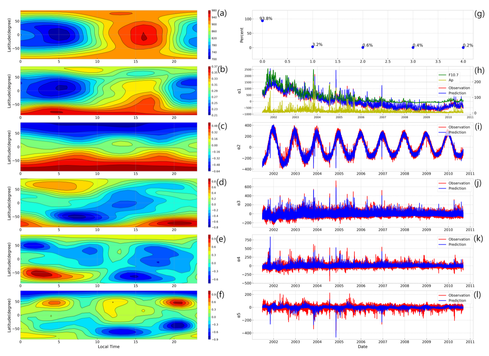
We decomposed the exospheric temperature from CHAMP and GRACE satellites to the mean field and five EOFs as a function of geographic latitude and local time. Figure 3a displays the mean field, the average state, and its maximum and minimum are about 950 K and 700 K at the local time of 16:00 and 5:00, respectively. A significant day–night difference can be discovered in Figure 3b. Furthermore, the highest temperature in EOF1 existed in the Southern high latitudes. The corresponding amplitude in Figure 3h is consistent with the trend of solar activity, having a positive correlation with the Ap index. Thus, EOF1 contains solar and geomagnetic factors, along with some weak season variation. EOF2 is opposite between the Northern and Southern hemispheres, suggesting a potential summer-to-winter asymmetry. As illustrated in Figure 3i, the amplitude of EOF2 exhibits a remarkable and dominant annual variation, and the relative amplitude decreases with time. Figure 3d–f show smaller-scale diurnal and hemispheric variations in the thermosphere. Moreover, the amplitude values in Figure 3j–l have some spikes associated with the geomagnetic activity or other factors, and the details need more and further investigation.
Figure 3g shows the relative contribution of each EOF (from 1st to 5th EOFs) to the total variability of exospheric temperature. The first five EOFs take up 93.8%, 3.2%, 0.6%, 0.4% and 0.2% of the total variability, respectively. In other words, the first five EOFs constitute approximately 98.2% of the total variance, and the five modes obviously dominate the overall exospheric temperature variation. Thus, the modes in Figure 3 are considered to characterize and rebuild the temperature variations.
In order to build a robust ETM, we reconstructed the amplitudes of EOFs in Figure 3h–l through the following equations [13,24,29,30]:
α = T t i m e T S G C ,
T t i m e = a + i = 1 3 ( b 1 i sin 2 π i d 365.25 + b 2 i cos 2 π i d 365.25 ) + j = 1 3 ( c 1 j sin 2 π j h 24 + c 2 j cos 2 π j h 24 ) ,
T S G C = d 1 + s 1 M 10 d 2 + s 2 M 81 c d 3 + g 1 D s t 1 + g 2 D s t 1 D s t 2 + g 3 D s t 1 D s t 3 + g 4 A p a v g .
Here, Ttime is referred to as UT/longitude and seasonal variations, and TSGC denotes the solar and geomagnetic activity effect. In Equation (3), d stands for the day number of the year, meaning the annual, semiannual and terannual variations. h represents the current universal time, including the diurnal, semidiurnal and terdiurnal variations. The M10 and M81c represent daily M10.7 for the previous day, and the 81-day averaged value with centering at the current day. Apavg is the daily averaged 3 h Ap index, and the Disturbance Storm Time (Dst) index is introduced to indicate the temperature response of the storm time in the thermosphere [1]. Dst1 is the transformed Dst index for the current time, and Dstk (k = 2, 3) is for the transformed Dst index every 3 h since 6 h earlier than the current universal time. The coefficients in Equations (3) and (4) are obtained using linear regression. The parameterized results, provided in Figure 3h–l, have correlation coefficients of 0.99, 0.99, 0.87, 0.75 and 0.66 with the observations, respectively. Obviously, Equations (2)–(4) can represent the amplitude values effectively.
Subsequently, by combining Equations (1)–(4), a new ETM is developed as a function of universal time, day number and solar and geomagnetic activities. In the next section, we will examine the ETM and simulate the spatial and temporal variations of the thermosphere. To assess model/data agreement, the Mean Percent Error (MPE) and RMSE are applied to compute the mean and standard deviation of the model-to-data ratios:
M P E = 1 N i = 1 N f m , i f o , i 1 ,
R M S E = 1 N i = 1 N ( f m , i f o , i 1 ) 2 .
Here, the subscripts m and o, respectively, correspond to the model and observation, and f denotes the exospheric temperature or thermospheric density.

3. Results

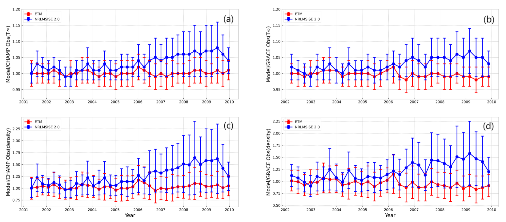
Figure 4a shows the seasonal-averaged ratios along with the standard deviation between the exospheric temperature from the model and CHAMP data. It is evident that the ratios of the NRLMSIS 2.0 model are usually larger than unity, and this empirical model overestimates the exospheric temperature during 2006–2009. However, the ratios between the ETM and CHAMP data remain at around 1, even under low solar activity conditions. In addition, the results are similar for GRACE in Figure 4b. For the thermospheric density in Figure 4c,d, the ratio between the NRLMSIS 2.0 and CHAMP and GRACE data goes up to the value of ~1.6 in 2008, and the RMSE is greater than 0.7. Comparatively, the errors of the ETM prediction are less than 20%, and its RMSE is also significantly contractive. Noteworthy, Figure 4c,d show that the NRLMSIS 2.0 model predictions are generally consistent with the CHAMP and GRACE density measurements in 2002–2006; however, there is an obvious discrepancy seen between them in 2006–2010. The seasonal-averaged ratios between the NRLMSIS 2.0 density predictions and the observations generally are more than 1.25, which indicates that the NRLMSIS 2.0 model overestimates the thermospheric density under low solar activity. Overall, the RMSE for these two models is 24.11% and 41.42%, respectively. Our ETM can represent the exospheric temperature and thermospheric density better than the NRLMSIS 2.0 model.
The ETM is expected to be in better agreement with CHAMP and GRACE results; because of that, the same data are used to develop this model. Therefore, we will use SWARM-C and GRACE-FO data to validate the ETM independently. Obviously, the covered time and height of both satellites are different from CHAMP and GRACE satellites, and the results should be more convincing. Figure 5 presents the scatter plot of our ETM and NRLMSIS 2.0 model predictions versus the SWARM-C and GRACE-FO results, which show that the ETM results are expected to be in better agreement with the SWARM-C observations, but the NRLMSIS 2.0 overestimates the densities significantly under the low density period. Additionally, the MPE of our ETM and NRLMSIS 2.0 model are 4.47% and 22.93%, and the RMSE are 26.45% and 39.52%, respectively, which indicates that the ETM model can reproduce the SWARM-C measurements better than NRLMSIS 2.0 model, and the RMSE has been reduced by approximately 33%. Similarly, the ETM can reproduce the thermospheric densities along the GRACE-FO orbits much better than this NRLMSIS 2.0 model. In addition, the NRLMSIS 2.0 empirical model is greater than the observations during the whole period. Additionally, the MPE and RMSE of our ETM are 1.91% and 26.17%, but they are 32.11% and 44.41% for the NRLMSIS 2.0 model. Figure 5 confirms that our ETM has better performance for thermospheric density prediction than the NRLMSIS 2.0 model.
Figure 6 provides the statistical deviations and relative errors of thermospheric density between the models and SWARM-C and GRACE-FO observations. As seen in Figure 6a, the thermospheric density from the ETM and NRLMSIS 2.0 models both are generally consistent with the SWARM-C density observations in 2014–2017. Similarly, the ETM predictions are in good agreement with SWARM-C observations for the period of 2017–2020; however, there is an obvious discrepancy between the observations and the predictions of the NRLMSIS 2.0 model, which overestimates the density during this period. Moreover, there are many spikes in the ETM predictions, which indicates that the ETM will slightly overestimate the density response during the geomagnetic storm. Furtherly, the feature can be seen from the evaluation indicators clearly shown in Figure 6b, in which the averaged deviation and RMSE of these one-hour means are 4.47% and 26.5%, the same as those provided Figure 5, for the ETM, while they are 22.9% and 39.5% for NRLMSISE 2.0. A further comparison is presented for GRACE-FO in Figure 6c,d. The ETM results are in good agreement with the GRACE-FO observations; however, the NRLMSIS 2.0 model overestimates the densities under the low solar activity condition. This demonstrates that prediction using the ETM model was successful, especially during low solar activity.
Figure 7 depicts the seasonal variations of exospheric temperature from our ETM. Both in the daytime and night-time, the exospheric temperature at the middle and high latitudes exhibit obvious annual variation, with larger temperatures in local summer months. Moreover, the feature is similar under different solar activity conditions, but the absolute magnitude of seasonal variations generally increases with solar activity. Furthermore, the seasonal amplitudes at southern and northern high latitudes are approximately 50% and 30%, showing remarkable hemispheric asymmetry. In total, the features are coincident with the results of Lei and Weng [15,24].
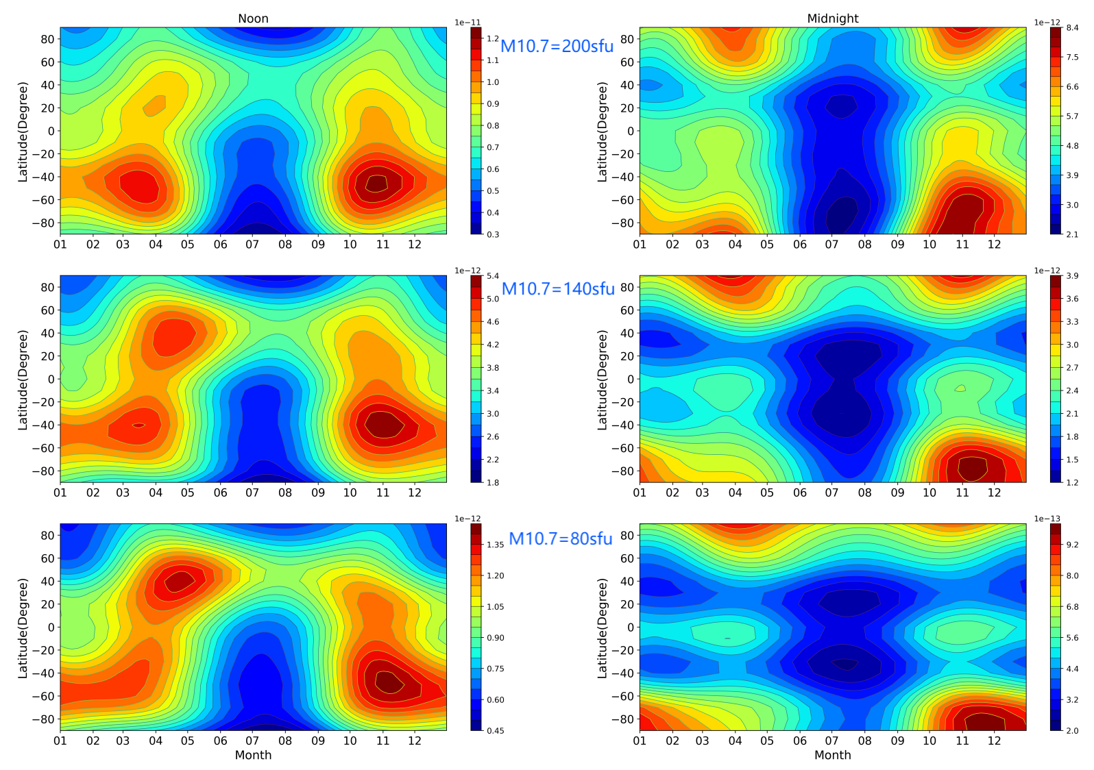
Figure 8 illustrates the seasonal variations of thermospheric density at 400 km predicated from our ETM for the aid of the NRLMSIS 2.0 model. In the daytime and night-time, densities at low and middle latitudes both exhibit obvious semiannual variations, with a maximum around the equinox. In addition, the thermospheric densities around the September equinox at the southern crest are larger than that in the northern hemisphere, and this feature persists under all solar activity conditions. Moreover, the daytime density has a striking ETA feature around the equinox, with a more prominent feature during the Spring months. In the night-time, the Midnight Density Maximum (MDM) around the equator is more visible under middle and low solar activity conditions. In addition, the distribution of Figure 7 is consistent with the results of Lei et al. (2012) and Weng et al. (2017; 2018), the thermospheric density has obvious hemispheric asymmetry, and the amplitudes of density at southern and northern high latitudes are over 200% and 100%, respectively [15,24,31].

4. Conclusions

In this study, the CHAMP and GRACE density measurements during 2002–2010 were used to derive the exospheric temperature with the help of the NELMSIS 2.0 model, and from the decomposition results of the exospheric temperature data, we found that the first five EOFs can capture 98.2% of the exospheric temperature variation. These EOFs take the diurnal variation and hemispheric asymmetry, while the corresponding amplitudes vary with seasonal variation, solar and geomagnetic activities. Then, the ETM was constructed by reconstructing the first five basis function amplitude, and the ETM and NRLMSIS 2.0 model were verified by SWARM-C and GRACE-FO density measurements independently. Overall, our ETM can reproduce the observations much better than the NRLMSIS 2.0 model, especially during the low solar activity period. Furthermore, our ETM can accurately represent the ETA, seasonal variation and the hemispheric asymmetry of the thermospheric density.

Author Contributions

Conceptualization: X.Z., L.W. and X.Y.; methodology and software: X.Y. and S.Y.; writing—original draft: X.Y. and L.W.; writing—review: X.Z., S.Y. and L.W.; funding acquisition, L.W.; data curation: X.Z. and S.Y.; formal analysis: X.Y. All authors have read and agreed to the published version of the manuscript.

Funding

This work was supported by the National Natural Science Foundation of China, grant number 42104162.

Data Availability Statement

Thermospheric density data from CHAMP, GRACE and SWARM-C satellites are available at http://thermosphere.tudelft.nl/ (accessed on 11 May 2021). The Dst index was obtained from https://wdc.kugi.kyoto-u.ac. jp/dstae/index.html (accessed on 5 January 2022). The composite MgII proxy was obtained from http://www.iup.uni-bremen.de/gome/gomemgii.html (accessed on 11 May 2021).

Acknowledgments

The authors are grateful to the sponsors and operators of the CHAMP, GRACE and SWARM missions; the authors would like to give thanks to Li for providing the drag-derived GRACE-FO densities, and the method of retrieving the density was proposed in this study (Li et al., 2017, https://doi.org/10.1007/s11430-016-9052-1, accessed on 19 July 2021).

Conflicts of Interest

The authors declare no conflict of interest.

References

  1. Bowman, B.R.; Tobiska, W.K.; Marcos, F.A.; Huang, C.Y.; Lin, C.S.; Burke, W.J. A new empirical thermospheric density model JB2008 using new solar and geomagnetic indices. In Proceedings of the AIAA/AAS Astrodynamics Specialist Conference and Exhibit, Honolulu, HI, USA, 18–21 August 2008. [Google Scholar]
  2. Bruinsma, S. The DTM-2013 thermosphere model. J. Space Weather Space Clim. 2015, 5, A1. [Google Scholar] [CrossRef] [Green Version]
  3. Hedin, A.E. Extension of the MSIS Thermosphere Model into the middle and lower atmosphere. J. Geophys. Res. Space Phys. 1991, 96, 1159–1172. [Google Scholar] [CrossRef]
  4. Kong, Q.; Chen, Y.; Fang, W.; Wang, G.; Li, C.; Wang, T.; Bai, Q.; Han, J. Analysis of Space-Borne GPS Data Quality and Evaluation of Precise Orbit Determination for COSMIC-2 Mission Based on Reduced Dynamic Method. Remote Sens. 2022, 14, 3544. [Google Scholar] [CrossRef]
  5. March, G.; Doornbos, E.N.; Visser, P.N.A.M. High-fidelity geometry models for improving the consistency of CHAMP, GRACE, GOCE and Swarm thermospheric density data sets. Adv. Space Res. 2019, 63, 213–238. [Google Scholar] [CrossRef]
  6. Mehta, P.M.; Linares, R. A methodology for reduced order modeling and calibration of the upper atmosphere. Space Weather 2017, 15, 1270–1287. [Google Scholar] [CrossRef]
  7. Picone, J.M.; Hedin, A.E.; Drob, D.P.; Aikin, A.C. NRLMSISE-00 empirical model of the atmosphere: Statistical comparisons and scientific issues. J. Geophys. Res. Space Phys. 2002, 107, SIA 15-11–SIA 15-16. [Google Scholar] [CrossRef]
  8. Jacchia, L.G. New Static Models of the Thermosphere and Exosphere with Empirical Temperature Profiles. SAO Special Report 313; Smithsonian Astrophysical Observator: Cambridge, MA, USA, 1970. [Google Scholar]
  9. Doornbos, E.; van den Ijssel, J.; Luhr, H.; Forster, M.; Koppenwallner, G. Neutral Density and Crosswind Determination from Arbitrarily Oriented Multiaxis Accelerometers on Satellites. J. Spacecr. Rocket. 2010, 47, 580–589. [Google Scholar] [CrossRef] [Green Version]
  10. Emmert, J.T. Thermospheric mass density: A review. Adv. Space Res. 2015, 56, 773–824. [Google Scholar] [CrossRef]
  11. Sun, Y.; Wang, B.; Meng, X.; Tang, X.; Yan, F.; Zhang, X.; Bai, W.; Du, Q.; Wang, X.; Cai, Y.; et al. Analysis of Orbital Atmospheric Density from QQ-Satellite Precision Orbits Based on GNSS Observations. Remote Sens. 2022, 14, 3873. [Google Scholar] [CrossRef]
  12. Wise, J.O.; Burke, W.J.; Sutton, E.K. Globally averaged exospheric temperatures derived from CHAMP and GRACE accelerometer measurements. J. Geophys. Res. Space Phys. 2012, 117, A04312. [Google Scholar] [CrossRef]
  13. Ruan, H.; Lei, J.; Dou, X.; Liu, S.; Aa, E. An Exospheric Temperature Model Based On CHAMP Observations and TIEGCM Simulations. Space Weather 2018, 16, 147–156. [Google Scholar] [CrossRef]
  14. Weimer, D.R.; Sutton, E.K.; Mlynczak, M.G.; Hunt, L.A. Intercalibration of neutral density measurements for mapping the thermosphere. J. Geophys. Res. Space Phys. 2016, 121, 5975–5990. [Google Scholar] [CrossRef] [Green Version]
  15. Weng, L.; Lei, J.; Sutton, E.; Dou, X.; Fang, H. An exospheric temperature model from CHAMP thermospheric density. Space Weather 2017, 15, 343–351. [Google Scholar] [CrossRef]
  16. Weimer, D.R.; Mehta, P.M.; Tobiska, W.K.; Doornbos, E.; Mlynczak, M.G.; Drob, D.P.; Emmert, J.T. Improving Neutral Density Predictions Using Exospheric Temperatures Calculated on a Geodesic, Polyhedral Grid. Space Weather 2020, 18, e2019SW002355. [Google Scholar] [CrossRef] [Green Version]
  17. Weimer, D.R.; Tobiska, W.K.; Mehta, P.M.; Licata, R.J.; Drob, D.P.; Yoshii, J. Comparison of a Neutral Density Model With the SET HASDM Density Database. Space Weather 2021, 19, e2021sw002888. [Google Scholar] [CrossRef]
  18. Licata, R.J.; Mehta, P.M.; Weimer, D.R.; Tobiska, W.K. Improved Neutral Density Predictions Through Machine Learning Enabled Exospheric Temperature Model. Space Weather 2021, 19, e2021sw002918. [Google Scholar] [CrossRef]
  19. Siemes, C.; de Teixeira da Encarnação, J.; Doornbos, E.; van den Ijssel, J.; Kraus, J.; Pereštý, R.; Grunwaldt, L.; Apelbaum, G.; Flury, J.; Holmdahl Olsen, P.E. Swarm accelerometer data processing from raw accelerations to thermospheric neutral densities. Earth Planets Space 2016, 68, 92. [Google Scholar] [CrossRef] [Green Version]
  20. Voss, K.A.; Famiglietti, J.S.; Lo, M.; Linage, C.; Rodell, M.; Swenson, S.C. Groundwater depletion in the Middle East from GRACE with implications for transboundary water management in the Tigris-Euphrates-Western Iran region. Water Resour. Res. 2013, 49, 904–914. [Google Scholar] [CrossRef] [Green Version]
  21. Othman, A.; Abdelrady, A.; Mohamed, A. Monitoring Mass Variations in Iraq Using Time-Variable Gravity Data. Remote Sens. 2022, 14, 3346. [Google Scholar] [CrossRef]
  22. Weng, L.; Lei, J.; Zhong, J.; Dou, X.; Fang, H. A Machine-Learning Approach to Derive Long-Term Trends of Thermospheric Density. Geophys. Res. Lett. 2020, 47, e2020GL087140. [Google Scholar] [CrossRef]
  23. Emmert, J.T.; Drob, D.P.; Picone, J.M.; Siskind, D.E.; Jones, M.; Mlynczak, M.G.; Bernath, P.F.; Chu, X.; Doornbos, E.; Funke, B.; et al. NRLMSIS 2.0: A Whole-Atmosphere Empirical Model of Temperature and Neutral Species Densities. Earth Space Sci. 2020, 7, e2020EA001321. [Google Scholar] [CrossRef]
  24. Lei, J.; Matsuo, T.; Dou, X.; Sutton, E.; Luan, X. Annual and semiannual variations of thermospheric density: EOF analysis of CHAMP and GRACE data. J. Geophys. Res. Space Phys. 2012, 117, A01310. [Google Scholar] [CrossRef] [Green Version]
  25. Calabia, A.; Jin, S. New modes and mechanisms of thermospheric mass density variations from GRACE accelerometers. J. Geophys. Res. Space Phys. 2016, 121, 11191–111212. [Google Scholar] [CrossRef]
  26. Delforge, D.; de Viron, O.; Durand, F.; Dehant, V. The Global Patterns of Interannual and Intraseasonal Mass Variations in the Oceans from GRACE and GRACE Follow-On Records. Remote Sens. 2022, 14, 1861. [Google Scholar] [CrossRef]
  27. Matsuo, T.; Forbes, J.M. Principal modes of thermospheric density variability: Empirical orthogonal function analysis of CHAMP 2001-2008 data. J. Geophys. Res. Space Phys. 2010, 115, A07309. [Google Scholar] [CrossRef]
  28. Sutton, E.K.; Cable, S.B.; Lin, C.S.; Qian, L.; Weimer, D.R. Thermospheric basis functions for improved dynamic calibration of semi-empirical models. Space Weather 2012, 10, S10001. [Google Scholar] [CrossRef] [Green Version]
  29. Matsuo, T.; Fedrizzi, M.; Fuller-Rowell, T.J.; Codrescu, M.V. Data assimilation of thermospheric mass density. Space Weather 2012, 10, S05002. [Google Scholar] [CrossRef]
  30. Liu, Z.; Fang, H.; Hoque, M.M.; Weng, L.; Yang, S.; Gao, Z. A New Empirical Model of NmF2 Based on CHAMP, GRACE, and COSMIC Radio Occultation. Remote Sensing 2019, 11, 1386. [Google Scholar] [CrossRef] [Green Version]
  31. Weng, L.; Lei, J.; Doornbos, E.; Fang, H.; Dou, X. Seasonal variations of thermospheric mass density at dawn/dusk from GOCE observations. Ann. Geophys. 2018, 36, 489–496. [Google Scholar] [CrossRef]
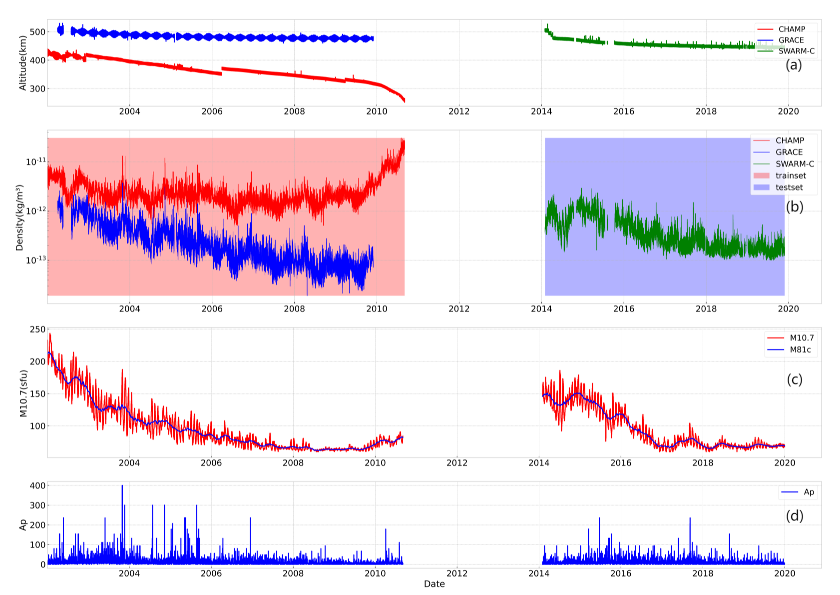
Figure 1. (a) The altitudes of CHAMP (red line), GRACE-A (blue line), SWARM-C (green line) and GRACE-FO (yellow line), (b) thermospheric density measured by the three satellites, (c) daily solar radio flux M10.7 (red line), 81-day average of solar M10.7c (blue line) and (d) geomagnetic activity Ap index.
Remotesensing 14 05198 g001
Figure 2. (a) Daily exospheric temperatures derived from CHAMP and GRACE satellites during 2002–2010, and (b) their statistical results are also shown.
Remotesensing 14 05198 g002
Figure 3. (a) The mean exospheric temperature, and (bf) the first five EOFs as a function of local time and latitude. (g) The relative contribution of each EOF to the total variability of exospheric temperature. (hl) The amplitudes (blue lines) and their fitting results (red lines).
Remotesensing 14 05198 g003
Figure 4. Seasonal ratios and standard deviation between the exospheric temperature from two models and CHAMP (a) and GRACE (b) results; Seasonal ratios and standard deviation between the density from two models and CHAMP (c) and GRACE (d) measurements.
Remotesensing 14 05198 g004
Figure 5. Scatter plots of thermospheric density from SWARM-C (top) and GRACE-FO data (bottom). Left: ETM; Right: NRLMSIS 2.0 model.
Remotesensing 14 05198 g005
Figure 6. (a) two-hours averaged mass density from SWARM-C satellite (red line), ETM results (green line), NRLMSISE 2.0 model (blue line) and (b) the statistic distribution of relative errors of one-hour averaged mass density between SWARM-C observations and ETM results (green line) and NRLMSIS 2.0 model results (blue line); (c) and (d) same as (a) and (b), but for the GRACE-FO satellite.
Remotesensing 14 05198 g006
Figure 7. Seasonal variations of exospheric temperature from our ETM at noon (left) and midnight (right) under different solar activity levels.
Remotesensing 14 05198 g007
Figure 8. Same as Figure 7, but for the thermospheric density at 400 km.
Remotesensing 14 05198 g008
Publisher’s Note: MDPI stays neutral with regard to jurisdictional claims in published maps and institutional affiliations.