Article

The Simultaneous Prediction of Soil Properties and Vegetation Coverage from Vis-NIR Hyperspectral Data with a One-Dimensional Convolutional Neural Network: A Laboratory Simulation Study

1
State Key Laboratory of Soil and Sustainable Agriculture, Institute of Soil Science, Chinese Academy of Sciences, Nanjing 210008, China
2
College of Advanced Agricultural Sciences, University of Chinese Academy of Sciences, Beijing 100049, China
*
Author to whom correspondence should be addressed.
Remote Sens. 2022, 14(2), 397; https://doi.org/10.3390/rs14020397
Submission received: 29 November 2021 / Revised: 31 December 2021 / Accepted: 12 January 2022 / Published: 15 January 2022
(This article belongs to the Section AI Remote Sensing)

Abstract

:
Remote sensing of land surface mostly obtains a mixture of spectral information of soil and vegetation. It is thus of great value if soil and vegetation information can be acquired simultaneously from one model. In this study, we designed a laboratory experiment to simulate land surface compositions, including various soil types with varying soil moisture and vegetation coverage. A model of a one-dimensional convolutional neural network (1DCNN) was established to simultaneously estimate soil properties (organic matter, soil moisture, clay, and sand) and vegetation coverage based on the hyperspectral data measured in the experiment. The results showed that the model achieved excellent predictions for soil properties (R2 = 0.88–0.91, RPIQ = 4.01–5.78) and vegetation coverage (R2 = 0.95, RPIQ = 7.75). Compared with the partial least-squares regression (PLSR), the prediction accuracy of 1DCNN improved 42.20%, 45.82%, 43.32%, and 36.46% in terms of the root-mean-squared error (RMSE) for predicting soil organic matter, sand, clay, and soil moisture, respectively. The improvement might be caused by the fact that the spectral preprocessing and spectral features useful for predicting soil properties were successfully identified in the 1DCNN model. For the prediction of vegetation coverage, although the prediction accuracy by 1DCNN was excellent, its performance (R2 = 0.95, RPIQ = 7.75, RMSE = 3.92%) was lower than the PLSR model (R2 = 0.98, RPIQ = 12.57, RMSE = 2.41%). These results indicate that 1DCNN can simultaneously predict soil properties and vegetation coverage. However, the factors such as surface roughness and vegetation type that could affect the prediction accuracy should be investigated in the future.

Graphical Abstract

1. Introduction

Remote sensing of vegetation cover and soil is key to land degradation assessment. Suitable remote sensing approaches should be investigated for both vegetation and soil-related properties [1]. However, previous studies have mostly concentrated on remote sensing of the soil or vegetation properties, and few have simultaneously focused on vegetation and soil-related properties. For example, Castaldi et al. [2] used hyperspectral and multispectral satellite data to predict soil organic matter (SOM) and soil texture. Ayehu et al. [3] developed a soil moisture prediction model using remote sensing data acquired from Sentinel-1 Synthetic-Aperture Radar, Moderate-Resolution Imaging Spectroradiometer, and the Shuttle Radar Topographic Mission. Wiesmair et al. [4] estimated vegetation cover based on two vegetation indices, the normalized difference vegetation index and the modified soil adjusted vegetation index, which were derived from multispectral WorldView-2 data. Spectral information in pixels of a satellite image is usually a mixture of spectra of vegetation and soil [5,6]. Therefore, developing one model for retrieving both vegetation and soil-related properties simultaneously is worth investigating because of the improvement in modeling efficiency.
Machine learning (ML) methods have been used to retrieve vegetation cover and soil properties separately. Gholizadeh et al. [7] reported that the memory-based learning method performed better than the partial least-squares regression (PLSR), support vector machine regression (SVR), and boosted regression tree to predict soil texture with hyperspectral data. Yang et al. [8] evaluated four calibration models such as PLSR, least-squares support vector machines, extreme learning machines (ELMs), and cubist, to predict SOM based on visible and near-infrared (Vis–NIR) spectral data. The results showed that the ELM with the genetic algorithm was the best model for predicting SOM. Zhu et al. [9] found that the PLSR model could provide an accurate and stable prediction of soil moisture content (SMC). Dennison et al. [10] found that the PLSR model using the simulated hyperspectral data achieved the lowest average validation root-mean-squared error of coverage for three vegetation types. Recently, the coupling of Vis–NIR hyperspectral data and deep learning methods has demonstrated great potential in predicting soil properties and achieved higher predictive accuracy than traditional ML methods such as PLSR [11,12,13].
However, simultaneous prediction of soil and vegetation properties is a demanding task, which requires the prediction model could simultaneously learn multiple tasks. Recently, the convolutional neural network (CNN) has been used to predict multiple soil properties simultaneously because of its effective feature extraction structure and strong modeling capability [14,15]. For example, Padarian et al. [16] demonstrated that the two-dimensional CNN (2DCNN) could be used to simultaneously predict six soil properties (organic carbon, clay, sand, cation exchange capacity, pH, and total nitrogen) from hyperspectral data. Tsakiridis et al. [15] applied a multichannel, one-dimensional CNN (1DCNN) to predict 10 soil properties (organic carbon, silt, clay, sand content, pH, cation exchange capacity, total nitrogen, calcium carbonate, phosphorus, and extractable potassium) simultaneously with higher accuracy (R2 = 0.42–0.96) than PLSR (R2 = 0.35–0.91), SVR (R2 = 0.39–0.94) and cubist (R2 = 0.39–0.95). Ng et al. [14] reported that the 1DCNN model (R2 = 0.95–0.98) outperformed the 2DCNN model (R2 = 0.90–0.95), and the PLSR model (R2 = 0.87–0.95) for the prediction of several soil properties. The above studies have demonstrated the potential of CNN, especially the 1DCNN model, in predicting soil properties simultaneously, compared with commonly used ML methods. However, previous studies rarely reported the remote sensing of soil properties and vegetation coverage simultaneously using 1DCNN.
Although CNN outperformed the traditional ML methods in many tasks, it is often considered a black box due to the lack of interpretability. Recently, visualization analysis has been introduced to explain how this kind of deep learning methods works [17,18,19]. Generally, the processes associated with CNN could be visualized by filter (kernel) or weight visualization [20], feature visualization, and occlusion sensitivity [19]. For example, weight visualization is helpful to understand how the filters address the input data, and feature visualization could help us understand the features learned by the deep learning model explicitly. In this study, we employed visualization analysis to interpret the features and identify the important wavelengths in 1DCNN.
Therefore, the objectives of this study were (1) to evaluate the ability of the 1DCNN model to simultaneously predict soil properties and vegetation coverage from Vis–NIR hyperspectral data, (2) to compare the results of 1DCNN with the widely used PLSR model, and (3) to visualize the features and identify the important wavelengths of predicting soil properties and vegetation coverage to understand and interpret the 1DCNN model.

2. Materials and Methods

2.1. Experimental Design

A laboratory experiment was conducted to simulate different land surface compositions, including various vegetation coverage and soils with several moisture contents. In this study, a total of 164 soil samples were collected from the Inner Mongolia Autonomous Region, Heilongjiang, Henan, Shandong, Anhui, Jiangsu, Jiangxi, Zhejiang, Hunan, and Fujian provinces of China (Figure 1). All soil samples were sampled by the five-point, blended sampling method, and the sampling depth was 0–20 cm. The collected soil samples covered different parent materials, soil types, topographies, and land uses.
The obtained soil samples were air dried in a drying room and ground (<2 mm). Each soil sample was divided into two parts: one was for the reflectance spectral measurement, and the other was applied to analyze soil properties. In total, 30 soil samples that represented typical soil types in China, including the Aeolian sandy soils of the north, the black soils of the northeast, the fluvo-aquic soils of the North China Plain, the paddy soils of the Middle-Lower Yangtze Plain, and the red soils in southern China were selected to simulate various combinations of different soil types, soil moisture conditions, and vegetation coverage. The remaining soil samples were used to simulate bare soils with different SMCs.
To acquire different SMCs, each soil sample was placed in a black sample box with a diameter of 20 cm and a depth of 1.5 cm, with some uniform small holes lined with filter paper at the bottom. Then, the sample boxes containing the soil samples were placed in a larger container with distilled water to allow the soil to absorb water evenly from the bottom to the top until the soil was saturated with water. The saturated soil samples were placed in a cool and dry place for natural evaporation [21]. During the natural drying process, different SMCs were obtained.
In order to obtain different vegetation coverage, we planted corn in containers in the greenhouse. The fresh corn leaves were collected and cut into different sizes in advance and then were incrementally placed on the soil surface to simulate different percentages of vegetation coverage. We designed a total of 12 coverage levels (an interval of about 5%), with coverage varying from 0% to 60%.

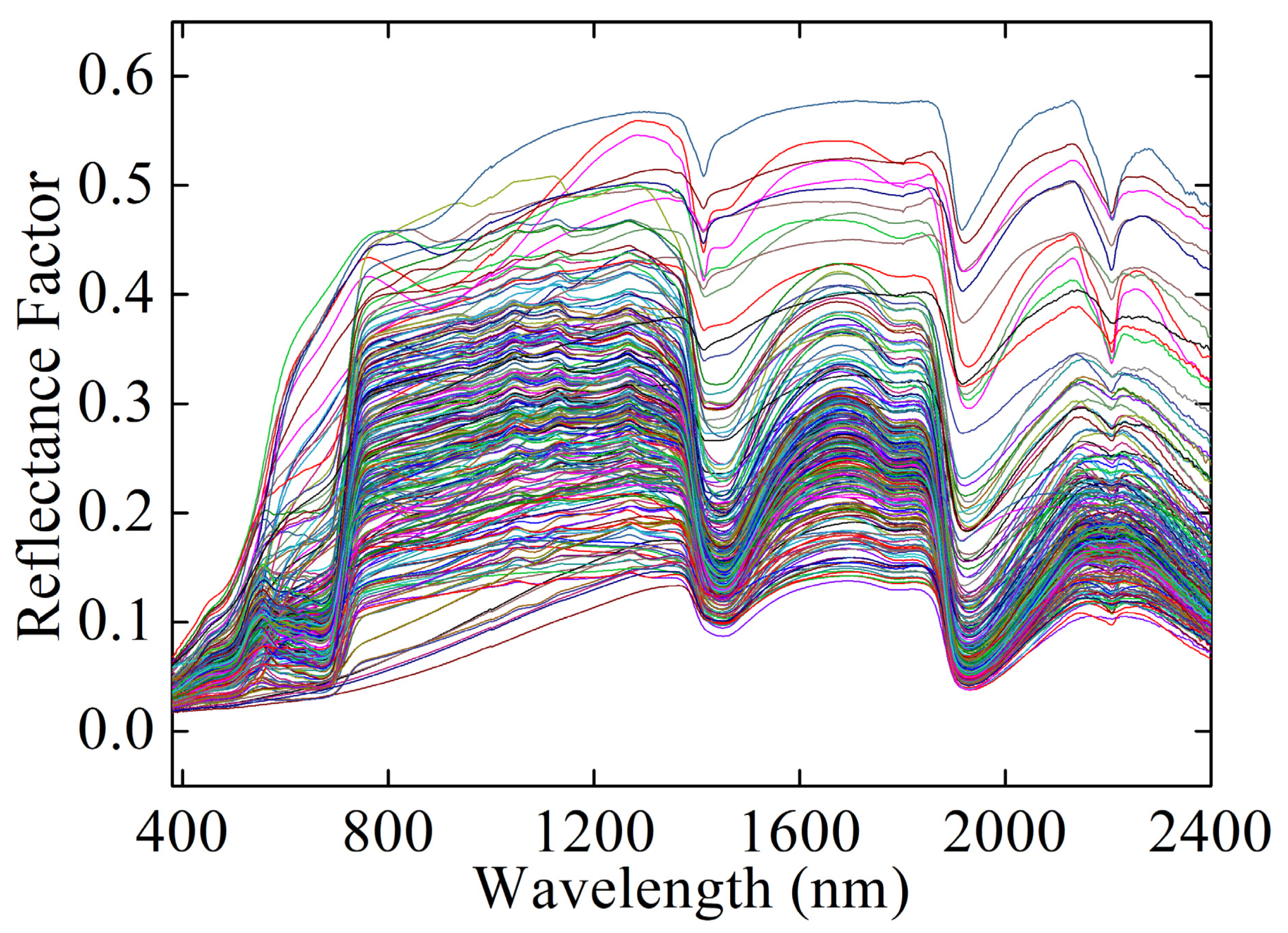
2.2. Spectra Collection

The spectral measurements were implemented in a dark room with an ASD FieldSpec 4 Hi-Res (ASD PANalytical, Boulder, CO, USA) spectroradiometer with a spectral range from 350 nm to 2500 nm. The aperture angle of 25° was chosen and vertically mounted 35 cm above the sample surface, resulting in a field of view of 15.5 cm in diameter. The illumination was provided by two 50-watt quartz halogen lamps with a zenith angle of 45°. A standard white Spectralon panel (25 × 25 cm2) (Labsphere, North Sutton, NH, USA) was used to calibrate the instrument. During the natural evaporation of soil water, the reflectance spectra of all soil samples were measured regularly every about eight hours until the weight of the sample no longer changed. For each spectral measurement (Figure 2), the wet soils were weighed to calculate the corresponding SMC, the fresh corn leaves with different size combinations were only placed in the center of the soil surfaces of the selected 30 typical soil samples to obtain different vegetation coverage, the spectra were measured, and the digital photos were also taken after each spectral measurement to calculate the specific vegetation coverage. Twenty spectra of each sample from four directions were taken to eliminate the effects of shadows.

2.3. Data Preparation

SOM was measured using the modified Walkley–Black method [22]. The clay and sand contents were determined using the hydrometer method [23]. SMC (%) was calculated as the weight of wet soil minus the weight of dry soil, divided by the weight of dry soil multiplied by 100. The mean relative error of SOM, clay, and sand were 2.11%, 2.42%, and 2.85%, respectively, which were calculated based on replicate measurements of four soil samples randomly selected from all samples.
In order to calculate the vegetation coverage, we used the HSV (Hue, Saturation, and Value) color space to extract the vegetation from the previously taken digital photos since it can describe a target’s color independent of the illumination condition [24]. First, the Hough transform [25] was used to extract the regions of interest in batches. Then, the digital photos were converted from RGB into HSV, and a threshold was set to obtain the vegetation binary image. The vegetation coverage was determined by calculating the proportion of vegetation in the binary image. As some corn leaves were placed on the surface of wet soil during the natural evaporation of soil water, the corners of the leaves might be stained with soils, which could cause a minor error in the calculation result of vegetation coverage. However, this error is negligible. The summary statistics of all soil properties and vegetation coverage are shown in Table 1.
A total of 20 spectra of each sample were averaged, and then, the averaged spectrum was determined as the final spectrum of each sample. Only 380–2400 nm wavelengths were utilized for data analysis and modeling because of the low signal-to-noise ratio of the wavelengths at both ends (350–379 nm and 2401–2500 nm, respectively). For the 1DCNN model, the raw spectra were fed into the model. For PLSR modeling, we investigated four spectral pretreatments (i.e., Savitzky–Golay (SG) smoothing, absorbance transform, standard normal variate, and first derivative) and their combinations. We selected the pretreatment of SG smoothing (with a polynomial degree of 2 and a window size of 9), followed by the first derivative to preprocess the spectra based on the prediction results (not shown).
A total of 11,165 spectra including 2503 spectra of bare soils with different SMCs and 8662 mixture spectra of soil–vegetation with different SMCs and vegetation coverage were obtained. The parts of the original spectra are shown in Figure 3. All of the data were randomly divided into a training set (80%, 8932 samples) and a test set (20%, 2233 samples). The random splits were repeated 20 times, with a result of 20 training and test data sets. We built prediction models using each training set and then evaluated model performance using the corresponding test set. Finally, the following evaluation metrics were averaged to evaluate the model performance.

2.4. Models

2.4.1. Partial Least-Squares Regression (PLSR)

PLSR is a linear multivariate statistical analysis method where the data are projected into latent variables (LVs) that maximize the covariance between the independent and predictor variables [26]. It effectively overcomes the problem of multicollinearity, which cannot be solved by ordinary linear regression. A 10-fold cross-validation approach was used to prevent overfitting and find the optimal number of LVs that resulted in the smallest root-mean-squared error (RMSE). The PLSR method was established to compare the performance with the proposed deep learning model in this study.

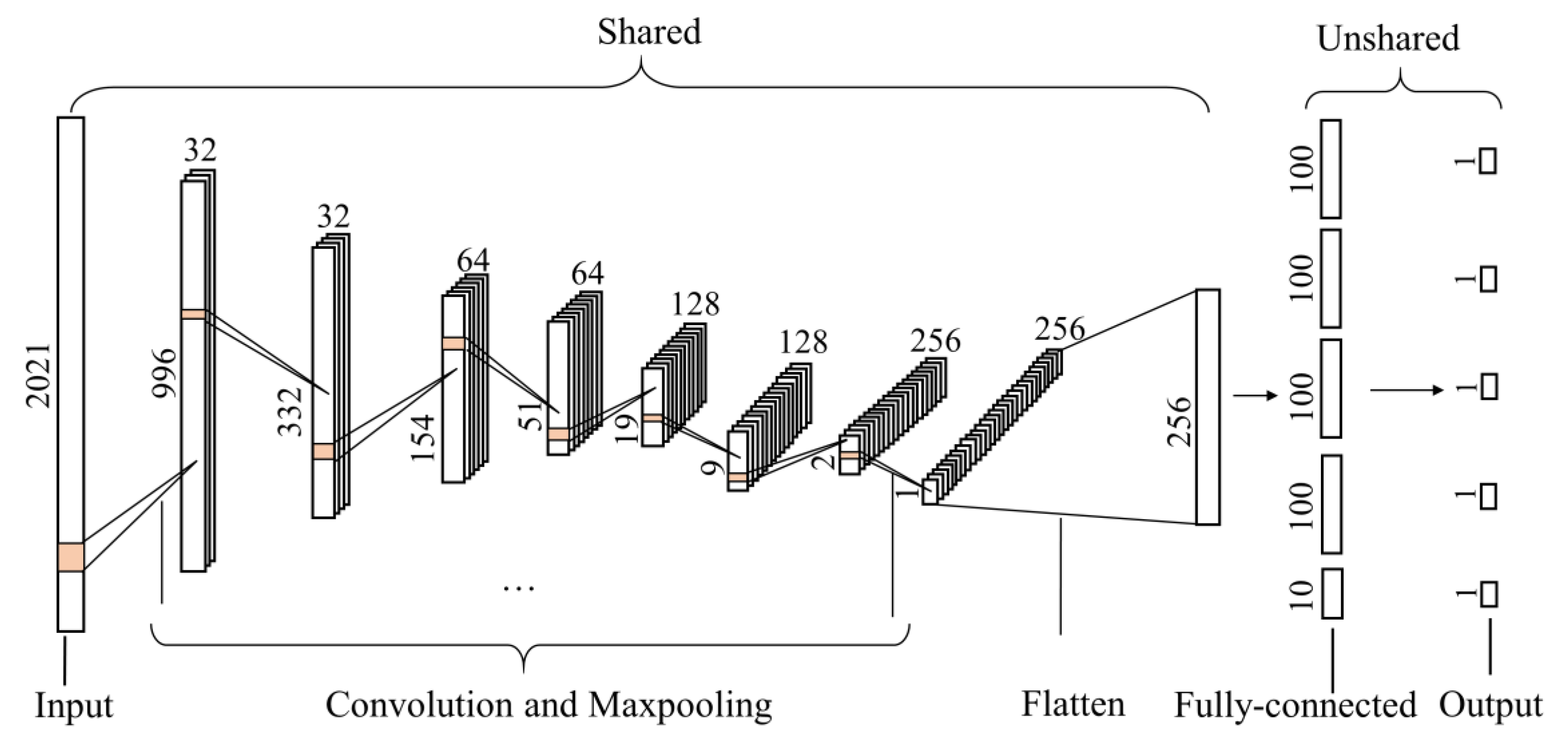
2.4.2. One-Dimension Convolutional Neural Network (1DCNN)

The 1DCNN model has proved effective for soil spectroscopy [15,27,28,29]. It requires one-dimensional data as input and uses a one-dimensional filter to construct convolutional layers. Generally, the 1DCNN model contains an input layer, a convolutional layer, an activation layer, a pooling layer, a flatten layer, a fully connected layer, and an output layer. Firstly, the input layer accepts one-dimensional data. Then, the convolutional layer performs feature extraction and feature mapping on the input data with different-sized convolutional filters, and the activation layer transforms the data after the convolution using a kernel function. Then, the pooling layer used to conduct sparse processing for the feature maps reduces the number of model hyperparameters. After pooling layers, the flatten layer is used to flatten the multidimensional matrix into a vector, and then the vector obtained is fed into the fully connected layer, where each input is connected to each output through a weight.
The 1DCNN model can predict more than one target property simultaneously, which is called multitask learning. In recent years, multitask deep learning has attracted much attention in recognition, classification, detection, and prediction tasks [15,30,31] because it could overcome overfitting issues in single-task learning by regularization effect of the parameter sharing mechanisms [32]. In this study, we used the hard parameter sharing method to perform the 1DCNN for predicting soil properties and vegetation coverage simultaneously, and the selected loss function was the RMSE value. The entire network was trained by the weighted sum loss function of all tasks (i.e., all soil properties and vegetation coverage), calculated as follows:
L = i = 1 n λ i L i
where λ i and L i are the task loss weight and the task-specific loss, respectively.
The multitask-1DCNN model is depicted in Figure 4. Four convolution and max-pooling layers were shared in which a nonlinear activation function named the rectified linear unit (ReLU) [33] in the activation layer was used to allow the nonlinear transformation of the input. Then, a flatten layer was applied to flatten the data into one dimension. Finally, each specific task had a fully connected and output layer with a linear activation function. The parameters of the layers are reported in Table 2.
In this study, the 1DCNN model was trained with a batch size of 128 and a maximum of 500 epochs using the Adam optimizer [34] to minimize the multitasking loss generated by calculating the sum of the product of each task-specific loss and the loss weighting. Besides, a dropout rate of 0.2 and early stopping patience of 15 (epochs without improvement of test loss) [35] were also implemented to prevent overfitting.

2.5. Implementation

The 1DCNN model was implemented on a GPU (NVIDIA Tesla P100-PCIE-16GB) in python 3.5.4 using Keras 2.15 with TensorFlow 1.4.0 as backend. The PLSR algorithm was implemented with the PLS module in python 3.6.1 on the CPU (Intel Core i7 7700k 4.20 GHz CPU with 16 GB of memory). All models were performed on the Windows operating system with Spyder [36] integrated development environment.

2.6. Model Performance

The performance of the models was assessed on the independent test set with the following evaluation metrics: the coefficient of determination (R2), RMSE, and the ratio of performance to interquartile distance (RPIQ). RPIQ takes the variation of observed values and prediction error into account, hence making it less susceptible to the distribution of observed values [37].
R 2 = 1 S S E / S S T
where S S E is the sum of squared errors, and S S T is the total sum of the squared differences of the observed values from the mean.
RMSE = i = 1 n ( y ˜ i y i ) 2 / n
where y ˜ is the predicted value, y is the observed value, and n is the total number of samples.
RPIQ = IQR / RMSE
where IQR is the interquartile range.
Higher R2 and RPIQ, and lower RMSE values indicate better accuracy. In this study, referring to the existing categories [38,39], and based on our data, we defined excellent predictions with R2 ≥ 0.85 and RPIQ ≥ 4.0, good predictions with 0.6 ≤ R2 < 0.85 and 2.0 ≤ RPIQ < 4.0, and poor predictions with R2 < 0.6 and RPIQ < 2.0.

3. Results

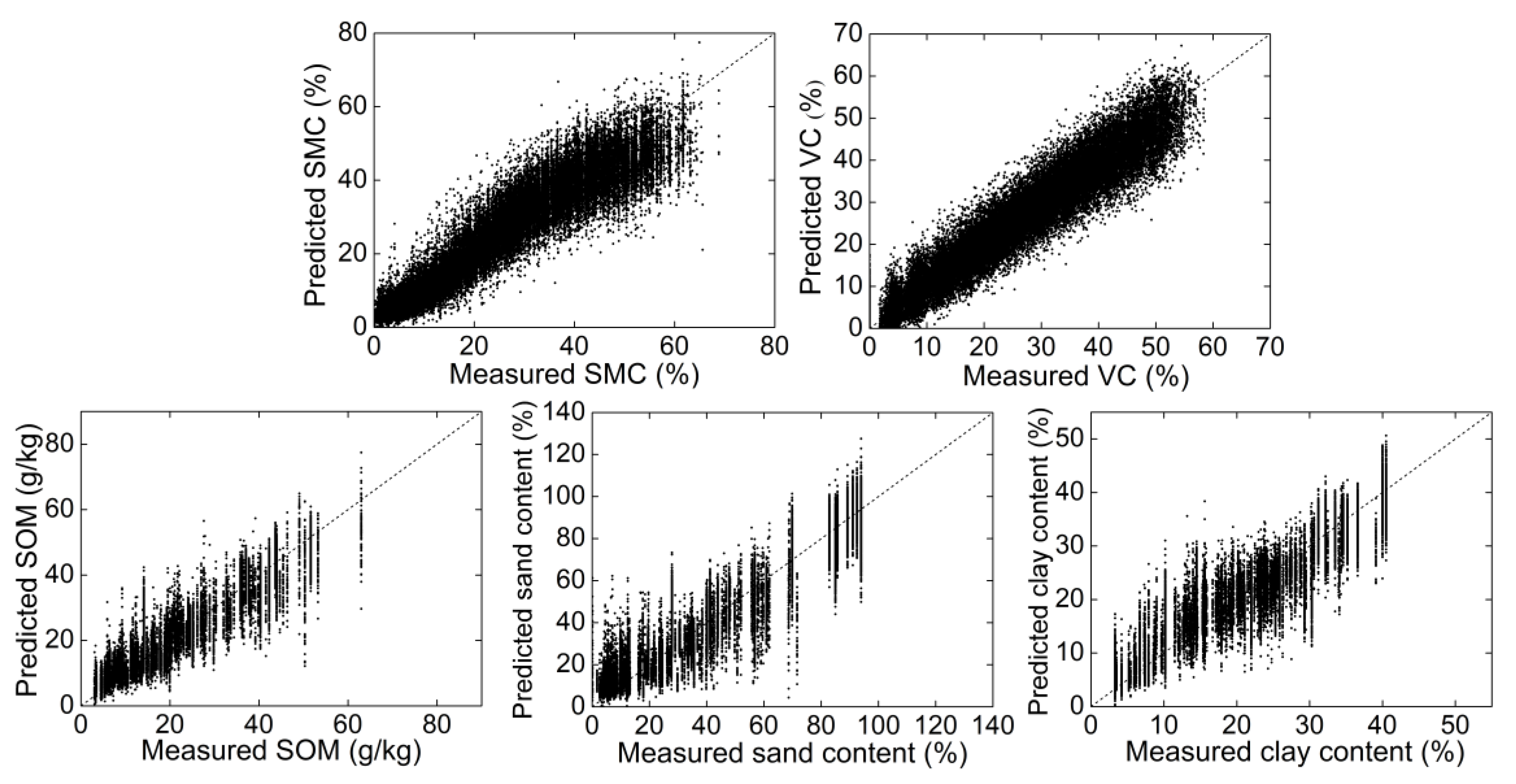
3.1. Results of 1DCNN

The average results of the 20 random independent test sets using the 1DCNN model are shown in Table 3. The results suggested that the 1DCNN model using raw spectra achieved excellent performance for predicting soil properties (0.88 ≤ R2 ≤ 0.91 and 4.01 ≤ RPIQ ≤ 5.78) and vegetation coverage (R2 = 0.95, RPIQ = 7.75). The predicted and measured soil properties and vegetation coverage of 20 randomly selected test sets are plotted in Figure 5. It could be found that the scatter points of SMC and vegetation coverage were closer to the 1:1 line, although the prediction accuracy of SOM, clay, and sand content was also excellent. These results demonstrated the effectiveness of the 1DCNN model to simultaneously predict soil properties and vegetation coverage.

3.2. Comparison between 1DCNN and PLSR

As shown in Table 3, the PLSR model using preprocessed spectra obtained good performance (0.62 ≤ R2 ≤ 0.73 and 2.16 ≤ RPIQ ≤ 3.34) for soil properties and excellent performance for vegetation coverage (R2 = 0.98, RPIQ = 12.57). The 1DCNN model (0.88 ≤ R2 ≤ 0.91 and 4.01 ≤ RPIQ ≤ 5.78) significantly outperformed the PLSR model for the prediction of soil properties. However, we found that the PLSR model had better performance than the 1DCNN model when predicting the vegetation coverage. To further compare the accuracy of the 1DCNN model with the PLSR model, the relative accuracy improvements in the RMSE value were calculated. Compared with the PLSR model, the 1DCNN model achieved relative accuracy improvements of 36.46–45.82% for soil properties. For the vegetation coverage prediction, the PLSR model (RMSE = 2.41%) had an improvement of RMSE, compared with the 1DCNN model (RMSE = 3.92%), although the prediction accuracy of 1DCNN was excellent. Chemometric analysis of spectral data depends on spectral preprocessing such as smoothing, derivatives, and standard normal variate. The 1DCNN with raw spectra achieved higher performance for soil properties and excellent performance for vegetation coverage. These results demonstrated that the 1DCNN model could significantly improve the prediction accuracy of soil properties, except for vegetation coverage, compared with the PLSR model.

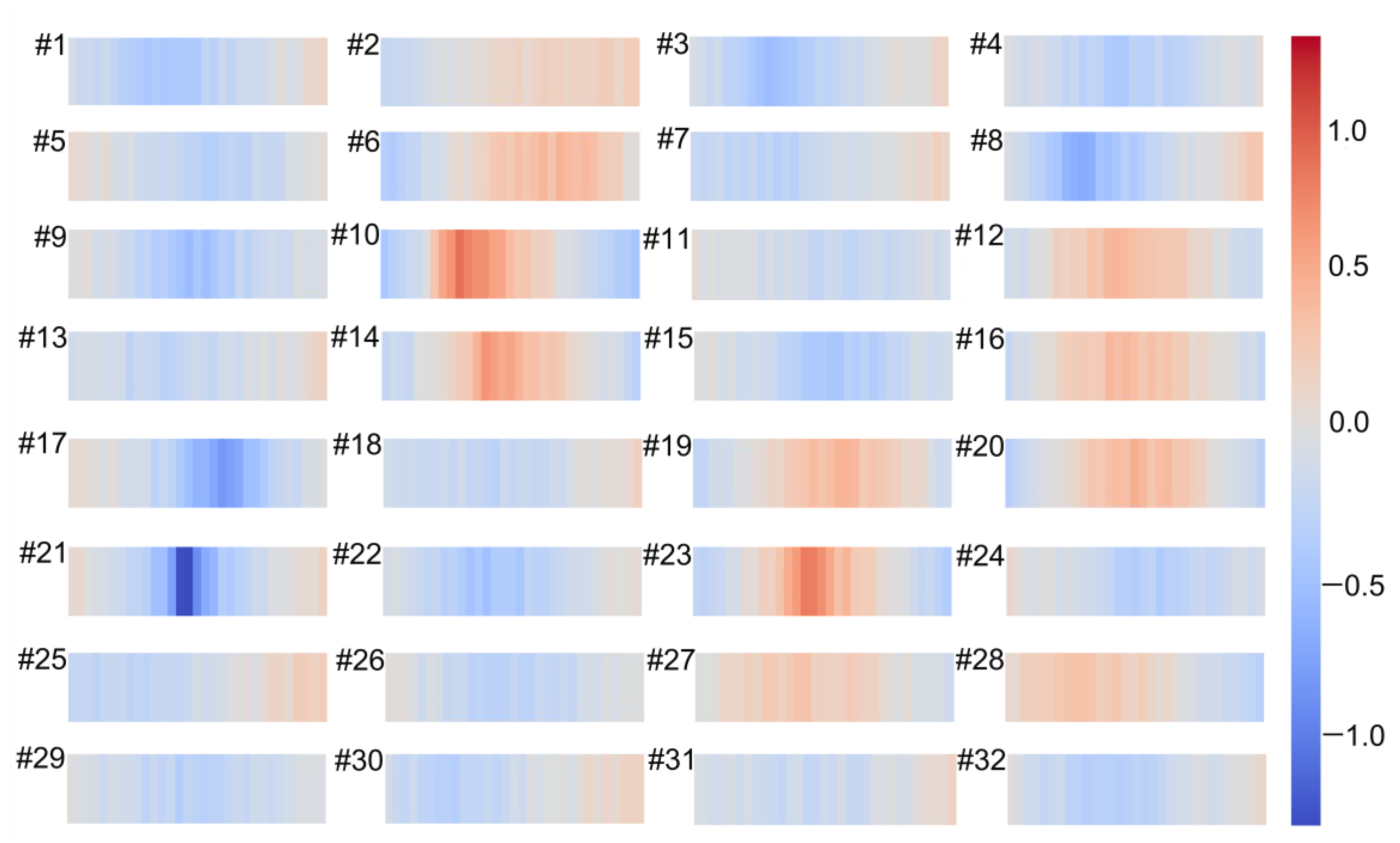
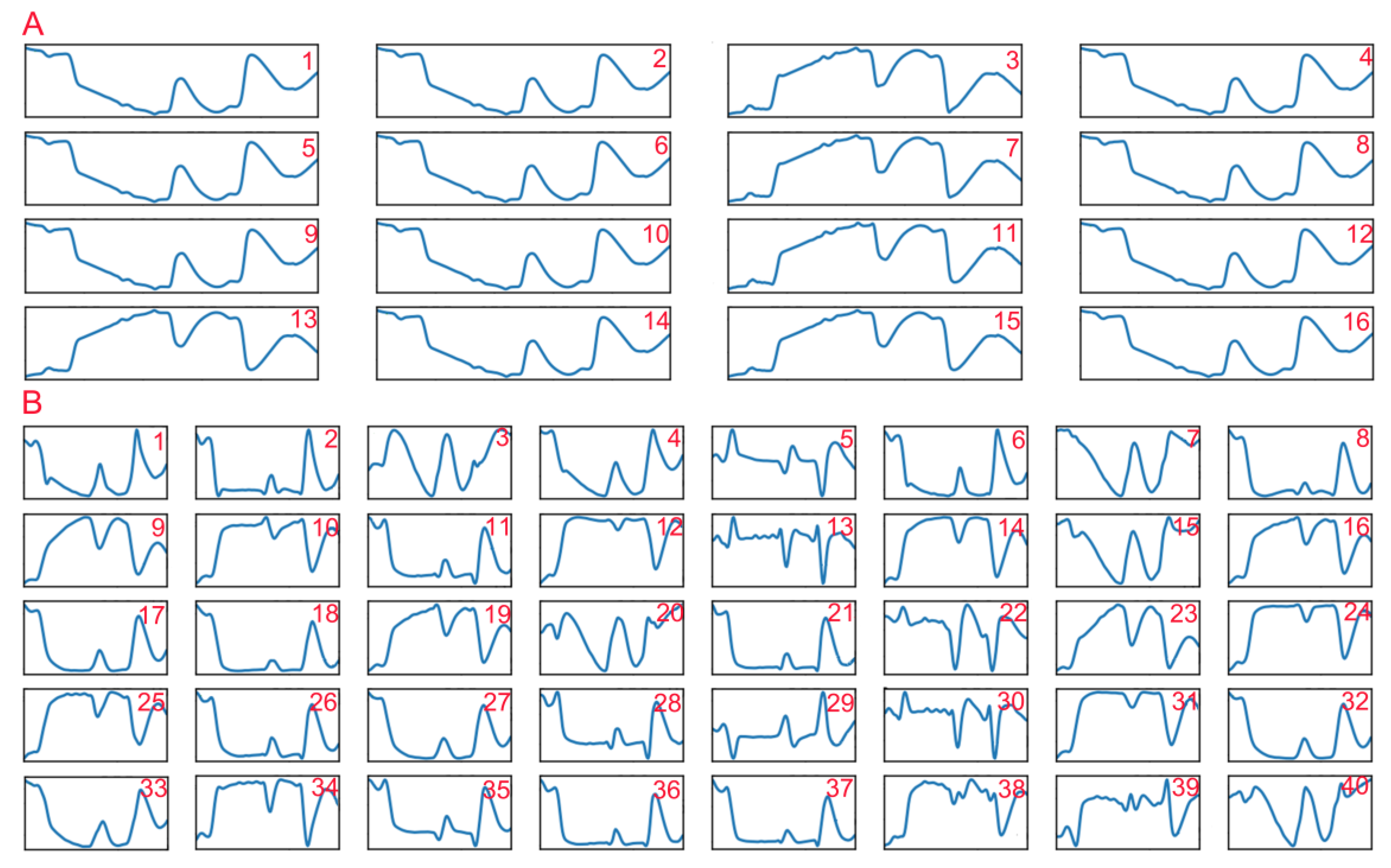
3.3. Visualization of 1DCNN

As is well known, convolution is the process of feature extraction using filters where each filter affects the input in different ways. In order to determine how the filters address the input data, we visualized the weights of the first convolutional layer in the 1DCNN model. The weights of 32 filters in the first convolutional layer are presented in Figure 6. The results showed that the different filters affected the input spectrum in different ways. For example, filters 10, 21, and 23 could identify peaks or troughs, and filter 2 almost showed a gradual process.
In addition, we also visualized the outputs of the first two convolutional layers (Figure 7) to understand what the convolutional layers learned. We found that there were fewer learned features in the first convolutional layer, and these features could be categorized into two types: one was similar to the original average spectrum, and the other resembled the average absorbance spectrum. Compared with the features extracted by the first convolutional layers, the features extracted by the second convolutional layer seemed more abundant and detailed. Some features resembled the original spectra (features 9, 12, 14, 16, 19, 23–25, 31, and 34) and the absorbance spectra (features 1, 2, 4, 6, 8, 17–18, 21, 26–27, 32–33, and 36–37) with some small morphological differences. Some were found to be similar to the first-order derivative spectrum (features 5, 13, 22, and 30), some looked similar to the spectra that were converted to absorbance first and then to first-order derivative (features 29 and 39), and the others seemed abstract. These results suggested that the convolution operation could play a role in spectral preprocessing and also extract some other spectral features, which might help improve the prediction accuracy of 1DCNN.

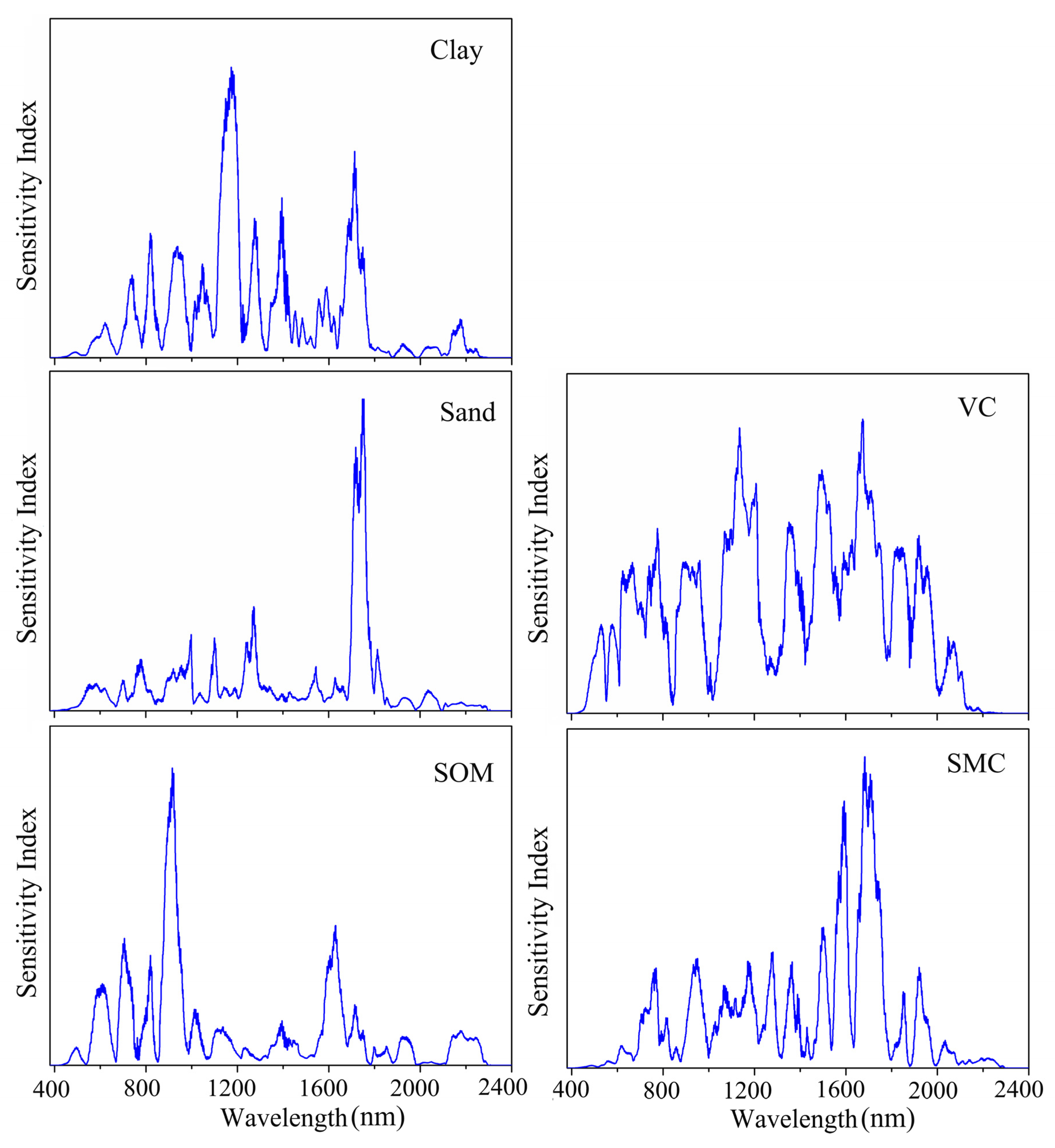
3.4. Determination of Important Wavelengths of 1DCNN

To determine which spectral wavelengths played important roles in the prediction of soil properties and vegetation coverage in the 1DCNN model, a sensitivity analysis based on the variance principle was implemented according to [40]. The results are shown in Figure 8. The important wavelengths to predict SOM were 552–1054 and 1555–1752 nm, and the most important wavelength was around 921 nm. The wavelengths between 547 and 1788 nm were considered significant for predicting clay content. For the prediction of sand content, the important wavelengths identified by the 1DCNN model were 518–1854 nm. It could be found that the important wavelength regions for the prediction of clay and sand content were similar; however, their most important wavelengths were not identical. Wavelengths around 1170 nm were deemed to be the most important for clay prediction, while near 1743 nm were the most important wavelengths to predict sand. The important wavelengths for SMC prediction were mainly distributed in 596–2096 nm, with the two highest peaks at 1683 and 1707 nm, respectively. For the prediction of vegetation coverage, the wavelengths of 462–2125 nm peaked at around 533, 582, 669, 778, 904, 1136, 1358, 1501, 1675, 1842, 1922, and 2077 nm, respectively, were identified to be important. We found that the important wavebands of soil properties overlapped at different degrees.

4. Discussion

In this study, we used a 1DCNN model to simultaneously predict soil properties and vegetation coverage and compared its performance with PLSR. The 1DCNN model significantly outperformed the PLSR counterpart for predicting soil properties. This finding was in line with the results found by Ng et al. [14] and Tsakiridis et al. [15]. However, the PLSR model performed slightly better at predicting vegetation coverage in this study, although the 1DCNN model achieved excellent performance. It is well known that CNN had higher capabilities to deal with complex nonlinear issues because the nonlinear activation function was introduced into the neural network that converted the linear input to a nonlinear output [41,42]. Soil moisture and soil spectra are nonlinearly related [43], resulting in a complicated relationship between other soil properties (SOM, clay, and sand) and spectra reflectance in this study, which could limit the performance of the linear PLSR. Nevertheless, the relationship between the vegetation coverage and reflectance spectra was relatively simple since the vegetation cover in this study was just a single layer of leaf cover, which made the linear PLSR model sufficient to predict vegetation coverage. Thus, it was not necessary to use the CNN model to predict the vegetation coverage. However, various leaf orientations and densities of the three-dimensional vegetation with a distinct layer structure could cause multidirectional reflections of light [44], increasing the complexity of the vegetation reflectance. Consequently, it has not yet been validated whether the PLSR model can still perform well for the vegetation coverage prediction under field conditions.
Compared with the study using CNN to predict soil properties by Padarian et al. [16], the 1DCNN model in our study achieved better performance, with an R2 of 0.88 vs. 0.68 and an RMSE of 3.82% vs. 7.29% for clay, an R2 of 0.89 vs. 0.59 and an RMSE of 8.30% vs. 17% for sand. This might be caused by the dimension difference of the input data. We used the 1D spectra as input in this study, while they used the 2D spectrograms. Ng et al. [14] also demonstrated that 1D spectra input to the CNN model had higher performance than 2D spectrograms. When compared with the study of Tsakiridis et al. [15], who applied a localized, multichannel 1DCNN to predict soil properties, our 1DCNN model performed better for both clay (R2 = 0.88 and RPIQ = 4.65 vs. R2 = 0.86 and RPIQ = 3.75) and sand (R2 = 0.89 and RPIQ = 4.01 vs. R2 = 0.79 and RPIQ = 3.77). A possible reason for this is the higher soil difference in Tsakiridis et al. [15], with approximately 20,000 soil samples encompassing 23 countries of the European Union.
In the literature, many studies have predicted single soil property at a time from one model. Compared with these studies, our 1DCNN model performed better. For example, for SOM, the 1DCNN model (R2 = 0.91 and RMSE = 4.15 g/kg) performed significantly better in our study than the model used by Tsakiridis et al. [45], i.e., a genetic, algorithm-based stacking model (R2 = 0.76 and RMSE = 5.20 g/kg) and that used by Yang et al. [8], which was an ELM model (best R2 = 0.81 and RMSE = 5.17 g/kg). However, our 1DCNN model was not as good as some studies. For example, the prediction accuracy of clay (R2 = 0.88, and RMSE = 3.82%) and sand (R2 = 0.89 and RMSE = 8.30%) was relatively lower than that of Jaconi et al. [46], who used a memory-based learning model with log-ratio transformation to simultaneously estimate clay (R2 = 0.97 and RMSE = 1.85%) and sand (R2 = 0.96 and RMSE = 6.61%) contents. The reason might be that vegetation cover has an impact on the acquisition of soil spectral characteristics, resulting in a slightly lower performance of soil clay and sand in our study.
The performance of models could be affected by soil properties. In our study, the performance of both models in predicting clay and sand contents was relatively lower than SOM. Padarian et al. [16] also reported that the prediction accuracy of clay (R2 = 0.68, RMSE = 7.29%) and sand (R2 = 0.59, RMSE = 17%) was lower than organic carbon (R2 = 0.69, RMSE = 16.82 g/kg). However, in the study of Teixeira et al. [47], clay (best R2 = 0.899, the root-relative-squared error (RRSE) = 32.54%) presented better results than SOM (best R2 = 0.770, RRSE = 47.73%). The reason for these mixed results might be from the difference of soil types among different studies. It should be noted that soil types were more diverse in Padarian et al. [16] and our study, compared with those in Teixeira et al. [47].
We also analyzed the important spectral wavelengths of 1DCNN to predict soil properties and vegetation coverage. For SOM prediction, the most important waveband identified was around 921 nm, which was similar to the results reported by Sung [48] and Lee et al. [49], in which around 910 and 965 nm were considered important for SOM estimation. The most significant wavelength for SOM prediction might be correlated with goethite [50] in this study. We found that the important wavelengths for the prediction of clay and sand contents were 547–1788 nm and 518–1854 nm, respectively. Ng et al. [40] also reported that 500–1800 nm were significant for predicting clay and sand contents in the CNN model. However, the most important wavelength for predicting clay and sand contents was not similar in this study, which was different from those found by Ng et al. [40] in which the most important wavelength shared a high similarity. In this study, the clay and sand content prediction might be related to -OH in clay minerals, iron oxides (primarily hematite and goethite), and organic matter [51]. For SMC prediction, the important wavelengths were distributed in Vis–NIR regions. Nevertheless, NIR regions contributed more to the SMC prediction and had two highest peaks at around 1683 and 1707 nm, which was similar to the results reported by Liu et al. [52], in which 1622 and 1834 nm performed better to estimate soil moisture. The important wavelength regions (462–2125 nm) for the vegetation coverage prediction by 1DCNN had several peak values (at 533, 582, 669, 778, 904, 1136, 1358, 1501, 1675, 1842, 1922, and 2077 nm, respectively). This result resembled the finding of Patel et al. [53] where 560, 670, 710, 870, 1100, 1470, 1700, and 1800 nm were highly correlated with the vegetation coverage.
As a prestudy for simultaneous inversion of soil properties and vegetation coverage by the unmanned aerial vehicle (UAV) and satellite imagery, this study was performed based on a simulated experiment in the laboratory. The study chose corn as the crop of interest because it is widely grown in China. However, different crops might grow in one region, affecting remote sensing of vegetation cover and soil properties by satellite imagery. Moreover, the prediction accuracy of vegetation coverage and soil properties by the UAV and satellite imagery could be affected by the vegetation canopy and soil surface roughness, especially for sensors with a non-nadir view geometry when imaging, compared with the scenario with corn leaves on the ground soils in the study. It should be noted that for remote sensing of soils (e.g., SOM), vegetation, soil surface roughness, and soil moisture can be limitations [54]. For remote sensing of vegetation (e.g., crop yield), the soil is commonly considered as the background factor, whose effects should be removed before modeling for a high prediction accuracy [55]. Therefore, the simultaneous acquisition of vegetation- and soil-related properties is more complex, compared with individually extracted properties. Our study aimed to explore and demonstrate the effectiveness of 1DCNN to simultaneously predict soil properties and vegetation coverage by simplifying complex scenarios in the field. In a subsequent study, we will use the hyperspectral data acquired by a UAV to verify the ability of 1D CNN for simultaneous prediction of soil properties and coverage under more complex field conditions, including various soil surface roughness and cover types.

5. Conclusions

Our study demonstrated that soil properties (SOM, SMC, and clay and sand contents) and vegetation coverage could be acquired simultaneously under complex conditions simulated in a laboratory experiment. The 1DCNN model obtained excellent prediction accuracy (R2 ≥ 0.85 and RPIQ ≥ 4.0) for all soil properties and vegetation coverage, while the PLSR model had good prediction accuracy (0.6 ≤ R2 < 0.85 and 2.0 ≤ RPIQ < 4.0) for soil properties and excellent prediction accuracy for vegetation coverage. The better performance of the 1DCNN model compared with PLSR might be contributed to efficient spectral preprocessing and spectral feature extraction hidden in the convolutional layer. The factors (e.g., surface roughness, vegetation types) that probably affect the prediction accuracy should be investigated in the future, using the UAV and satellite imagery.

Author Contributions

Conceptualization, F.Z. and C.W.; data curation, F.Z., C.W. and K.P.; formal analysis, F.Z.; funding acquisition, C.W. and X.P.; resources, K.P., Z.G., J.L., A.X., H.M. and X.P.; writing—original draft preparation, F.Z.; writing—review and editing, F.Z. and C.W. All authors have read and agreed to the published version of the manuscript.

Funding

This work was supported by the National Key R&D Program of China (2018YFC1800104, 2020YFC1807401), and the Field Station Alliance Project of the Chinese Academy of Science (KFJ-SW-YW035-3).

Institutional Review Board Statement

Not applicable.

Informed Consent Statement

Not applicable.

Data Availability Statement

Not applicable.

Acknowledgments

Acknowledgment for the data support from Soil Data Center, National Earth System Science Data Sharing Infrastructure, National Science and Technology Infrastructure of China “http://soil.geodata.cn (accessed on 21 April 2021)”, China Soil Database “http://vdb3.soil.csdb.cn (accessed on 23 April 2021)” and National Soil Information Service Platform “http://www.soilinfo.cn (accessed on 21 April 2021)”.

Conflicts of Interest

The authors declare no conflict of interest.

References

  1. Hill, J. Remote Sensing of Surface Properties. The Key to Land Degradation and Desertification Assessments. In Sustainable Land Use in Deserts; Springer: Berlin/Heidelberg, Germany, 2001; pp. 243–254. [Google Scholar]
  2. Castaldi, F.; Casa, R.; Castrignanò, A.; Pascucci, S.; Palombo, A.; Pignatti, S. Estimation of soil properties at the field scale from satellite data: A comparison between spatial and non-spatial techniques. Eur. J. Soil Sci. 2014, 65, 842–851. [Google Scholar] [CrossRef]
  3. Ayehu, G.; Tadesse, T.; Gessesse, B.; Yigrem, Y. Soil Moisture Monitoring Using Remote Sensing Data and a Stepwise-Cluster Prediction Model: The Case of Upper Blue Nile Basin, Ethiopia. Remote Sens. 2019, 11, 125. [Google Scholar] [CrossRef] [Green Version]
  4. Wiesmair, M.; Feilhauer, H.; Magiera, A.; Otte, A.; Waldhardt, R. Estimating Vegetation Cover from High-Resolution Satellite Data to Assess Grassland Degradation in the Georgian Caucasus. Mt. Res. Dev. 2016, 36, 56–65. [Google Scholar] [CrossRef] [Green Version]
  5. Keshava, N.; Mustard, J.F. Spectral unmixing. IEEE Signal. Process Mag. 2002, 19, 44–57. [Google Scholar] [CrossRef]
  6. Borel, C.C.; Gerstl, S.A. Nonlinear spectral mixing models for vegetative and soil surfaces. Remote Sens. Environ. 1994, 47, 403–416. [Google Scholar] [CrossRef]
  7. Gholizadeh, A.; Borůvka, L.; Saberioon, M.; Vašát, R. A memory-based learning approach as compared to other data mining algorithms for the prediction of soil texture using diffuse reflectance spectra. Remote Sens. 2016, 8, 341. [Google Scholar] [CrossRef] [Green Version]
  8. Yang, M.; Xu, D.; Chen, S.; Li, H.; Shi, Z. Evaluation of machine learning approaches to predict soil organic matter and pH using vis-NIR spectra. Sensors 2019, 19, 263. [Google Scholar] [CrossRef] [Green Version]
  9. Zhu, Y.; Weindorf, D.C.; Chakraborty, S.; Haggard, B.; Johnson, S.; Bakr, N. Characterizing surface soil water with field portable diffuse reflectance spectroscopy. J. Hydrol. 2010, 391, 133–140. [Google Scholar] [CrossRef]
  10. Dennison, P.E.; Qi, Y.; Meerdink, S.K.; Kokaly, R.F.; Thompson, D.R.; Daughtry, C.S.T.; Quemada, M.; Roberts, D.A.; Gader, P.D.; Wetherley, E.B.; et al. Comparison of methods for modeling fractional cover using simulated satellite hyperspectral imager spectra. Remote Sens. 2019, 11, 2072. [Google Scholar] [CrossRef]
  11. Chen, S.; Xu, D.; Li, S.; Ji, W.; Yang, M.; Zhou, Y.; Hu, B.; Xu, H.; Shi, Z. Monitoring soil organic carbon in alpine soils using in situ vis-NIR spectroscopy and a multilayer perceptron. Land Degrad. Dev. 2020, 31, 1026–1038. [Google Scholar] [CrossRef]
  12. Xu, Z.; Zhao, X.; Guo, X.; Guo, J. Deep learning application for predicting soil organic matter content by VIS-NIR spectroscopy. Comput. Intell. Neurosci. 2019, 2019, 1–11. [Google Scholar] [CrossRef]
  13. Zhang, F.; Wu, S.; Liu, J.; Wang, C.; Guo, Z.; Xu, A.; Pan, K.; Pan, X. Predicting soil moisture content over partially vegetation covered surfaces from hyperspectral data with deep learning. Soil Sci. Soc. Am. J. 2021, 85, 989–1001. [Google Scholar] [CrossRef]
  14. Ng, W.; Minasny, B.; Montazerolghaem, M.; Padarian, J.; Ferguson, R.; Bailey, S.; McBratney, A.B. Convolutional neural network for simultaneous prediction of several soil properties using visible/near-infrared, mid-infrared, and their combined spectra. Geoderma. 2019, 352, 251–267. [Google Scholar] [CrossRef]
  15. Tsakiridis, N.L.; Keramaris, K.D.; Theocharis, J.B.; Zalidis, G.C. Simultaneous prediction of soil properties from VNIR-SWIR spectra using a localized multi-channel 1-D convolutional neural network. Geoderma. 2020, 367, 114208. [Google Scholar] [CrossRef]
  16. Padarian, J.; Minasny, B.; McBratney, A.B. Using deep learning to predict soil properties from regional spectral data. Geoderma Reg. 2019, 16, e00198. [Google Scholar] [CrossRef]
  17. Graziani, M.; Andrearczyk, V.; Müller, H. Visualizing and interpreting feature reuse of pretrained CNNs for histopathology. In Proceedings of the Irish Machine Vision and Image Processing Conference (IMVIP 2019), Dubin, Ireland, 28–30 August 2019. [Google Scholar]
  18. Samek, W.; Binder, A.; Montavon, G.; Lapuschkin, S.; Müller, K. Evaluating the visualization of what a deep neural network has learned. IEEE Trans. Neural Netw. Learn. Syst. 2017, 28, 2660–2673. [Google Scholar] [CrossRef] [Green Version]
  19. Zeiler, M.D.; Fergus, R. Visualizing and understanding convolutional networks. In Proceedings of the European Conference on computer vision, Zurich, Switzerland, 6–12 September 2014; pp. 818–833. [Google Scholar]
  20. Krizhevsky, A.; Sutskever, I.; Hinton, G.E. Imagenet classification with deep convolutional neural networks. Adv. Neural Inf. Process. Syst. 2012, 25, 1097–1105. [Google Scholar] [CrossRef]
  21. Wang, C.; Pan, X. Improving the prediction of soil organic matter using visible and near infrared spectroscopy of moist samples. J. Near Infrared Spectrosc. 2016, 24, 231–241. [Google Scholar] [CrossRef]
  22. Bahadori, M.; Tofighi, H. Investigation of soil organic carbon recovery by the Walkley-Black method under diverse vegetation systems. Soil Sci. 2017, 182, 101–106. [Google Scholar] [CrossRef]
  23. Ashworth, J.; Keyes, D.; Kirk, R.; Lessard, R. Standard procedure in the hydrometer method for particle size analysis. Commun. Soil Sci. Plant. Anal. 2001, 32, 633–642. [Google Scholar] [CrossRef]
  24. Hassanein, M.; Lari, Z.; El-Sheimy, N. A new vegetation segmentation approach for cropped fields based on threshold detection from hue histograms. Sensors 2018, 18, 1253. [Google Scholar] [CrossRef] [Green Version]
  25. Ballard, D.H. Generalizing the Hough transform to detect arbitrary shapes. Pattern Recognit. 1981, 13, 111–122. [Google Scholar] [CrossRef] [Green Version]
  26. Djuris, J.; Ibric, S.; Djuric, Z. Chemometric methods application in pharmaceutical products and processes analysis and control. In Computer-Aided Applications in Pharmaceutical Technology; Djuris, J., Ed.; Woodhead Publishing: Sawston, UK, 2013; pp. 57–90. [Google Scholar]
  27. Kawamura, K.; Nishigaki, T.; Andriamananjara, A.; Rakotonindrina, H.; Tsujimoto, Y.; Moritsuka, N.; Rabenarivo, M.; Razafimbelo, T. Using a One-Dimensional Convolutional Neural Network on Visible and Near-Infrared Spectroscopy to Improve Soil Phosphorus Prediction in Madagascar. Remote Sens. 2021, 13, 1519. [Google Scholar] [CrossRef]
  28. Chen, Y.; Li, L.; Whiting, M.; Chen, F.; Sun, Z.; Song, K.; Wang, Q. Convolutional neural network model for soil moisture prediction and its transferability analysis based on laboratory Vis-NIR spectral data. Int. J. Appl. Earth Obs. Geoinf. 2021, 104, 102550. [Google Scholar] [CrossRef]
  29. Haghi, R.K.; Pérez-Fernández, E.; Robertson, A.H.J. Prediction of various soil properties for a national spatial dataset of Scottish soils based on four different chemometric approaches: A comparison of near infrared and mid-infrared spectroscopy. Geoderma. 2021, 396, 115071. [Google Scholar] [CrossRef]
  30. Liu, S.; Shi, Q. Multitask deep learning with spectral knowledge for hyperspectral image classification. IEEE Geosci. Remote Sens. Lett. 2020, 17, 1–5. [Google Scholar] [CrossRef] [Green Version]
  31. Ranjan, R.; Patel, V.M.; Chellappa, R. HyperFace: A deep multi-task learning framework for face detection, landmark localization, pose estimation, and gender recognition. IEEE Trans. Pattern Anal. Mach. Intell. 2017, 41, 121–135. [Google Scholar] [CrossRef] [Green Version]
  32. Ruder, S. An overview of multi-task learning in deep neural networks. arXiv 2017, arXiv:1706.05098. [Google Scholar]
  33. Yatabe, K.; Masuyama, Y.; Oikawa, Y. Rectified Linear Unit Can Assist Griffin-Lim Phase Recovery. In Proceedings of the 16th International Workshop on Acoustic Signal Enhancement (IWAENC), Tokyo, Japan, 17–20 September 2018; pp. 555–559. [Google Scholar]
  34. Kingma, D.P.; Ba, J. Adam: A method for stochastic optimization. arXiv 2014, arXiv:1412.6980. [Google Scholar]
  35. Perez-Lapillo, J.; Galkin, O.; Weyde, T. Improving Singing Voice Separation with the Wave-U-Net Using Minimum Hyperspherical Energy. In Proceedings of the 2020 IEEE International Conference on Acoustics, Speech and Signal Processing (ICASSP), Barcelona, Spain, 4–8 May 2020; pp. 3272–3276. [Google Scholar] [CrossRef] [Green Version]
  36. Choi, K.; Medley, J.K.; König, M.; Stocking, K.; Smith, L.; Gu, S.; Sauro, H.M. Tellurium: An extensible python-based modeling environment for systems and synthetic biology. BioSystems 2018, 171, 74–79. [Google Scholar] [CrossRef]
  37. Bellon-Maurel, V.; Fernandez-Ahumada, E.; Palagos, B.; Roger, J.M.; McBratney, A. Critical review of chemometric indicators commonly used for assessing the quality of the prediction of soil attributes by NIR spectroscopy. TrAC. Trends Analyt. Chem. 2010, 29, 1073–1081. [Google Scholar] [CrossRef]
  38. Chang, C.W.; Laird, D.A.; Mausbach, M.J.; Hurburgh, C.R. Near-infrared reflectance spectroscopy—principal components regression analyses of soil properties. Soil Sci. Soc. Am. J. 2001, 65, 480–490. [Google Scholar] [CrossRef] [Green Version]
  39. Terhoeven-Urselmans, T.; Vagen, T.G.; Spaargaren, O.; Shepherd, K.D. Prediction of soil fertility properties from a globally distributed soil mid infrared spectral library. Soil Sci. Soc. Am. J. 2010, 74, 1792–1799. [Google Scholar] [CrossRef] [Green Version]
  40. Ng, W.; Minasny, B.; de Sousa Mendes, W.; Demattê, J. Estimation of effective calibration sample size using visible near infrared spectroscopy: Deep learning vs. machine learning. Soil Discuss. 2019, 1–21. [Google Scholar] [CrossRef] [Green Version]
  41. Wang, Y.; Li, Y.; Song, Y.; Rong, X. The Influence of the Activation Function in a Convolution Neural Network Model of Facial Expression Recognition. Appl. Sci. 2020, 10, 1897. [Google Scholar] [CrossRef] [Green Version]
  42. Wang, H.; Wang, Y.; Lou, Y.; Song, Z. The Role of Activation Function in CNN. In Proceedings of the 2020 2nd International Conference on Information Technology and Computer Application (ITCA), Guangzhou, China, 18–20 December 2020; pp. 429–432. [Google Scholar] [CrossRef]
  43. Nocita, M.; Stevens, A.; Noon, C.; van Wesemael, B. Prediction of soil organic carbon for different levels of soil moisture using Vis-NIR spectroscopy. Geoderma 2013, 199, 37–42. [Google Scholar] [CrossRef]
  44. Verhoef, W. Light scattering by leaf layers with application to canopy reflectance modeling: The SAIL model. Remote Sens. Environ. 1984, 16, 125–141. [Google Scholar] [CrossRef] [Green Version]
  45. Tsakiridis, N.L.; Tziolas, N.V.; Theocharis, J.B.; Zalidis, G.C. A genetic algorithm-based stacking algorithm for predicting soil organic matter from vis–NIR spectral data. Eur. J. Soil Sci. 2019, 70, 578–590. [Google Scholar] [CrossRef]
  46. Jaconi, A.; Vos, C.; Don, A. Near infrared spectroscopy as an easy and precise method to estimate soil texture. Geoderma 2019, 337, 906–913. [Google Scholar] [CrossRef]
  47. Teixeira, S.; Guimarães, A.M.; Proença, C.A.; Rocha, J.C.F.D.; Caires, E.F. Data Mining Algorithms for Prediction of Soil Organic Matter and Clay Based on Vis-NIR Spectroscopy. Int J. Agric. For. 2014, 4, 310–316. [Google Scholar] [CrossRef]
  48. Sung, J. Development of nondestructive grouping system for soil organic matter using VIS and NIR spectral reflectance. Agric. Biosyst. Eng. 2005, 6, 15–21. [Google Scholar]
  49. Lee, K.S.; Lee, D.H.; Sudduth, K.A.; Chung, S.O.; Drummond, S.T. Wavelength Identification for Reflectance Estimation of surface and subsurface soil properties. In Proceedings of the ASAE Annual Meeting, Chicago, IL, USA, 23 August 2007. [Google Scholar]
  50. Rossel, R.A.V.; Behrens, T. Using data mining to model and interpret soil diffuse reflectance spectra. Geoderma 2010, 158, 46–54. [Google Scholar] [CrossRef]
  51. Rossel, R.A.V.; Webster, R. Predicting soil properties from the Australian soil visible–near infrared spectroscopic database. Eur. J. Soil Sci. 2012, 63, 848–860. [Google Scholar] [CrossRef]
  52. Liu, W.; Baret, F.; Gu, X.; Zhang, B.; Tong, Q.; Zheng, L. Evaluation of methods for soil surface moisture estimation from reflectance data. Int. J. Remote Sens. 2003, 24, 2069–2083. [Google Scholar] [CrossRef]
  53. Patel, N.K.; Saxena, R.K.; Shiwalkar, A. Study of fractional vegetation cover using high spectral resolution data. J. Indian Soc. Remote Sens. 2007, 35, 73–79. [Google Scholar] [CrossRef]
  54. Mulder, V.L.; Bruin, S.D.; Schaepman, M.E.; Mayr, T.R. The use of remote sensing in soil and terrain mapping—A review. Geoderma 2011, 162, 1–19. [Google Scholar] [CrossRef]
  55. Li, Y.; Liu, Y.; Wu, S.; Wang, C.; Xu, A.; Pan, X. Hyper-spectral estimation of wheat biomass after alleviating of soil effects on spectra by non-negative matrix factorization. Eur. J. Argon. 2017, 84, 58–66. [Google Scholar] [CrossRef]
Figure 1. Sampling points distribution. The background data were from Google.
Remotesensing 14 00397 g001
Figure 2. Schematic diagram of spectral measurement.
Remotesensing 14 00397 g002
Figure 3. The part of original spectra.
Remotesensing 14 00397 g003
Figure 4. The structure of multitask one-dimensional convolutional neural network to predict soil properties and vegetation coverage (VC).
Remotesensing 14 00397 g004
Figure 5. Predicted and measured soil properties and vegetation coverage (VC) values of 20 randomly selected test sets of the one-dimensional convolutional neural network (1DCNN) model. The black dash line is the 1:1 line.
Remotesensing 14 00397 g005
Figure 6. Visualization of 32 filters weights for the first convolutional layer by the one-dimensional convolutional neural network (1DCNN) model for simultaneous prediction of soil properties and vegetation coverage (VC).
Remotesensing 14 00397 g006
Figure 7. The partial convolution results of the first convolutional layer (A) and the second convolutional layer (B) in the one-dimensional convolutional neural network (1DCNN) model.
Remotesensing 14 00397 g007
Figure 8. The important wavelengths used by the one-dimensional convolutional neural network (1DCNN) model to predict soil properties and vegetation coverage (VC).
Remotesensing 14 00397 g008
Table 1. Summary statistics of soil properties and vegetation coverage (n = 11,165).
Property
SOM (g/kg)Sand (%)Clay (%)SMC (%)VC (%)
Minimum3.070.123.300.070
Maximum62.9994.0040.5068.8558.60
Mean23.4341.3921.8925.2020.30
Median19.5334.7023.1024.0919.09
Q112.5323.5014.0011.764.12
Q336.2556.8031.2037.4734.19
SD13.3425.2710.9815.7316.55
Skewness0.570.69−0.110.280.27
Note: SOM, soil organic matter; SMC, soil moisture content; VC, vegetation coverage; Q1, the first quartiles; Q3, the third quartiles; SD, standard deviation.
Table 2. Parameters of each layer used in the multitask one-dimensional convolutional neural network (1DCNN) model.
TypeLayersFilter SizeFiltersActivation
SharedConvolutional + Batch Normalization3132ReLU
Max-pooling3
Convolutional + Batch Normalization2564ReLU
Max-pooling3
Convolutional + Batch Normalization15128ReLU
Max-pooling2
Convolutional + Batch Normalization7256ReLU
Max-pooling2
Dropout (0.2)
Flatten
UnsharedFully connected100/10ReLU
Fully connected1Linear
Table 3. The average prediction results of 20 randomly divided test sets using different models.
ModelPropertiesR2 †RMSE RPIQ
1DCNNSOM (g/kg)0.91(0.01) 4.15(0.32)5.78(0.46)
Sand (%)0.89(0.02)8.30(0.67)4.01(0.32)
Clay (%)0.88(0.02)3.82(0.30)4.65(0.40)
SMC (%)0.90(0.01)5.21(0.26)4.95(0.30)
VC (%)0.95(0.00)3.92(0.24)7.75(0.45)
PLSRSOM (g/kg)0.71(0.01)7.18(0.13)3.34(0.08)
Sand (%)0.63(0.02)15.32(0.27)2.16(0.05)
Clay (%)0.62(0.02)6.74(0.19)2.62(0.11)
SMC (%)0.73(0.01)8.20(0.16)3.13(0.08)
VC (%)0.98(0.00)2.41(0.04)12.57(0.28)
Note: R2, the coefficient of determination of the prediction; RMSE, the root-mean-squared error of the prediction; RPIQ, the ratio of performance to interquartile distance; 1DCNN, one-dimensional convolutional neural network; PLSR, partial least-squares regression; SOM, soil organic matter; SMC, soil moisture content; VC, vegetation coverage. † Mean with SD in parentheses.
Publisher’s Note: MDPI stays neutral with regard to jurisdictional claims in published maps and institutional affiliations.

