
An Improved Forest Structure Data Set for Europe


Department of Forest- and Soil Sciences, Institute of Silviculture, University of Natural Resources and Life Sciences, Peter Jordan Strasse 82, A-1190 Vienna, Austria
*
Author to whom correspondence should be addressed.
Remote Sens. 2022, 14(2), 395; https://doi.org/10.3390/rs14020395
Submission received: 1 December 2021
/
Revised: 2 January 2022
/
Accepted: 12 January 2022
/
Published: 15 January 2022
(This article belongs to the Section Forest Remote Sensing)
Abstract
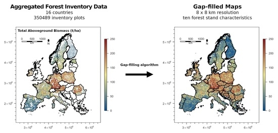
:Today, European forests face many challenges but also offer opportunities, such as climate change mitigation, provision of renewable resources, energy and other ecosystem services. Large-scale analyses to assess these opportunities are hindered by the lack of a consistent, spatial and accessible forest structure data. This study presents a freely available pan-European forest structure data set. Building on our previous work, we used data from six additional countries and consider now ten key forest stand variables. Harmonized inventory data from 16 European countries were used in combination with remote sensing data and a gap-filling algorithm to produce this consistent and comparable forest structure data set across European forests. We showed how land cover data can be used to scale inventory data to a higher resolution which in turn ensures a consistent data structure across sub-regional, country and European forest assessments. Cross validation and comparison with published country statistics of the Food and Agriculture Organization (FAO) indicate that the chosen methodology is able to produce robust and accurate forest structure data across Europe, even for areas where no inventory data were available.
1. Introduction
Since the pre-industrial period, the anthropogenic greenhouse gas emissions including carbon dioxide (CO2) have steadily increased and will have important impacts on human and natural systems [1]. Forests play an important role within the global carbon cycle because they store a large amount of carbon and mitigate climate change affects [2]. The reduction of greenhouse gas emissions by replacing fossil material and energy with renewable resources, such as biomass, is important to avoid the further increase in atmospheric CO2 concentration. Thus, the use of wood products is expected to increase since wood is important for a bio-based economy, aiming for a reduction in emissions from the combustion of fossil fuels. In addition, forests provide other important valuable ecosystem services such as the protection of infrastructure in mountainous areas, habitat for wildlife and recreation areas especially near large cities [3].
Forest ecosystems mitigate climate change effects, but they are also directly affected by climate change through changing growing conditions (e.g., temperature, precipitation and length of drought periods). Forest adaptation to changing environmental conditions takes time due to the long lifespan of trees [4,5]. Climate change is often associated with an increase in weather extremes such as drought or storm events followed by wildfires, wind throw and bark beetle infections [6,7]. This is an additional challenge to the forestry sector because the demanded ecosystem services need to be provided and secured for the future [8,9].
European forests cover about 33% of Europe’s total land area [3] and extend from the Mediterranean in the south to the Boreal regions in the north. They grow in elevations from sea level to high mountainous areas. These differences in the regional growing conditions have led to distinct ecosystems which are additionally shaped by the long-lasting historic management history in Europe [10]. Therefore, climate change, as an additional driver for forests, will also have distinct regional affects due to the geomorphological and climatic conditions [11,12,13]. Forest ecosystems and the belonging tree species are characterized by their eco-physiological heritage plus their land management history, both important for the adaptation potential of forest ecosystems [14,15].
Assessing the mitigation and adaptation potential of European forests requires consistent forest data across Europe. Such information may come from national forest reports or the Global Forest Resource Assessment (FRA) published by the United Nations Food and Agricultural Organization (FAO). These reports are often based on forest inventory data [16,17,18].
In Europe, National Forest Inventories (NFI) are commonly used to provide information for forest ecosystem service assessments [17]. However, it is important to note that the forest inventory monitoring system differs by country which leads to difficulties in comparing the results across countries and within Europe [19,20] since no consistent data collection system across Europe is in place. Each country has its own forest inventory system with its own methodology ranging from gridded sampling designs to forest surveys and/or a combination of remote sensing data with terrestrial forest information [17]. The FAO had some success in harmonizing definitions for their reports; however, only country totals such as aboveground biomass or deadwood are published [3,16]. Efforts to harmonize the different inventory systems or even establish a consistent forest monitoring system across Europe have proven to be a challenge [17,20,21,22,23].
The European Forest Information Scenario Model (EFIScen) uses and provides a freely available database for 32 European countries based on aggregated data at the county level [24]. These data are derived from information provided by the National Forest Inventories from each country and grouped by “forest types”. Since the size of the counties differ, the spatial boundaries are unknown, and the level of detail may vary between countries. Various gridded datasets were generated using the EFIScen data [25,26,27]. However, they only provide a limited set of forest attributes.
In response to the need for consistent spatial forest data across Europe, Moreno et al. [28] developed the first freely accessible pan-European spatially explicit gridded forest structure dataset using forest inventory data from countries with a systematic NFI system, that allowed data access. To our knowledge, few countries in Europe have no systematic plot-based forest inventory (such as Hungary, Bulgaria and Lithuania), some countries have a combination of satellite and terrestrial driven forest inventory (e.g., Italy) and the majority of countries have a systematic gridded permanent plot-level NFI in place. Moreno et al. [28] applied a gap-filling algorithm using remotely sensed net primary production (NPP), canopy height and climate data to produce a consistent gridded forest structure data set across Europe which allows analysis by countries, climatic and/or any other regional gradients. The data have been used for improving climate-sensitive models [29,30], for assessing climate limitations on forest structure and the mitigation potential of European forests [31,32]. Furthermore the data have been used for studies on the impact of conservation policies [33] and for quantifying the live tree carbon threatened by invasive alien pests [34].
The goal of this paper is to provide an improved version of this gridded forest structure data using the methodology of [28]. Based on the experiences of working with the previous data set, we added additional forest inventory data from four countries and for two regions previously not covered, included additional plot-level forest structure variables and further improved the resolution and the accuracy of this spatial forest data set. The objectives of our study are:
- to provide an improved gridded forest structure data set on 8 × 8 km resolution across Europe,
- to assess the error components of the new forest structure data,
- to obtain land cover information to generate consistent gridded forest structure maps at 500 m resolution enabling upscaling to regions and/or countries, and
- to evaluate the provided higher resolution maps by calculating country totals and compare these data to the original NFI data and the FAO statistics.
2. Materials and Methods
The principal approach of our study is to only use point sampled National Forest Inventory (NFI) data covering 16 different countries and apply a gap-filling algorithm for countries and regions where no such data are available. The R statistical software is used for data preparation, statistical analysis and data visualization [35]. The gap-filling is done using the Python script written and made publicly available by Moreno et al. [28]. Figure 1 provides the workflow and the used data including the methodological steps:
2.1. National Forest Inventory Data
The National Forest Inventory (NFI) data are obtained from 16 European countries and consist of recorded tree information from 350.489 inventory plots (Table 1). All selected countries maintain a gridded systematic point sampling National Forest Inventory. Data for 12 countries were available from a previous study by Moreno et al. [28] with additional details available in [36]. Data from the Czech Republic, used by Moreno et al. [28] were not used in our study. We obtained data from four additional countries, Albania, Croatia [37], Ireland [38] and the Netherlands [39]. We complemented the data from Italy [40,41] (now covering the whole country) and Belgium (now including also the region Wallonie). Overall, about 90.000 additional plot data were gathered. Each country has its own inventory system and sampling design (see Table 1) and use their own definitions and methods. All countries provided plot-level data based on their inventory system. The data were gathered, processed and harmonized as described in Neumann et al. [36]. Harmonization was done according to tree species groups, age classes and as far as possible for biomass and volume definitions (for details see [19,36]). However, basic definitions of volumes (e.g., inclusion of branches or measuring over or under bark) and sampling designs (e.g., diameter thresholds) cannot be changed which makes harmonization difficult [20,21,22]. The resulting data comprise a full set of plot-level forest variables derived from the recorded tree information on each plot and cover information such as the carbon content, biomass for individual compartments (stem, branch, foliage, root), volume, height, diameter at breast height, stem number, basal area, stand density index, age class and the tree species group. In the previous study [28], only six variables (carbon for whole tree, volume, basal area, diameter at breast height, height, age) were considered, while we extend the forest stand characteristics data to ten variables.
The plot-level inventory data are aggregated to 8 × 8 km grid by averaging the metric variables. For the nominal values (age class and tree species group), we calculate the proportion and most frequent value within an 8 × 8 km grid-cell based on the number of inventory points belonging to each class or group. At 8 × 8 km resolution, on average eight inventory plots are within a cell to ensure statistical confidence in the cell values [42]. It is important to note that Moreno et al. [28] used 0.133 × 0.133 degree resolution and WGS84 projection leading to a varying cell size from approximately 111 × 89 km at 37° latitude (e.g., southern Spain) to 111 × 43.5 km at 67° latitude (e.g., northern Finland). In this study, we use the ETRS89-LAEA projection with a fixed cell size of 8 × 8 km across latitude, providing consistent cell size and resolution in the whole study area (Figure 2).
2.2. Land Cover and Bioregions for Clustering
Following Moreno et al. [28], we use a bioregion map with six different regions: (i) Alpine, (ii) Atlantic, (iii) Boreal (including Boreal, Arctic and Norwegian Alpine), (iv) Continental (including Continental, Black Sea and Steppe), (v) Mediterranean and (vi) Pannonia. For land cover information, we use version 6 of the MODIS MCD12Q1 product with the University of Maryland (UMD) classification [44] representing land cover conditions of 2005. Spatial aggregation from 500 m to the 8 km resolution was needed to determine the most frequent land cover type within the 8 km grid cell. Only cells dominated by a vegetation land cover type are used for the gap-filling, while cells that are dominated by urban and other non-vegetated land are excluded.
2.3. Co-Variates for Gap-Filling
We use the following variables as co-variates in the gap-filling algorithm: Net primary production, net primary production trend, canopy height and a climate limitation index.
Net Primary Production (NPP) at 0.0083° resolution is derived using the original MOD17 algorithm for global calculations in combination with a European climate dataset which has improved the NPP estimations for European forests [45,46]. For net primary production trend, a linear regression line is fitted to the annual NPP values of 2000 to 2012 at the original 0.0083° resolution. The trend is given by the slope of the regression line.
Tree canopy height is obtained from a global spaceborne lidar data forest canopy height map at 0.0083° resolution [47]. The climate limitation index is the product of three normalized climate datasets: relative growing season length, average annual short-wave solar radiation and average annual vapor pressure deficit. Average growing season length is estimated by using the average time between the onset of the increasing leaf area index (LAI) in spring and the end of the decreasing LAI in autumn using the MODIS Leaf Area Index data [48]. Both short-wave solar radiation and vapor pressure deficit are calculated using the MtClim algorithm which uses climate data and a digital elevation model as inputs [46,49]. Therefore, by using the climate limitation index the elevational gradient is also considered. The climate limitation index was still available from the previous work carried out by Moreno et al. [28]. All data are aggregated to 8 km resolution by calculating the average value within the cell.
2.4. K-Means Clustering and k-Nearest Neighbor Gap-Filling
We apply the landcover and bioregion data and the above-mentioned co-variates in a two-step gap-filling algorithm which (i) clusters cells by similarity and (ii) uses a k-Nearest Neighbor algorithm to fill empty cells. In step number one, cells are grouped according to their land cover and related biogeographical region using a k-means clustering algorithm for assigning all grid cells to their corresponding cluster. In step number two, each cell with missing gridded inventory data is assigned to its nearest neighbor with inventory data belonging to the same cluster using a k-Nearest Neighbor (kNN) algorithm. The kNN method is a non-parametric approach used to predict the values of variables by finding the k most similar objects with observed values within a user-defined co-variate space [49]. Similarity is based on the (Euclidean) distance between the objects in the co-variate space [50]. Following Moreno et al. [28], two k-means cluster and one nearest neighbor are applied. Thus, each cell without NFI data is provided with NFI data from the cell which (i) has NFI data, (ii) belongs to the same cluster as the cell with missing data and (iii) is from all cells fulfilling these two conditions, its nearest neighbor in the co-variate space formed by NPP, NPP trend, canopy height and climate limitation index.
2.5. Forest Area Mask
We use the MODIS land cover data and UMD classification to produce a forest area mask at 500 × 500 m resolution. The UMD land cover classification is among other things based on tree cover and canopy height. We use this information to assign a forest area to a land cover class. Each forest land cover class, (i) Evergreen Needleleaf, (ii) Evergreen Broadleaf, (iii) Deciduous Needleleaf, (iv) Deciduous Broadleaf, (v) Mixed, are defined by a tree cover > 60% and a canopy height > 2 m. In our forest area mask, cells belonging to these classes are assumed to be fully forested and contribute 25 ha (500 m × 500 m) of forest area. Woody Savannas have by definition a tree coverage of 30%–60% and we therefore define a factor of 0.45 for calculating the forest area for such cells, meaning that each cell contributes 11.25 ha. For Savannas, we defined a factor of 0.15 (3.75 ha) and for Cropland/Natural Vegetation Mosaics a factor of 0.05 (1.25 ha) is used. All other land cover classes (e.g., Closed/Open Shrublands, Grasslands, Croplands) are assumed to be non-forested.
2.6. Calculation of Country Sums and Comparison with FAO Statistics
The forest area mask (ha) is combined with the gap-filled volume map (m3/ha) to produce a total volume (m3) map at 500 m resolution. The values of this map are summarized by country and compared with the mean volumes for the years 2000 to 2010 as reported in the State of Europe’s Forest 2015 (FAO) [3]. The period 2000 to 2010 is chosen as it best coincides with the inventory data we used for the gap-filling (Table 1). Linear regression is used to determine goodness-of-fit and bias of our estimations.
3. Results
3.1. An Improved Gridded Forest Structure Data
Even though the collected NFI data covers large forest areas in Europe, there are still regions where no systematic grid-sampled forest inventory data were available (see Figure 2). Another issue is the fact that due to differences in the data recording system and the grid raster by country, differences between countries may occur. The missing forest inventory information from countries where no data were available is filled with the two-step gap-filling algorithm by identifying for every cell where no forest inventory data are available, its most similar cell that does provide such data.
After applying the gap-filling algorithm, a full set of pan-European gridded data comprising volume, carbon content, biomass by compartment, height, diameter at breast height, stem number, basal area, stand density index, age class and tree species group is generated. Volume, carbon content, biomass, stem number and basal area given in per hectare values. All other variables represent the mean average characteristics by cell independent of the forest area of this cell. The results by cell for selected variables are given as maps in Figure 3, Figure 4, Figure 5 and Figure 6 and include grid-cells with low tree cover such as mixed forest-agriculture cells or small forests in urban areas.
3.2. Accuracy of the Improved Data Set
An important issue with data is its accuracy. Thus, we next assess the error range of the gap-filling algorithm by executing ‘leave-one-out’ and ‘country-wise’ cross validations. The ‘leave-one-out’ cross validation is performed by iteratively removing data from one cell and gap-fill this cell using the data of all other cells. The ‘country-wise’ cross validation is performed by iteratively removing the entire data from a country and filling all cells within that country only with data from all other countries. We calculate the mean value and the standard deviation (SD) of the gap-filled data sets as well as the mean bias error (MBE), the mean absolute error (MAE) and the root mean square error (RMSE). These measures are compared with the mean value, SD and confidence interval (CI, α = 0.05) of the original inventory data.
The mean and SD of the gap-filled data is nearly the same as in the original data in the case of the ‘leave-one-out’ cross validation and shows, depending on the variable considered, no or only little bias (Table 2). The ‘country-wise’ cross validation shows negative bias for all variables, leading to lower mean values, while the SD is slightly higher than, but still comparable to, the SD of the original data. MAE and RMSE are close to the CI for the ‘leave-one-out’ cross validation. The ‘country-wise’ cross validation shows higher values for the MAE and RMSE, with the MAE still being comparable to the SD.
At country level, the error is expressed as the median of the relative difference in percent between the aggregated inventory data versus the gap-filled data (see Table 3). Our results of the cross validation on the country level exhibit for the ‘country-wise’ cross validation a higher error than ‘leave-one-out.’ No pattern is evident, suggesting that regions, latitude or longitude, are associated with higher errors. At the EU level, the median of the percentage relative difference is close to zero for ‘leave-one-out’, while for the county vise validation it is around 10% and is evident for all produced variables except the most frequent age class (see Table 3).
3.3. Upscaling Data
An important part of this study is to deliver consistent European forest data across countries and regions at any spatial resolution. For the upscaling, we use the forest area mask derived from MODIS land cover data at a 500 × 500 m resolution. By combining the forest area mask with the 8 × 8 km gap-filled maps, we produce maps at 500 × 500 m resolution which better reflect the possible heterogeneity of the landscape within an 8 × 8 km grid cell (Figure 7, Figure 8 and Figure 9). An 8 × 8 km cell may only be partly forested and also contain urban areas, water bodies or agricultural land. These maps can then be used in combination with other data available at a similar resolution to study certain aspects of European forests, such as the legal or technical accessibility of forest resources.
3.4. Evaluate the Results Using FAO Statistics
Important for this study is comparing our derived information with other available data such as the State of Europe’s Forests (FAO) statistics [3], as this allows to assess the quality of the gap-filling algorithm in countries, where no NFI data were available. In general, a high agreement between our produced volume estimates versus the reported values (Adj R2 = 0.903) are evident (Figure 10 and Figure 11). When looking at the European scale, almost no bias (Slope = 0.964) is present. However, some countries (e.g., Bulgaria, France, Romania, Spain) do show substantial overestimation or underestimation (Figure 10 and Figure 11). When only looking at countries where no inventory information was available, there is also an overall good agreement (Adj R2 = 0.787) between our estimations and the reported values (Figure 11b). In this case, the estimates in general tend to be higher than the reported values (Slope = 1.12). Individual countries can be overestimated or underestimated, in some cases substantially (e.g., Bosnia-Herzegovina, Bulgaria, Serbia). Estimations are close to the reported values for some countries where we had inventory information (Austria, Belgium, Estonia, Finland, Italy, Netherlands, Poland) as well as countries without that information (Czech Republic, Greece, Hungary, Latvia, Montenegro, Slovenia, United Kingdom) (Figure 10 and Figure 11).
4. Discussion
Lack of a consistent and accessible European forest inventory data makes detailed analysis at the European level difficult or even impossible [17,19]. With this study, we provide and produce a pan-European gridded forest structure dataset based on an extensive collection of point sampled National Forest Inventory data, remote sensing information and a gap-filling algorithm for those areas where no gridded data were collected or gridded inventory data were not available. With these data, we are able to depict forest structure differences at the regional and sub-regional levels which allows detailed forest analysis across Europe (Figure 3, Figure 4, Figure 5 and Figure 6).
Cross validation is used to assess the quality and accuracy of the data. The results show that the chosen methodology is robust and accurate which gives confidence in the produced data. The gap-filling algorithm relies on the regional distribution of the input inventory data and how well it covers the latitudinal and elevational gradients, climatic conditions and bioregions in Europe. Only high coverage of the relevant conditions ensures that the nearest object determined by the kNN algorithm really bears similarity with the object which variable values need to be predicted. This limitation is evident when looking at the ‘country−wise’ cross validation results. When removing the entire data from a country where prevailing conditions (e.g., climatic, management history) are not well covered by the remaining data of all the other countries, the uncertainty tends to be higher. This can be observed for Spain on the Iberian Peninsula, Ireland on the British Isles, as well as Albania and Croatia in the north-eastern Mediterranean. This may also be evident for the Netherlands, where our produced inventory volume and DBH values are lower compared to the neighboring countries Belgium and Germany, which are likely to be used for gap-filling.
When removing data from an entire country and the growing conditions are well covered by the remaining data from the neighboring countries, the error tends to be lower, e.g., Austria, France or Germany. Being aware of these limitations, in this study we specifically added data from Albania, Croatia and Ireland to better cover these regions.
Differences in the sampling design or calculation method among countries, such as the minimum diameter at breast height required for a tree to be included or biomass function used, could also explain high errors. For instance, when removing the entire data from Sweden, it is likely that it will be filled with data coming from the two other Scandinavian countries. However, Sweden uses fixed area plots with no minimum diameter requirement, while Norway, although also using fixed area plots, requires trees to have a minimum diameter at breast height of 5 cm and Finland uses angle count sampling, which is a different plot design altogether.
4.1. Comparison with FAO Statistics
Comparison with FAO statistics gives further confidence in the chosen methodology and produced data, especially on the European scale where agreement between calculated and reported values is high. This high agreement was expected when only looking at countries were we did gather inventory data, as also the FAO statistics are mainly based on national inventories [18]. However, for some of these countries substantial overestimation or underestimation can still be observed. The reasons can be manifold.
In Romania, reported growing stock for the years 2000, 2005 and 2010 are estimated using a relationship between forest area and a mean growing stock by unit of area based on the Forest Inventory in 1985, while the estimation for 2015 is based on the National Forest Inventory 2012, the same inventory our data for Romania comes from. The growing stock reported for 2015 is substantially higher than the previous reported values (2222 million m3 in 2015 versus 1378 million m3 in 2010) and closer to our estimations [51]. However, in our study, we only compare with the mean of the values reported for the period 2000 to 2010, as this period overall coincides best with our gathered inventory data. In general, different time periods can affect the comparison as we considered the mean of the reported values for the period 2000 to 2010 for all countries, although the inventory data in individual countries do not cover this whole period (Table 1).
In Sweden, a different minimum diameter requirement for trees to be considered between FAO report (minimum of 10 cm) and NFI data (no minimum requirement) may contribute to overestimation [52]. In general, problems with the harmonization of variables and definitions such as stem volume [22], growing stock [20], forest available for wood supply or even forest in general [18,21] could partly explain some of the observed differences.
These differences in the definitions of forest and forest available for wood supply lead to different forest area estimations which can be another reason for overestimation or underestimation [53]. The FAO defines forest as, “land spanning more than 0.5 ha with trees higher than 5 m and a canopy cover of more than 10%, or trees able to reach these thresholds in situ. It does not include land that is predominantly under agricultural or urban land use” [54]. In addition to the presence of trees the definition is also land-use based, meaning that temporarily unstocked areas intended for forestry or conservation use are included [54,55]. In our study, a forest area mask is generated using MODIS land cover data, which relies on the presence or absence of tree cover to identify forests and cannot account for intended land use [55]. The coarse resolution of 500 × 500 m (25 ha) also means that not only the Forest or Woody Savanna land cover types contain forest as basically every cell irrespective of the land cover class can contain forest as defined by the FAO, i.e., a land spanning more than 0.5 ha with trees higher than 5 meters and a canopy cover of more than 10%. We partly considered this in our forest area mask by assuming all Forest land cover cells to be fully forested, compensating for small forest areas in cells with land cover classes which did not contribute to forest area in our study. We also introduced forest area factors for selected other land cover classes, such as Woody Savannas, Savannas or Cropland/Natural Vegetation Mosaic. Differences between reported global forest cover change in the Global Forest Resources Assessment 2015 (FRA 2015) and global remote sensing estimations by Hansen et al. [56,57] could also possibly be explained by the used tree cover threshold of 25% and also by the coarse resolution of the MODIS images used in the earlier of the two studies [55]. We also explored the usage of the high-resolution 25 × 25 m CORINE land cover data to estimate forest area (Appendix A) [58]. Underestimation of forest area might be the main reason for the substantial underestimation of volume in France and Spain. In both countries, the share of 500 m cells belonging to one of the Forest MODIS land cover classes are low compared to other countries. As savannas and shrublands cover large areas in these countries, our approach may be unable to account for all the small forest areas in cells belonging to these and other classes. This could be improved by using a different approach based on forest cover data or using different land cover data such as CORINE [59,60]. However, detailed analysis of all possible reasons for overestimating or underestimating and optimizing our estimations were not the aim and scope of our study. Furthermore, when using the gap-filled data, one is not limited to the forest area mask proposed in this study but can use any other forest area mask.
In countries where no inventory data were obtained, overestimation or underestimation can, in addition to the reasons already mentioned, also be related to the inventory data not covering the prevalent conditions in these countries well enough (see also Section 4.1). In south-east Europe, we were only able to gather data from Albania and Croatia, which might not be sufficient to accurately describe the situation in other countries belonging to this region, as suggested by the observed overestimation in many of these countries (Bosnia and Herzegovina (BA), Bulgaria (BG), Greece (EL), the Republic of North Macedonia (MK) and Serbia (RS)). As a consequence, although we were able to add the data from Albania and Croatia for this study, additional data from that region are likely needed to improve the forest structure data.
4.2. Potential Applications
A big advantage of high-quality spatial explicit gridded forest structure data is the ability to combine it with other spatial explicit information, such as soil information, conservation status, land cover, climate data or terrain data. This allows for detailed analysis which can contribute to solving and providing relevant questions related to the carbon mitigation potential of European forests, the impact of conservation policies or how forest resources are threatened by changing disturbance regimes [31,32,33,34]. A most recent example is the assessment of the harvestable forest area and stocking volume in Europe [61]. The study combines the Forest Structure data with conservation status, slope, soil and road infrastructure data to quantify the legal and technical accessibility of forest resources for mechanized harvesting. The availability of wood resources is an important question in regard to the potential of using wood products to substitute non−renewable fossil products. Another application is initializing large-scale, climate-sensitive bio-geochemical-mechanistic forest simulation models. All these studies can support decision makers during the transition towards a bio-based economy.
4.3. Room for Improvement
The lack of a common inventory system across European forests with standardized definitions as well as sampling designs and measurement methods, make a comparison of even basic forest variables, such as forest area or growing stock difficult in Europe. Our harmonization of the different national forest inventory data with the improved data sources and methodology is important part for consistent pan-European forest studies. If a common inventory system as well as a common forest area mask could be established, the methods described in this study could be used to support countries in official reporting of key forest variables. The results of this study are an important attempt to provide consistent forest structure data to the scientific community.
Author Contributions
Conceptualization, C.P. and H.H.; methodology, C.P.; software, C.P.; validation, C.P.; formal analysis, C.P.; investigation, C.P. and M.N.; resources, C.P.; data curation, C.P. and M.N.; writing—original draft preparation, C.P. writing—review and editing, M.N. and H.H.; visualization, C.P.; supervision, H.H.; project administration, H.H.; funding acquisition, H.H. All authors have read and agreed to the published version of the manuscript.
Funding
This work was supported by the Bio-Based Industries Joint Undertaking under the European Union’s Horizon 2020 research and innovation program, TECH4EFFECT—Techniques and Technologies or Effective Wood Procurement project [Grant Number 720757]. Additional financial support came from the «GIS and Remote Sensing for Sustainable Forestry and Ecology (SUFOGIS)» project funded with support from the EU ERASMUS+ program. The European Commission support for the production of this publication does not constitute an endorsement of the contents, which reflects the views only of the authors, and the Commission cannot be held responsible for any use which may be made of the information contained therein.
Data Availability Statement
The produced forest structure data set are (will be) openly available at: ftp://palantir.boku.ac.at/Public/ImprovedForestCharacteristics/ (accessed on 30 November 2021).
Acknowledgments
We acknowledge the open data policies by European forest inventory agencies, that made this analysis possible. Parts of the used inventory data were gathered as part of the collaborative project ‘FORest management strategies to enhance the MITigation potential of European forests’ (FORMIT), which received funding from the European Union Seventh Framework Programme under grant agreement n° 311970. We would like to thank John Redmond and Luke Heffernan and the Department of Agriculture, Food and the Marine for providing national forest inventory data for Ireland. The data used for Ireland are the property of the Department of Agriculture, Food and the Marine, Ireland. We appreciate the help of Huguez Lecomte and Andre Thibaut (Service Public de Wallonie) and Sebastien Bauwens (University of Liege) for their support with the Wallonian forest inventory. The data used for Wallonia are the property of SPW−DGARNE. We thank Elvin Toromani (University of Tirana) for his support analyzing the Albanian forest inventory. We further extend our gratitude to Jura Cavlovic (University of Zagreb, Croatia) and Goran Videc (Ministry of Agriculture, Croatia) for their support with the Croatian forest inventory. The data used for Croatia are the property of the Croatian Ministry of Agriculture. We acknowledge the open access to national forest inventory data from Italy and Netherlands.
Conflicts of Interest
The authors declare no conflict of interest.
Appendix A
During the course of our study, we also explored the usage of CORINE land cover data for the production of the forest area mask. The higher resolution 25 × 25 m data is better able to detect small forested areas which might be overlooked when using the coarse 500 × 500 m MODIS land cover data (see Section 4.1). For the CORINE forest area mask, each cell belonging to a Forest land cover class contributed 0.0625 ha (25 × 25 m) of forest area, while cells belonging to other land cover classes did not contribute any forest area.
In some countries such as Finland, France, Norway or Spain, difference in estimated forest area is substantial, while in other countries (e.g., Austria, Bulgaria, Romania) the difference is only minor (Figure A1). Especially in France and Spain, the forest area estimated with the CORINE data is likely way closer to the true value compared to the estimations based on the MODIS data. However, although overall the model estimations better fitted the reported values (Figure A2a), this was not true when only looking at countries where we did not have inventory data (Figure A2b). Therefore, we decided to still use the MODIS land cover data for forest area estimation as this data set are already used in the gap-filling algorithm. It is important to stress that the gap-filled maps can be combined with any other forest area mask and using forest area mask with higher resolution is encouraged. In this study, we simply provide one way of creating a forest area mask using MODIS land cover data, which was sufficient for our needs. It was not the aim of the study to provide the best possible forest area mask.
Figure A1.
Comparison of the forest area estimations based on MODIS [44] and CORINE [58] land cover data sets. MODIS refers to the forest area mask as used in this study (see Section 2.5) while CORINE refers to a forest area mask based on CORINE land cover data which was not used in the study (see Appendix A). Countries where no inventory data were available are marked with an asterisk.

Figure A2.
Comparison of the volume calculated from our Forest Structure Data versus the mean of the volumes for the period 2000 to 2010 as reported in State of Europe’s Forest 2015 [3] (Ind 1.2B Change in growing stock on forests). Forest Structure Data refers to the values calculated by combining the gap-filled maps with land cover information to calculate country totals (see Figure 7). In this case, underlying forest area estimations are based on CORINE land cover data, compared to Figure 11 where forest area estimations are based an MODIS land cover data as used in the study. Linear regression results R² (Adj R²), Intercept, Slope and p−Value (P) are shown. (a) Shows results when using all countries, irrespective if National Forest Inventory (NFI) data were available. (b) Shows the results only for countries where no NFI data were available. Country codes are: AL = Albania, AT = Austria, BA = Bosnia−Herzegovina*, BE = Belgium, BG = Bulgaria*, CZ = Czech Republic*, CH = Switzerland*, DE = Germany, DK = Denmark*, EE = Estonia, EL = Greece*, ES = Spain, FI = Finland, FR = France, HR = Croatia, HU = Hungary*, IE = Ireland, IT = Italy, LT = Lithuania*, LU = Luxemburg*, LV = Latvia*, ME = Montenegro*, MK = North Macedonia*, NL = Netherlands, NO = Norway, PL = Poland, PT = Portugal*, RO = Romania, RS = Serbia*, SE = Sweden, SI = Slovenia*, SK = Slovakia*, UK = United Kingdom*; Countries where no inventory data were present are marked with an asterisk.

References
- IPCC. Climate Change 2014: Synthesis Report. Contribution of Working Groups I, II and III to the Fifth Assessment Report of the Intergovernmental Panel on Climate Change; Core Writing Team, Pachauri, R.K., Meyer, L.A., Eds.; IPCC: Geneva, Switzerland, 2014; ISBN 9789291691432. [Google Scholar]
- Pan, Y.; Birdsey, R.A.; Fang, J.; Houghton, R.; Kauppi, P.E.; Kurz, W.A.; Phillips, O.L.; Shvidenko, A.; Lewis, S.L.; Canadell, J.G.; et al. A large and persistent carbon sink in the world’s forests. Science 2011, 333, 988–993. [Google Scholar] [CrossRef] [Green Version]
- Forest Europe. State of Europe’s Forests 2015; Forest Europe: Madrid, Spain, 2015. [Google Scholar]
- Lindner, M.; Maroschek, M.; Netherer, S.; Kremer, A.; Barbati, A.; Garcia-Gonzalo, J.; Seidl, R.; Delzon, S.; Corona, P.; Kolström, M.; et al. Climate change impacts, adaptive capacity, and vulnerability of European forest ecosystems. For. Ecol. Manag. 2010, 259, 698–709. [Google Scholar] [CrossRef]
- Lindner, M.; Fitzgerald, J.B.; Zimmermann, N.E.; Reyer, C.; Delzon, S.; van der Maaten, E.; Schelhaas, M.J.; Lasch, P.; Eggers, J.; van der Maaten-Theunissen, M.; et al. Climate change and European forests: What do we know, what are the uncertainties, and what are the implications for forest management? J. Environ. Manag. 2014, 146, 69–83. [Google Scholar] [CrossRef] [Green Version]
- Senf, C.; Pflugmacher, D.; Zhiqiang, Y.; Sebald, J.; Knorn, J.; Neumann, M.; Hostert, P.; Seidl, R. Canopy mortality has doubled in Europe’s temperate forests over the last three decades. Nat. Commun. 2018, 9, 4978. [Google Scholar] [CrossRef] [PubMed]
- Seidl, R.; Schelhaas, M.J.; Rammer, W.; Verkerk, P.J. Increasing forest disturbances in Europe and their impact on carbon storage. Nat. Clim. Chang. 2014, 4, 806–810. [Google Scholar] [CrossRef] [PubMed] [Green Version]
- Dyderski, M.K.; Paź, S.; Frelich, L.E.; Jagodziński, A.M. How much does climate change threaten European forest tree species distributions? Glob. Chang. Biol. 2018, 24, 1150–1163. [Google Scholar] [CrossRef] [PubMed]
- Hanewinkel, M.; Cullmann, D.A.; Schelhaas, M.-J.; Nabuurs, G.-J.; Zimmermann, N.E. Climate change may cause severe loss in the economic value of European forest land. Nat. Clim. Chang. 2013, 3, 203–207. [Google Scholar] [CrossRef]
- McGrath, M.J.; Luyssaert, S.; Meyfroidt, P.; Kaplan, J.O.; Bürgi, M.; Chen, Y.; Erb, K.; Gimmi, U.; McInerney, D.; Naudts, K.; et al. Reconstructing European forest management from 1600 to 2010. Biogeosciences 2015, 12, 4291–4316. [Google Scholar] [CrossRef] [Green Version]
- Anderson-Teixeira, K.J.; Herrmann, V.; Rollinson, C.R.; Gonzalez, B.; Gonzalez-Akre, E.B.; Pederson, N.; Alexander, M.R.; Allen, C.D.; Alfaro-Sánchez, R.; Awada, T.; et al. Joint effects of climate, tree size, and year on annual tree growth derived from tree-ring records of ten globally distributed forests. Glob. Chang. Biol. 2022, 28, 245–266. [Google Scholar] [CrossRef] [PubMed]
- Latte, N.; Perin, J.; Kint, V.; Lebourgeois, F.; Claessens, H. ajor changes in growth rate and growth variability of beech (Fagus sylvatica L.) related to soil alteration and climate change in Belgium. Forests 2016, 7, 174. [Google Scholar] [CrossRef] [Green Version]
- Pretzsch, H.; Biber, P.; Schütze, G.; Uhl, E.; Rötzer, T. Forest stand growth dynamics in Central Europe have accelerated since 1870. Nat. Commun. 2014, 5, 4967. [Google Scholar] [CrossRef] [PubMed] [Green Version]
- Kulakowski, D.; Seidl, R.; Holeksa, J.; Kuuluvainen, T.; Nagel, T.A.; Panayotov, M.; Svoboda, M.; Thorn, S.; Vacchiano, G.; Whitlock, C.; et al. A walk on the wild side: Disturbance dynamics and the conservation and management of European mountain forest ecosystems. For. Ecol. Manag. 2017, 388, 120–131. [Google Scholar] [CrossRef] [PubMed] [Green Version]
- Kolström, M.; Lindner, M.; Vilén, T.; Maroschek, M.; Seidl, R.; Lexer, M.J.; Netherer, S.; Kremer, A.; Delzon, S.; Barbati, A.; et al. Reviewing the science and implementation of climate change adaptation measures in European forestry. Forests 2011, 2, 961–982. [Google Scholar] [CrossRef] [Green Version]
- FAO. Global Forest Resources Assessment 2015; Elsevier B.V.: Rome, Italy, 2015; ISBN 978-92-5-108826-5. [Google Scholar]
- Tomppo, E.; Gschwantner, T.; Lawrence, M.; McRoberts, R.E. (Eds.) National Forest Inventories; Springer: Dordrecht, The Netherlands, 2010; ISBN 978-90-481-3232-4. [Google Scholar]
- Vidal, C.; Alberdi, I.; Redmond, J.; Vestman, M.; Lanz, A.; Schadauer, K. The role of European National Forest Inventories for international forestry reporting. Ann. For. Sci. 2016, 73, 793–806. [Google Scholar] [CrossRef] [Green Version]
- Neumann, M.; Moreno, A.; Mues, V.; Härkönen, S.; Mura, M.; Bouriaud, O.; Lang, M.; Achten, W.M.J.; Thivolle-Cazat, A.; Bronisz, K.; et al. Comparison of carbon estimation methods for European forests. For. Ecol. Manag. 2016, 361, 397–420. [Google Scholar] [CrossRef]
- Gschwantner, T.; Alberdi, I.; Bauwens, S.; Bender, S.; Borota, D.; Bosela, M.; Bouriaud, O.; Breidenbach, J.; Donis, J.; Fischer, C.; et al. Growing stock monitoring by European National Forest Inventories: Historical origins, current methods and harmonisation. For. Ecol. Manag. 2022, 505, 119868. [Google Scholar] [CrossRef]
- Vidal, C.; Lanz, A.; Tomppo, E.; Schadauer, K.; Gschwantner, T.; Di Cosmo, L.; Robert, N. Establishing forest inventory reference definitions for forest and growing stock: A study towards common reporting. Silva Fenn. 2008, 42, 247–266. [Google Scholar] [CrossRef] [Green Version]
- Gschwantner, T.; Alberdi, I.; Balázs, A.; Bauwens, S.; Bender, S.; Borota, D.; Bosela, M.; Bouriaud, O.; Donis, J.; Gschwantner, T.; et al. Harmonisation of stem volume estimates in European National Forest Inventories. Ann. For. Sci. 2019, 76, 24. [Google Scholar] [CrossRef] [Green Version]
- Tomppo, E.O.; Schadauer, K. Harmonization of national forest inventories in Europe: Advances under Cost Action E43. For. Sci. 2012, 58, 191–200. [Google Scholar] [CrossRef]
- Schelhaas, M.J.; Varis, S.; Schuck, A.; Nabuurs, G.J. EFISCEN Inventory Database; European Forest Institute: Joensuu, Finland, 2006. [Google Scholar]
- Vilén, T.; Gunia, K.; Verkerk, P.J.; Seidl, R.; Schelhaas, M.J.; Lindner, M.; Bellassen, V. Reconstructed forest age structure in Europe 1950–2010. For. Ecol. Manag. 2012, 286, 203–218. [Google Scholar] [CrossRef]
- Gallaun, H.; Zanchi, G.; Nabuurs, G.J.; Hengeveld, G.; Schardt, M.; Verkerk, P.J. EU-wide maps of growing stock and above-ground biomass in forests based on remote sensing and field measurements. For. Ecol. Manag. 2010, 260, 252–261. [Google Scholar] [CrossRef]
- Verkerk, P.J.; Fitzgerald, J.B.; Datta, P.; Dees, M.; Hengeveld, G.M.; Lindner, M.; Zudin, S. Spatial distribution of the potential forest biomass availability in europe. For. Ecosyst. 2019, 6, 5. [Google Scholar] [CrossRef]
- Moreno, A.; Neumann, M.; Hasenauer, H. Forest structures across Europe. Geosci. Data J. 2017, 4, 17–28. [Google Scholar] [CrossRef]
- Härkönen, S.; Neumann, M.; Mues, V.; Berninger, F.; Bronisz, K.; Cardellini, G.; Chirici, G.; Hasenauer, H.; Koehl, M.; Lang, M.; et al. A climate-sensitive forest model for assessing impacts of forest management in Europe. Environ. Model. Softw. 2019, 115, 128–143. [Google Scholar] [CrossRef]
- Neumann, M.; Godbold, D.L.; Hirano, Y.; Finér, L. Improving models of fine root carbon stocks and fluxes in European forests. J. Ecol. 2020, 108, 496–514. [Google Scholar] [CrossRef] [Green Version]
- Hasenauer, H.; Neumann, M.; Moreno, A.; Running, S. Assessing the resources and mitigation potential of European forests. Energy Procedia 2017, 125, 372–378. [Google Scholar] [CrossRef]
- Moreno, A.; Neumann, M.; Hasenauer, H. Climate limits on European forest structure across space and time. Glob. Planet. Chang. 2018, 169, 168–178. [Google Scholar] [CrossRef]
- Moreno, A.; Neumann, M.; Mohebalian, P.M.; Thurnher, C.; Hasenauer, H. The Continental Impact of European Forest Conservation Policy and Management on Productivity Stability. Remote Sens. 2019, 11, 87. [Google Scholar] [CrossRef] [Green Version]
- Seidl, R.; Klonner, G.; Rammer, W.; Essl, F.; Moreno, A.; Neumann, M.; Dullinger, S. Invasive alien pests threaten the carbon stored in Europe’s forests. Nat. Commun. 2018, 9, 1626. [Google Scholar] [CrossRef]
- R Core Team. R: A Language and Environment for Statistical Computing; R Foundation for Statistical Computing: Vienna, Austria, 2020. [Google Scholar]
- Neumann, M.; Moreno, A.; Thurnher, C.; Mues, V.; Härkönen, S.; Mura, M.; Bouriaud, O.; Lang, M.; Cardellini, G.; Thivolle-Cazat, A.; et al. Creating a regional MODIS satellite-driven net primary production dataset for european forests. Remote Sens. 2016, 8, 554. [Google Scholar] [CrossRef] [Green Version]
- Vidal, C.; Alberdi, I.A.; Hernández Mateo, L.; Redmond, J.J. (Eds.) National Forest Inventories; Springer International Publishing: Cham, Switzerland, 2016; ISBN 978-3-319-44014-9. [Google Scholar]
- Department of Agriculture, Food and the Marine. Ireland’s National Forest Inventory 2017 Field Procedures and Methodology; Department of Agriculture, Food and the Marine: Dublin, Ireland, 2017; ISBN 9781406429800. [Google Scholar]
- Schelhaas, M.J.; Clerkx, A.P.P.M.; Daamen, W.P.; Oldenburger, J.F.; Velema, G.; Schnitger, P.; Schoonderwoerd, H.; Kramer, H. Zesde Nederlandse Bosinventarisatie: Methoden en Basisresultaten; Alterra-Rapport 2545; Alterra Wageningen UR (University & Research Centre): Wageningen, The Netherlands, 2014. [Google Scholar]
- Gasparini, P.; Tabacchi, G. L’Inventario Nazionale delle Foreste e dei serbatoi forestali di Carbonio INFC 2005. In Secondo inventario forestale nazionale italiano. Metodi e risultati. Ministero delle Politiche Agricole, Alimentari e Forestali; Corpo Forestale dello Stato; Consiglio per la Ricerca e la Sperimentazione in Agricoltura, Unità di ricerca per il Monitoraggio e la Pianificazione Forestale, Edagricole: Milano, Italy, 2011; p. 650. Available online: https://shop.newbusinessmedia.it/collections/edagricole/products/l-inventario-nazionale-delle-foreste-e-dei-serbatoi-forestali-di (accessed on 30 November 2021).
- Gasparini, P.; Di Cosmo, L.; Floris, A.; Notarangelo, G.; Rizzo, M.; Guida per i Rilievi in Campo. INFC2015—Terzo Inventario Forestale Nazionale. Consiglio per la Ricerca in Agricoltura e L’analisi Dell’economia Agraria, Unità di Ricerca per il Monitoraggio e la Pianificazione Forestale (CREA-MPF); Corpo Forestale dello Stato, Ministero per le Politiche Agricole, Alimentari e Forestali: Agordo, Italy, 2016; ISBN 9788899595449. Available online: https://www.inventarioforestale.org/it/node/82 (accessed on 30 November 2021).
- Moreno, A.; Neumann, M.; Hasenauer, H. Optimal resolution for linking remotely sensed and forest inventory data in Europe. Remote Sens. Environ. 2016, 183, 109–119. [Google Scholar] [CrossRef]
- Hasenauer, H.; Eastaugh, C.S. Assessing Forest Production Using Terrestrial Monitoring Data. Int. J. For. Res. 2012, 2012, 961576. [Google Scholar] [CrossRef] [Green Version]
- Friedl, M.; Sulla-Menashe, D. MCD12Q1 MODIS/Terra+Aqua Land Cover Type Yearly L3 Global 500 m SIN Grid V006 [Data set]. NASA EOSDIS Land Processes DAAC. 2019. Available online: https://ladsweb.modaps.eosdis.nasa.gov/missions-and-measurements/products/MCD12Q1/#data-availability (accessed on 4 September 2019).
- Running, S.W.; Nemani, R.R.; Heinsch, F.A.; Zhao, M.; Reeves, M.; Hashimoto, H. A Continuous Satellite-Derived Measure of Global Terrestrial Primary Production. Bioscience 2004, 54, 547–560. [Google Scholar] [CrossRef]
- Moreno, A.; Hasenauer, H. Spatial downscaling of European climate data. Int. J. Climatol. 2015, 36, 1444–1458. [Google Scholar] [CrossRef]
- Simard, M.; Pinto, N.; Fisher, J.B.; Baccini, A. Mapping forest canopy height globally with spaceborne lidar. J. Geophys. Res. Biogeosci. 2011, 116, 1–12. [Google Scholar] [CrossRef] [Green Version]
- Myneni, R.B.; Hoffman, S.; Knyazikhin, Y.; Privette, J.L.; Glassy, J.; Tian, Y.; Wang, Y.; Song, X.; Zhang, Y.; Smith, G.R.; et al. Global products of vegetation leaf area and fraction absorbed PAR from year one of MODIS data. Remote Sens. Environ. 2002, 83, 214–231. [Google Scholar] [CrossRef] [Green Version]
- McRoberts, R.E.; Nelson, M.D.; Wendt, D.G. Stratified estimation of forest area using satellite imagery, inventory data, and the k-Nearest Neighbors technique. Remote Sens. Environ. 2002, 82, 457–468. [Google Scholar] [CrossRef]
- Manning, C.D.; Schütze, H. Foundations of Statistical Natural Language Processing. SIGMOD Rec. 2002, 31, 37–38. [Google Scholar] [CrossRef]
- FAO. Global Forest Resources Assessment 2015 Country Report Romania; FAO: Rome, Italy, 2014. [Google Scholar]
- FAO. Global Forest Resources Assessment 2015 Country Report Sweden; FAO: Rome, Italy, 2014. [Google Scholar]
- Gabler, K.; Schadauer, K.; Tomppo, E.; Vidal, C.; Bonhomme, C.; McRoberts, R.E.; Gschwantner, T. An enquiry on forest areas reported to the Global forest resources assessment-is harmonization needed? For. Sci. 2012, 58, 201–213. [Google Scholar] [CrossRef]
- FAO. FRA 2015 Terms and Definitions; FAO: Rome, Italy, 2012. [Google Scholar]
- Keenan, R.J.; Reams, G.A.; Achard, F.; de Freitas, J.V.; Grainger, A.; Lindquist, E. Dynamics of global forest area: Results from the FAO Global Forest Resources Assessment 2015. For. Ecol. Manag. 2015, 352, 9–20. [Google Scholar] [CrossRef]
- Hansen, M.C.; Stehman, S.V.; Potapov, P.V. Quantification of global gross forest cover loss. Proc. Natl. Acad. Sci. USA 2010, 107, 8650–8655. [Google Scholar] [CrossRef] [PubMed] [Green Version]
- Hansen, M.C.; Potapov, P.V.; Moore, R.; Hancher, M.; Turubanova, S.A.; Tyukavina, A.; Thau, D.; Stehman, S.V.; Goetz, S.J.; Loveland, T.R.; et al. High-Resolution Global Maps of 21st-Century Forest Cover Change. Science 2013, 342, 850–853. [Google Scholar] [CrossRef] [Green Version]
- European Environment Agency. Corine Land Cover; European Environment Agency: Copenhagen, Denmark, 2019. [Google Scholar]
- Pérez-Hoyos, A.; García-Haro, F.J.; San-Miguel-Ayanz, J. Conventional and fuzzy comparisons of large scale land cover products: Application to CORINE, GLC2000, MODIS and GlobCover in Europe. ISPRS J. Photogramm. Remote Sens. 2012, 74, 185–201. [Google Scholar] [CrossRef]
- Congalton, R.G.; Gu, J.; Yadav, K.; Thenkabail, P.; Ozdogan, M. Global land cover mapping: A review and uncertainty analysis. Remote Sens. 2014, 6, 12070–12093. [Google Scholar] [CrossRef] [Green Version]
- Pucher, C.; Erber, G.; Hasenauer, H. Assessment of the European forest area and stocking volume harvestable according to level of harvesting mechanization. manuscript in preperation. 2022. [Google Scholar]
Figure 1.
Flow-chart for the methodology to derive a gridded gap-filled forest structure dataset from individual NFI plot tree data across Europe. Grey, round-edged boxes represent input and output data and ellipses calculation steps. Light grey, dotted boxes summarize grouping of the input data and the two-step gap-filling algorithm.

Figure 2.
Number of National Forest Inventory (NFI) plots within a given 8 × 8 km cell. In this figure, values higher than 30 plots/cell are truncated for display reasons. Gaps (white regions) indicate regions or countries without NFI data.
Figure 2.
Number of National Forest Inventory (NFI) plots within a given 8 × 8 km cell. In this figure, values higher than 30 plots/cell are truncated for display reasons. Gaps (white regions) indicate regions or countries without NFI data.

Figure 3.
Mean volume per forest area (m3/ha) by vegetated 8 × 8 km cell. Note that within each cell we made no distinction between forested or non-forested area and a forest area mask is needed to quantify extent of forests (see Figure 7). In this figure, values higher than 400 m3/ha are truncated for display reasons.

Figure 4.
Mean carbon content per forested area (tC/ha) for vegetated 8 × 8 km cells. In this figure, values higher than 200 tC/ha are truncated for display reasons. For details, see Figure 3.
Figure 4.
Mean carbon content per forested area (tC/ha) for vegetated 8 × 8 km cells. In this figure, values higher than 200 tC/ha are truncated for display reasons. For details, see Figure 3.

Figure 5.
Map showing the most frequent age class for vegetated 8 × 8 km cells. For details, see Figure 3.
Figure 5.
Map showing the most frequent age class for vegetated 8 × 8 km cells. For details, see Figure 3.

Figure 6.
Mean tree height (m) for vegetated 8 × 8 km cells. For details, see Figure 3.
Figure 6.
Mean tree height (m) for vegetated 8 × 8 km cells. For details, see Figure 3.

Figure 7.
Tree Volume (m3/ha) only for 500 × 500 m cells with a minimum tree cover of at least 5% (1.25 ha) according to the MODIS land cover classification. We combined this map with MODIS land cover data to calculate total volume (m3) for each 500 × 500 m cell. Summing up cell values, total volume at regional or country level are estimated. In this figure, values higher than 400 m3/ha are truncated for display reasons.

Figure 8.
Map showing carbon content (tC/ha) only for 500 × 500 m cells with a with a minimum tree cover of at least 5% (1.25 ha) according to the MODIS land cover classification. This map can be combined with MODIS land cover data to calculate total carbon content (tC) for each 500 × 500 m cell. By summing up cell values, total biomass at regional or country level can be estimated. In this figure, values higher than 200 tC/ha area truncated for display reasons.

Figure 9.
Most frequent age class (years) only for 500 × 500 m cells with a minimum tree cover of at least 5% (1.25 ha) according to the MODIS land cover classification.
Figure 9.
Most frequent age class (years) only for 500 × 500 m cells with a minimum tree cover of at least 5% (1.25 ha) according to the MODIS land cover classification.

Figure 10.
Comparison of the volume by country derived from our Forest Structure Data versus the mean of the volumes for the period 2000 to 2010 as reported in State of Europe’s Forest 2015 [3] (Ind 1.2B Change in growing stock on forests). Forest Structure Data refers to the values calculated by combining the gap−filled maps with land cover information to calculate country totals. Countries where no inventory data was available are marked with an asterisk.

Figure 11.
Comparison of the volume calculated from our Forest Structure Data versus the mean of the volumes for the period 2000 to 2010 as reported in State of Europe’s Forest 2015 [3] (Ind 1.2B Change in growing stock on forests). Forest Structure Data refers to the values calculated by combining the gap-filled maps with land cover information to calculate country totals (see Figure 7). Linear regression results R² (Adj R²), Intercept, Slope and p−Value (P) are shown. (a) Shows results when using all countries, irrespective if National Forest Inventory (NFI) data were available. (b) Shows the results only for countries where no NFI data were available. Country codes are: AL = Albania, AT = Austria, BA = Bosnia−Herzegovina*, BE = Belgium, BG = Bulgaria*, CZ = Czech Republic*, CH = Switzerland*, DE = Germany, DK = Denmark*, EE = Estonia, EL = Greece*, ES = Spain, FI = Finland, FR = France, HR = Croatia, HU = Hungary*, IE = Ireland, IT = Italy, LT = Lithuania*, LU = Luxemburg*, LV = Latvia*, ME = Montenegro*, MK = North Macedonia*, NL = Netherlands, NO = Norway, PL = Poland, PT = Portugal*, RO = Romania, RS = Serbia*, SE = Sweden, SI = Slovenia*, SK = Slovakia*, UK = United Kingdom*; Countries where no inventory data were present are marked with an asterisk.


Table 1.
Summary of the 16 used National Forest Inventory (NFI) datasets. Fixed Area Plots (FAP) and Angle Count Sampling (ACS) [43]. For ACS we provide the basal area factor, while for FAP we show plot area. Min. DBH is the minimum diameter at breast height (DBH) required for each tree to be included in the sample. Sampling Date Range provide information about the observation period by country. Arrangement of sample plots indicates whether the inventory plots are arranged as single plots or within clusters.
| Country | Sampling Method | Basal Area Factor (m²/ha) | Plot Area (m²) | Min. DBH (cm) | Number of Plots | Sampling Date Range | Arrangement of Sample Plots | Distance between Plots (km) |
|---|---|---|---|---|---|---|---|---|
| Albania | FAP | - | 25, 200 and 400 | 7 | 911 | 2003 | Clusters of 5 plots | 1 × 1 |
| Austria | ACS + FAP | 4 | 21.2 | 5 | 9562 | 2000–2009 | Clusters of 4 plots | 3.889 × 3.889 |
| Belgium | FAP | - | 15.9–1017.9 | 7 | 5091 | 1996–2014 | Single plots | 1 × 0.5 |
| Croatia | FAP | - | 38.5–1256.6 | 5 | 7136 | 2005–2009 | Clusters of 4 plots | 4 × 4 on avg. |
| Estonia | Survey | - | Undefined | 0 | 19,836 | 2000–2010 | Random | Random |
| Finland | ACS | 2 (south) 1.5 (north) | - | 0 | 6806 | 1996–2008 | Clusters of 14–18 | 6–8 (south) 6–11 (north) |
| France | FAP | - | 113–706 | 7.48 | 48,182 | 2005–2013 | Single plots | 2 × 2 |
| Germany | ACS | 4 | - | 7 | 56,295 | 2001–2012 | Clusters of 4 plots | 4 × 4 or 8 × 8 |
| Ireland | FAP | - | 500 | 7 | 1597 | 2016 | Single plots | 2 × 2 |
| Italy | FAP | - | 50 and 530 | 5 | 21,958 | 2000–2009 | Single plots | Random |
| Netherlands | FAP | - | 50–1256 | 5 | 3966 | 1998–2013 | Single plots | Random |
| Norway | FAP | - | 250 | 5 | 9200 | 2002–2011 | Single plots | 3 × 3 |
| Poland | FAP | - | 200–500 | 7 | 28,158 | 2005–2013 | Cluster of 5 plots | 4 × 4 |
| Romania | FAP | - | 200–500 | 5.6 | 18,784 | 2008–2012 | Cluster of 4 plots | 4 × 4 or 2 × 2 |
| Spain | FAP | - | 78.5–1963.5 | 7.5 | 69,483 | 1997–2007 | Single plots | 1 × 1 |
| Sweden | FAP | - | 154 | 0 | 37,225 | 2000–2013 | Cluster of 12 plots | 10 × 10 |
| 350,489 | 1996–2016 |
Table 2.
Results of the leave-one-out and country-wise cross validation versus gridded NFI data for entire Europe. N is the total number of 8 × 8 km cells evaluated which may differ by variables since tree height and stand age were not reported by all countries. Aggregated NFI data refers to the aggregated National Forest Inventory (NFI) plots, for which the mean value, standard deviation (SD) and confidence interval (CI) are shown. For leave-one-out and country-wise cross validation the mean value, SD, mean bias error (MBE), mean absolute error (MAE) and root mean squared error (RMSE) are shown. Not Available (NA) indicate that this metric cannot be calculated.
| Aggregated NFI Data | Leave-One-Out | Country-Wise | ||||||||||||
|---|---|---|---|---|---|---|---|---|---|---|---|---|---|---|
| Variable | N | Mean | SD | CI | Mean | SD | MBE | MAE | RMSE | Mean | SD | MBE | MAE | RMSE |
| Carbon (tC/ha) | 38,987 | 69.7 | 45.1 | 33.1 | 69.9 | 45.1 | 0.2 | 32.4 | 46.8 | 63.6 | 53.0 | −6.1 | 40.1 | 57.3 |
| Volume (m3/ha) | 38,962 | 176.9 | 132.0 | 86.5 | 177.2 | 131.8 | 0.4 | 86.1 | 126.5 | 163.9 | 150.6 | −13.0 | 109.3 | 159.9 |
| Height (m) | 36,320 | 14.7 | 5.8 | 3.4 | 14.7 | 5.8 | 0.0 | 3.7 | 4.9 | 12.9 | 7.7 | −1.7 | 5.8 | 7.6 |
| Diameter at breast height (cm) | 38,967 | 21.9 | 8.7 | 6.6 | 21.9 | 8.7 | 0.0 | 6.9 | 9.8 | 18.9 | 11.2 | −3.0 | 9.8 | 13.4 |
| Most frequent Age class (-) | 37,118 | 3.1 | 1.6 | NA | 3.1 | 1.6 | 0.0 | 1.5 | 2.1 | 2.6 | 1.8 | −0.5 | 1.8 | 2.4 |
| Basal Area (m²/ha) | 38,987 | 20.9 | 11.1 | 8.6 | 20.9 | 11.0 | 0.0 | 8.2 | 11.5 | 18.8 | 13.9 | −2.1 | 10.6 | 15.2 |
| Stand Density Index (-) | 38,967 | 559.8 | 543.6 | 284.2 | 560.3 | 522.4 | 0.4 | 270.6 | 619.5 | 465.4 | 567.0 | −94.4 | 356.6 | 780.8 |
Table 3.
Cross validation results by country. We show here the median of the percentage relative difference to the input gridded terrestrial data values for carbon content in tons of live tree carbon per hectare (Carbon), volume in m3/ha, height in m, diameter in breast height (DBH) in cm, basal area (BA) in m²/ha and stand density index (SDI). Age class (Age) is given as the mean of the absolute most frequent age class difference between cross validation and gridded terrestrial values. Negative values indicate an underestimation in the algorithm. For full names and units of forest structure variables, see Table 2. NA indicates that these data are missing for this country.
| Leave-One-Out | Country-Wise | |||||||||||||
|---|---|---|---|---|---|---|---|---|---|---|---|---|---|---|
| Country | Carbon | Volume | Height | DBH | BA | SDI | Age | Carbon | Volume | Height | DBH | BA | SDI | Age |
| Albania | −2.1 | 45.1 | 14.0 | −6.6 | 37.9 | 48.0 | 1.5 | 16.5 | 126.2 | 27.7 | −6.6 | 104.1 | 128.6 | 1.6 |
| Austria | −2.1 | −0.7 | −1.9 | −1.1 | −3.2 | −3.7 | 1.9 | −3.9 | −1.6 | −9.4 | −4.9 | −6.1 | −7.9 | 1.9 |
| Belgium | −13.5 | −14.0 | −7.5 | −12.3 | −7.1 | −5.4 | 1.3 | −19.9 | −18.9 | −8.7 | −16.3 | −9.2 | −6.2 | 1.6 |
| Croatia | 8.9 | 11.0 | 0.9 | −0.1 | 13.6 | 1.7 | NA | 24.3 | 28.3 | −3.1 | 0.9 | 25.7 | 4.7 | NA |
| Estonia | −0.5 | −4.4 | −3.5 | −0.8 | −0.1 | 0.3 | 1.0 | −9.1 | −39.4 | −30.6 | −6.3 | −6.5 | −2.6 | 1.6 |
| Finland | 7.0 | 0.1 | −3.1 | 1.4 | 1.6 | 24.6 | 1.9 | 12.5 | 2.3 | −8.7 | 1.2 | 0.8 | 93.5 | 2.0 |
| France | 8.5 | 7.8 | 1.4 | 0.2 | 5.5 | 5.4 | 1.8 | 7.8 | −3.2 | −13.0 | −16.0 | 1.1 | 4.4 | 2.0 |
| Germany | −5.5 | −9.8 | −6.0 | −5.2 | −6.9 | −5.5 | 1.6 | −17.4 | −28.8 | −16.8 | −15.3 | −23.0 | −19.5 | 1.6 |
| Ireland | 3.0 | −0.5 | 4.9 | 3.6 | −0.9 | −1.7 | 0.8 | −47.2 | −46.6 | 0.8 | −14.2 | −56.6 | −60.1 | 1.3 |
| Italy | 9.0 | 7.9 | 6.2 | 13.6 | 4.9 | 0.9 | 1.0 | 12.6 | 8.6 | 15.1 | 32.5 | 5.4 | −5.4 | 1.3 |
| Netherlands | −1.0 | 12.3 | 13.1 | 73.1 | 76.0 | 62.2 | 1.3 | −5.0 | 16.9 | 25.1 | 114.4 | 111.0 | 96.4 | 1.4 |
| Norway | 3.3 | 4.6 | 4.5 | 0.9 | 2.2 | 9.2 | 2.1 | −15.5 | −6.8 | 30.5 | −6.5 | −13.3 | 7.1 | 2.6 |
| Poland | −5.3 | −2.9 | 2.4 | −1.3 | −3.7 | −1.9 | 1.2 | −17.3 | −7.2 | 10.7 | −3.1 | −10.1 | −5.8 | 1.4 |
| Romania | 3.5 | −0.8 | NA | 5.0 | 2.8 | 3.4 | 1.1 | 2.2 | −9.2 | NA | 10.9 | 1.1 | 4.5 | 1.3 |
| Spain | −2.2 | 0.8 | −0.1 | −0.8 | −0.8 | 0.3 | 1.1 | −60.8 | −54.1 | −26.1 | −40.0 | −46.3 | −38.4 | 1.8 |
| Sweden | −2.4 | 0.0 | −0.7 | −0.2 | −0.9 | −15.0 | 1.9 | −27.6 | −23.9 | −15.4 | −10.7 | −18.7 | −69.1 | 2.1 |
| EU | 0.2 | −0.2 | 0.1 | 0.1 | −0.1 | 0.1 | 1.5 | −13.9 | −16.2 | −8.8 | −8.6 | −11.8 | −14.0 | 1.8 |
Publisher’s Note: MDPI stays neutral with regard to jurisdictional claims in published maps and institutional affiliations. |
© 2022 by the authors. Licensee MDPI, Basel, Switzerland. This article is an open access article distributed under the terms and conditions of the Creative Commons Attribution (CC BY) license (https://creativecommons.org/licenses/by/4.0/).
Share and Cite
MDPI and ACS Style
Pucher, C.; Neumann, M.; Hasenauer, H. An Improved Forest Structure Data Set for Europe. Remote Sens. 2022, 14, 395. https://doi.org/10.3390/rs14020395
AMA Style
Pucher C, Neumann M, Hasenauer H. An Improved Forest Structure Data Set for Europe. Remote Sensing. 2022; 14(2):395. https://doi.org/10.3390/rs14020395
Chicago/Turabian StylePucher, Christoph, Mathias Neumann, and Hubert Hasenauer. 2022. "An Improved Forest Structure Data Set for Europe" Remote Sensing 14, no. 2: 395. https://doi.org/10.3390/rs14020395
Note that from the first issue of 2016, this journal uses article numbers instead of page numbers. See further details here.