The Distribution of pCO_2W and Air-Sea CO₂ Fluxes Using FFNN at the Continental Shelf Areas of the Arctic Ocean

Abstract

A feed-forward neural network (FFNN) was used to estimate the monthly climatology of partial pressure of CO₂ (pCO_2W) at a spatial resolution of 1° latitude by 1° longitude in the continental shelf of the European Arctic Sector (EAS) of the Arctic Ocean (the Greenland, Norwegian, and Barents seas). The predictors of the network were sea surface temperature (SST), sea surface salinity (SSS), the upper ocean mixed-layer depth (MLD), and chlorophyll-a concentration (Chl-a), and as a target, we used 2 853 pCO_2W data points from the Surface Ocean CO₂ Atlas. We built an FFNN based on three major datasets that differed in the Chl-a concentration data used to choose the best model to reproduce the spatial distribution and temporal variability of pCO_2W. Using all physical–biological components improved estimates of the pCO_2W and decreased the biases, even though Chl-a values in many grid cells were interpolated values. General features of pCO_2W distribution were reproduced with very good accuracy, but the network underestimated pCO_2W in the winter and overestimated pCO_2W values in the summer. The results show that the model that contains interpolating Chl-a concentration, SST, SSS, and MLD as a target to predict the spatiotemporal distribution of pCO_2W in the sea surface gives the best results and best-fitting network to the observational data. The calculation of monthly drivers of the estimated pCO_2W change within continental shelf areas of the EAS confirms the major impact of not only the biological effects to the pCO_2W distribution and Air-Sea CO₂ flux in the EAS, but also the strong impact of the upper ocean mixing. A strong seasonal correlation between predictor and pCO_2W seen earlier in the North Atlantic is clearly a yearly correlation in the EAS. The five-year monthly mean CO₂ flux distribution shows that all continental shelf areas of the Arctic Ocean were net CO₂ sinks. Strong monthly CO₂ influx to the Arctic Ocean through the Greenland and Barents Seas (>12 gC m⁻² day⁻¹) occurred in the fall and winter, when the pCO_2W level at the sea surface was high (>360 µatm) and the strongest wind speed (>12 ms⁻¹) was present.

1. Introduction

Carbon dioxide (CO₂) is an important greenhouse gas whose atmospheric global monthly mean concentration has increased by more than 100 ppm from 1980 to 2020 [1]. The oceans are considered an important sink of atmospheric CO₂, as about one-third of anthropogenic emissions are stored in them [2,3,4,5], and the amount of the annual ocean uptake is over 2.6 ± 0.6 PgCyr⁻¹ [6] or even 3.0 ± 0.6 PgCyr⁻¹ [7], with important decadal variations. Despite the positive effect of absorption of CO₂ by the oceans visible as it decreases the atmospheric concentration of CO₂ and thus diminishes the climate effect due to CO₂ emissions, the negative aspect of this absorption is strongly visible. The consequence of ocean CO₂ uptake is ocean acidification, which has a negative impact on the ocean’s biota [8], and this is the reason for assessing the magnitude of CO₂ sources and sinks. To model the global carbon cycle and future climate, it is important to know the processes that control the exchange of CO₂ between the air and sea. One of the world’s largest atmospheric carbon sinks (approximately 5–14% of the total oceanic sink for anthropogenic CO₂) and an important component of the anthropogenic perturbation of the global carbon cycle is the continental shelf of the European Arctic Sector of the Arctic Ocean (hereafter EAS; >65° N).

The magnitude of Air-Sea CO₂ exchange rates is determined using the equation that calculates the gas flux as the product of the difference in partial pressure of CO₂ between the sea surface and air (pCO_2W and pCO_2A, adequately) in combination with gas transfer velocity (k) commonly parameterized as a function of contemporaneous wind speed and solubility of the gas in seawater [9]. The direction of the Air-Sea CO₂ fluxes is mainly regulated by pCO_2W, in which both temporal and spatial variability are much greater than that of pCO_2A. Still, great uncertainties in the size of the Arctic Ocean CO₂ sink, despite many years of research, are due to gaps in in situ measurements of pCO_2w and the precise determination of the factors on which the k depends, e.g., [10,11,12,13,14,15]. Solving the problems of the rate of the ocean sink motivated us to find a reliable method to reconstruct pCO_2W and CO₂ fluxes spatially and temporarily. Sources of uncertainty include, for example: sampling coverage, the method of data interpolation, and the choice of k parameterization. In this article, we only describe the solution of the rare pCO_2w sampling coverage in the EAS as the uncertainty reduction associated with choosing an appropriate parameterization of the k has been described in our earlier articles [7,9]. Seasonality in pCO_2W is dominated by seasonal changes in the sea surface temperature (SST), the mixed-layer depth (MLD), chlorophyll-a concentrations (Chl-a) by biological activity or photosynthesis, sea-ice cover, upwelling, and salinity (SSS) [16,17].

In recent years, data-based models—including artificial neural networks (ANNs)—have been used with increasing frequency to map surface ocean CO₂ e.g., [15,16,17,18,19,20,21]. ANNs have been used widely to estimate surface ocean pCO₂ distribution, mainly in the North Atlantic e.g., [13,15,16,18] and in creating global ocean CO₂ maps [22,23]. Their use has mostly been confined to relatively small regions that are usually defined by the biogeochemical provinces of [24], although the occurrence of steady and homogeneous pCO_2W trends has not been demonstrated in the continental shelf of the EAS (the Greenland Sea and the Barents Sea).

ANNs are empirical statistical tools that, to a certain degree, are used to fill in spatiotemporal gaps based on calibrated nonlinear regression and often discontinuous relationships between pCO_2W and pCO_2A (ΔpCO₂) and the physical and biological parameters of seawater related to processes that control its variability, without any a priori assumptions. In comparison with traditional statistical techniques, one of the advantages of ANNs is that there are numerous empirical correlations established between the parameters examined that permit a more accurate representation of the highly variable system of interconnected biogeochemical drivers. To date, only [20,21] have used one of the nonlinear ANN methods, namely self-organizing maps (SOM), to estimate pCO_2W distribution and obtain basin-wide CO₂ maps directly for the entire Arctic Ocean and its adjacent seas. Their results show that both observed pCO_2W and that estimated with SOM were lower in the Greenland and Barents Seas (250–320 µatm) than in the Norwegian Sea (>300 µatm). The authors of [15] estimated monthly pCO_2W values for the sub-Arctic and the eastern part of the Arctic in 2004–2006 at approximately 330–340 µatm during the summer bloom and 370 µatm during the fall. Additionally, [20] revealed that even though the uncertainty in pCO_2W might have been as high as 61 µatm in regions and periods without data, the pCO_2W estimated from the Greenland/Norwegian and Barents Seas reproduced the general features of the spatial data. These results were similar to those reported by [17] that annual CO₂ uptake from the atmosphere was stronger in the Greenland/Norwegian and Barents seas than in the Eurasian and Canada basins. In contrast, in the sub-Arctic, the seasonal cycle is dominated by low summer and high winter values of pCO_2W caused by strong biological carbon uptake and deep mixed layer depth. The authors of [25] reported that variations in the CO₂ flux were dominant depending on the type of the scale of analysis, either averaging over time or area; thus, the wind speed had a major impact on variations over temporal scales of analysis, while changes in pCO_2W influenced Air-Sea CO₂ exchange over spatial scales of analysis. The authors of [15] collated their research with [26], who used multiple regression methods to estimate pCO_2W in the Arctic Ocean in 2005. The multiple regression and SOM methods produced similar results for annual amplitude in pCO₂ (around 50 µatm), which confirmed that the SOM model could be used to estimate pCO₂ distribution over the Arctic Ocean. The authors of [15] concluded that the choice of training parameters resulted in a powerful mapping performance.

When calculating pCO_2W using neural networks, choosing independent input variables used to train the networks is crucial. Conventional predictors for mapping pCO_2W are SST and SSS; nevertheless, an exact mathematical relationship does not exist with these parameters since pCO_2W also depends on other factors. Therefore, the literature on the subject includes seven works that focused on Chl-a as a proxy variable [15,16,18,19,21,22,23], and four of these also included the MLD [15,16,19,23] while four also used spatial or temporal resolutions [13,18,19,23]. After suggestions from the works mentioned above, to train and validate our network, we chose SST (°C), SSS (unitless), Chl-a concentration (mg m⁻³), and MLD (m). The study area included the ESA (Greenland and the Barents Seas), with a small part of the Norwegian Sea, (study area: 65° N to 85° N, 30° W to 50° E) (Figure 1).

In this study, we hypothesized that oceanic pCO_2w over the EAS, with a few data points unevenly distributed, could be interpolated using the ANN method and seven local drivers—SST, SSS, Chl-a, MLD, latitude, longitude, and time. To fulfill this goal, we created three different models (

Table 1. Statistical values of input parameters: SST is sea surface temperature (°C), SSS is salinity (unitless), MLD is the upper ocean mixing layer depth (m), Chl-a^Y is chlorophyll-a concentrations (mg m⁻³) from re-analysis, while Chl-a^S is chlorophyll-a concentrations (mg m⁻³) from ESA.

	SST	SSS	MLD	Chl-aY	Chl-aS
Min	−1.9	30	5.7	0.01	0.05
Max	14	35	3536	3.2	14.9
σ	3.8	1.2	154	0.4	1.2
Count	73,421	73,421	76,740	80,100	28,686

) of the same feed-forward neural network (FFNN), also known as multilayer perceptron (MLP). Gridded pCO_2w converted from fugacity of CO₂ (fCO_2W) obtained from the Surface Ocean CO₂ Atlas (SOCAT) version 2019 was used as a predictor for all of them. We intentionally employed only one database with a small amount of the oceanic pCO₂ data as a predictor for our network as we wanted to verify whether this network estimated pCO_2W for the EAS with a high degree of accuracy. We created 60 maps of monthly mean pCO_2w distribution and CO₂ fluxes, and 12 maps of five years’ monthly mean pCO_2W distribution, and 12 maps of five years’ monthly mean Air-Sea CO₂ fluxes across the Greenland and Barents Sea surface.

2. Materials and Methods

2.1. Data for Estimating pCO_2W

We chose the variables for pCO_2W estimation based on previous studies and the characteristics of the EAS. As the target, we extracted data from SOCAT version 2019 [27], which contains 25.7 million quality-controlled products of fCO₂ measurements from vessels, moorings, and other drifters for the global oceans and coastal seas over the period from 1957 to 2019 at a resolution of 1° latitude by 1° longitude. We used a gridded version of this dataset that was derived by combining all SOCAT data collected from the EAS at 1° by 1° spatial resolution during 2013–2017. We excluded data points (i) before 2013 and after 2017, (ii) outside 66° N–85° N and −30° W to 50° E, and (iii) fCO₂ values lower than 200 µatm or higher than 500 µatm. The last criterion was to reduce the potential effect of extreme data points on the extrapolation of the feed-forward neural network (FFNN). We converted fCO₂ to pCO_2W with the following formula [28]:

$$p{\mathrm{CO}}_{2\mathrm{w}}=f{\mathrm{CO}}_2\exp {\left(\mathrm{p}\frac{\mathrm{B}+2\mathsf{\delta }}{\mathrm{RT}}\right)}^{-1}$$

(1)

where pCO_2W and fCO₂ are in microatm (µatm), p (Pa) is the sea level air pressure, B (m³ mol⁻¹) is the virial parameter estimated from B = (−1636.75 + 12.0408T − 3.27957 × 10⁻² T² + 3.16528 × 10⁻⁵ T³) × 10⁻⁶, δ (m³ mol⁻¹) is the cross-virial coefficient estimated from δ = (57.7 − 0.118T) × 10⁻⁶, R (J K⁻¹) is the gas constant (=8.314) and T (K) is the SST. We obtained 2 853 pCO_2W data points to train the FFNN network. In our model we used non-normalized pCO_2W values; therefore, pCO_2W could increase both nonlinearly in time and nonuniformly in space.

The monthly means of SST and SSS data were extracted from the Global Ocean Ensemble Re-analysis with a regular 1° horizontal resolution distributed through the Copernicus Marine Environment Services (CMEMS) [29]. Global ocean re-analyses are homogeneous 3D gridded descriptions of the physical state of the ocean created based on four re-analyses merged from the altimeter: GLORYS2V4 from Mercator Ocean (Fr), ORAS5 from ECMWF, GloSea5 from the Met Office (UK), and C-GLORS05 from CMCC (IT). Monthly assimilated basin-wide MLD estimates were obtained from the Estimation of the Circulation and Climate of the Ocean (ECCO v4r4) project [30] with a horizontal resolution of 0.25° latitude by 0.25° longitude. ECCO v4r4 synthesizes most of the available satellite and in situ data to produce a physically consistent ocean estimate. Chl-a concentration was a determinant in creating three different models for one network: (i) because mapping of pCO_2w requires complete Chl-a data, the first Chl-a database, from the global biogeochemical re-analysis distributed through CMEMS, was used as an input in model Z₁ [31]. Data were provided monthly at a spatial resolution of 0.25° latitude by 0.25° longitude. Re-analyses were completed with the PISCES model produced at Mercator Ocean (Toulouse, France) as part of the NEMO modeling platform [32]. As [21] showed, interpolated Chl-a data are better than using low and constant values, as the data are not missing because of no sunlight but because of low angles of sunlight. Chl-a from re-analysis is denoted as yearly Chl-a (Chl-a^Y). (ii) The Z₂ model contained data merged from March to October from ocean color satellite sensors in a Level 3 Standard GSM [33] ESA/GlobColour, which provided a monthly frequency and a 100 km spatial resolution of Chl-a. Using GSM merging products was dictated by its better coverage of the world ocean (~25% for the 2002–2009 period) than that of single products, and they documented uncertainties that were essential for our study [34]. Since infrared and optical satellite data coverage is limited by clouds and low solar irradiation at high latitudes in winter, data available from this database for Chl-a were scant between November and February. Chl-a concentration from ESA/GlobColour is denoted here as summer Chl-a (Chl-a^S). (iii) The third network model (Z₃) was the one without Chl-a concentrations values. Statistical values of all inputs are presented in Table 1.

Since different parameters involved in the network did not vary over the same range of values, and FFNN usually initialized bias and weight parameters randomly in a predetermined range for generalizing their use with all kinds of inputs, all datasets were normalized linearly to have a mean zero and reduced standard deviation (σ) to around one. The input data were normalized as follows:

$${\mathrm{Normal}}_x=\frac{\mathrm{x}- \overline{\mathrm{x}}}{\sigma \left(\mathrm{x}\right)}$$

(2)

The Chl-a and MLD datasets used in our calculations were converted from their original spatial resolution to a regular 1° latitude by 1° longitude resolution grid. Since Chl-a and MLD values covered several orders of magnitude, their values were also logarithmically (log10) normalized to minimize the influence of their strong skewed distribution. Normalization improves selectivity in discrimination and ensures that all predictors fall within a comparable range [35].

Our FFNN network established a nonlinear statistical relationship between pCO_2W and the whole set of the aforementioned independent drivers, or just individual ones. The established relationship was used further to predict the pCO_2W for each point in time and space where no observations were available. To validate estimated pCO_2W values, we carried out three experiments by rearranging the monthly 1° longitude by 1° latitude input data into major models (

Table 2. Input and target vector elements for each dataset used in our network: Chl-a^Y is chlorophyll-a concentrations through the year, Chl-a^S is seasonal chlorophyll-a concentrations, MLD is the upper ocean mixed layer depth, SST is sea surface temperature, and SSS is salinity.

Model	Elements n	Target	No. of Data
Z1	log(Chl-aY), log(MLD), SST, SSS, lat, lon, time	SOCAT pCO2W	2720
Z2	log(Chl-aS), log(MLD), SST, SSS, lat, lon, time	SOCAT pCO2W	1943
Z3	log(MLD), SST, SSS, lat, lon, time	SOCAT pCO2W	2720

). Each of these models consisted of input vectors (p_n), where the input data were organized as row vector elements. The first model, Z₁, consisted of log(Chl-a^Y) from re-analysis, log(MLD), SST, SSS, lat, lon, and a time dataset; the second model, Z₂, consisted of log(Chl-a^S) from ESA, log(MLD), SST, SSS, lat, lon, and a time dataset; the third model, Z₃, was the same as Z₂ and Z₁ but without Chl-a concentration data. To perform an effective network learning process, all data gaps must be removed from the predictors, and so Z₂ set, after removing all ‘no data’, had a resolution from March to November, as the network adapted to the Chl-a data resolution. Other sets, Z₁ and Z₃, had time resolution from January to December. The corresponding target for all of these datasets was SOCATv2019. Input vectors with empty vector elements, e.g., where no sea surface temperature was available, were removed from individual datasets.

2.2. Methods of pCO_2W Estimation Using Feed-Forward Neural Network

We used the high-level artificial neural network Python library Keras [36] to build and train the FFNN. FFNN is a backpropagation method that is trained using supervised learning and is capable of approximating any function with a finite number of discontinuities. Network training aims to minimize error metrics by adjusting the network weights iteratively. The first iteration takes the value of an independent variable and passes it to all neurons in the hidden layer without any transformation. A neuron in the hidden layer adds a bias to the weighted sum of all inputs and uses the transformed sum as input for the next layer. In the next step, the network backpropagates and automatically re-adjusts the coefficients to reduce the mean squared error (MSE) between estimates and targets. All the datasets (inputs and targets) are divided into two subsets. First, a random subset is used to train the network, while the remaining data are used for validation. The updating process of the coefficients is repeated until the network estimates derived from the validation set no longer significantly improve relative to the targets.

As pCO_2W is a nonlinear function of time and space, we added latitude (lat), longitude (lon), and time as predictors in our model. The mapping results were then used to investigate basin-wide distribution and variability of Air-Sea CO₂ fluxes. Therefore, the basis for all the network models was:

pCO₂ = FFNN (SST, SSS, Chl-a, MLD, lat, lon, time)

(3)

The authors of [15] and [37] reported that using position and time produced unrealistic maps but only over a large study area, such as the Atlantic Ocean. In contrast, [4] reported that using spatial coordinates as one of the inputs for global pCO_2w estimation helped improve the estimation. Thus, based on these reports, we checked how position and time influenced the estimated pCO_2W on the scale of EAS. Our results show that adding positions and time improved the estimation of pCO_2w and the accuracy of our method.

Identifying the optimal configuration was the first step in model building. In this step, each dataset was divided into two independent subsets; one was for parameterization development, and the other was for testing the number of input neurons and hidden layers and determining the activation function, the connection type, and the loss function and optimizing algorithms. All the datasets were divided into the training dataset (75%) for training the model and the test data (25%) to monitor the performance of the training. Each of the four points from the training dataset (25%) was separated during the fitting process, and these were used to validate the model. After many tests, we defined the network components: the best activation function was the rectified linear unit (relu); we also chose the relu function as the output layer activation function; ‘ADAM’ was used for all of the datasets as the optimization algorithm for the stochastic gradient descent; the learning rate was between 10⁻² to 10⁻⁴. The number of neurons in the input layer was determined by the number of input variables, and the number of neurons in the hidden layer was set to be randomly selected by the network at no fewer than 8 and no more than 512, since there is no theoretically approved method for picking the right number of hidden neurons. The numbers of hidden layers were also randomly determined by the network at no fewer than 2 and no more than 20. The output layer only had one neuron for pCO_2W. Our FFNN network model was tested by building 17 different architectures (trials), according to the rules above, with five executions per trial. Each of these 17 trials was marked by different initial values that were chosen randomly, and after these, the best one was selected based on root-mean-square error (RMSE) and correlation coefficient (r²). During the learning process, we estimated the RMSE when 100% of the data were used and when all models were used for training to confirm the absence of overfitting. To protect our network from overfitting the hyperparameters we subdivided training data and checked the ability of the model to fit the data that the model has not been exposed to. The hyperparameters that resulted in the best score from the grid search were used for the fit with the full training subset. As a loss function, we chose ‘mape’ and monitored its values. After fitting the network, we plotted loss and validation loss functions to be sure that the network was not overfitted. Therefore, Z₂ models only reproduce pCO_2W distribution for March to October, and November in some cases, as the large data gaps in Chl-a and pCO_2W are in winter months. As we used an additional Chl-a concentration database from the biological re-analysis, we did not set any interpolation in the Chl-a^S database.

2.3. Data for Air-Sea CO₂ Fluxes

We used gridded monthly average data of 10 m wind speeds and mean sea level pressure data from the ERA5 re-analysis distributed through ECMWF. Re-analysis combines model data with observations from across the world into a globally complete and consistent dataset. SST and SSS for solubility calculation were from CMEMS. Atmospheric Carbon Dioxide Dry Air Mole Fraction (xCO₂) was from the National Oceanic and Atmospheric Administration/Global Monitoring Laboratory Carbon Cycle Greenhouse Gases (NOAA/GML CCGG), from Ny Alesund station [38].

2.4. Calculation of Air-Sea CO₂ Fluxes

The Air-Sea CO₂ fluxes are controlled by wind speed, SST, SSS, sea state, and biological activity [39]. The calculations of CO₂ flux [F, g–C m⁻² day⁻¹] are given based on the ΔpCO₂ (µatm) across a thin (~10–250 µm) mass boundary layer at the sea surface and its solubility [α, mol kg⁻¹ atm⁻¹] multiplied by the gas transfer velocity [k, m s⁻¹] as a function of wind speed. Hence, the standard bulk formula for the flux (F) is defined as:

$$\mathrm{F}=k\alpha \left(p{\mathrm{CO}}_{2\mathrm{W}}-p{\mathrm{CO}}_{2\mathrm{A}}\right)$$

(4)

We calculated monthly Air-Sea CO₂ flux values in the EAS from pCO_2W values estimated as described in Section 2.3, using model Z₁. The α was calculated as a function of SST and SSS based on [40]’s equation. xCO_2A data were converted to pCO_2A by using monthly sea level pressure data and water vapor saturation as a function of SST and SSS, based on [41]’s equation. The gas transfer velocity k was calculated by using [42]’s parameterization:

$$k=\sqrt{660.0/\mathrm{Sc}} *\left(0.212{ \mathrm{U}}_{10}^2+0.318{ \mathrm{U}}_{10} \right)$$

(5)

where Sc is the Schmidt number of CO₂ in seawater as a function of SST, calculated according to [43]; 660.0 is the Sc no. for CO₂ at 20 °C temperature in seawater, and U₁₀ is the wind speed at 10 m above the sea surface. We choose [42]’s parameterization as [9] analysis of the effects of the choice between various published empirical wind-driven k parameterizations on the Air-Sea CO₂ fluxes in the North Atlantic and the Arctic Ocean showed that annual Air-Sea CO₂ fluxes using quadratic k parameterizations [42,44,45] are within 3–4% of each other in the case of the Arctic Ocean and 28 and 44% when using cubic dependency [46,47]. The authors of [47] showed that parameterizations of the k reproduced the Air-Sea CO₂ fluxes with similar accuracy, depending on the ocean basin and wind speed, and [42]’s parameterization can be useful for the k calculation in the northern North Atlantic. The choice of the appropriate parameterization for k is not trivial but very important as the global interannual variability in Air-Sea CO₂ fluxes can be about 35% by k parameterization and 60% due to difference in pCO₂ [48]. The uncertainties in Air-Sea CO₂ exchange may also result from: waves age, fetch, currents, bubbles, rain, and surfactants [5,7,9]. Our study is based on key experiments in modeled pCO_2W distribution rather than an exhaustive model of all uncertainties in the Air-Sea CO₂ fluxes.

3. Results

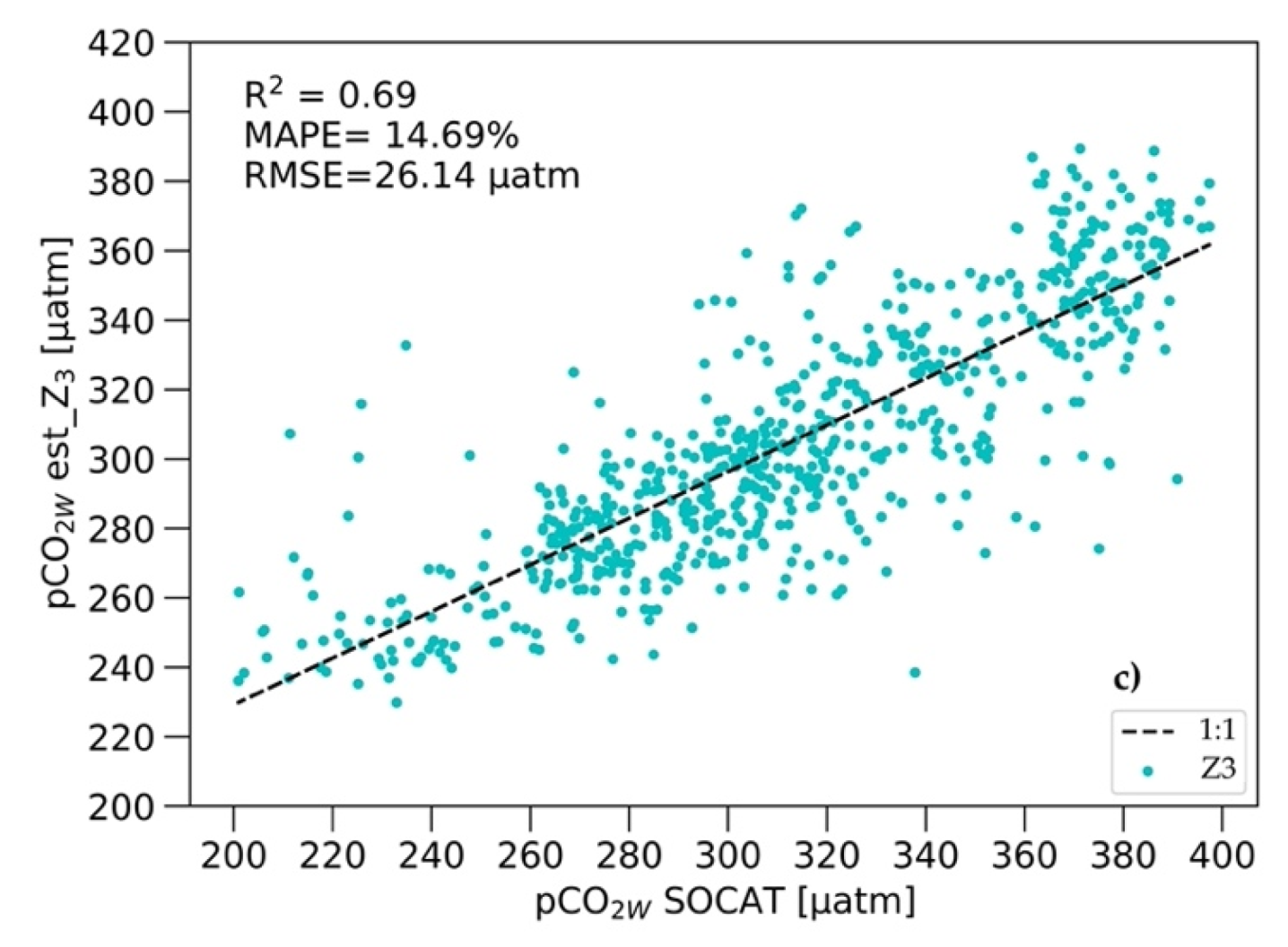
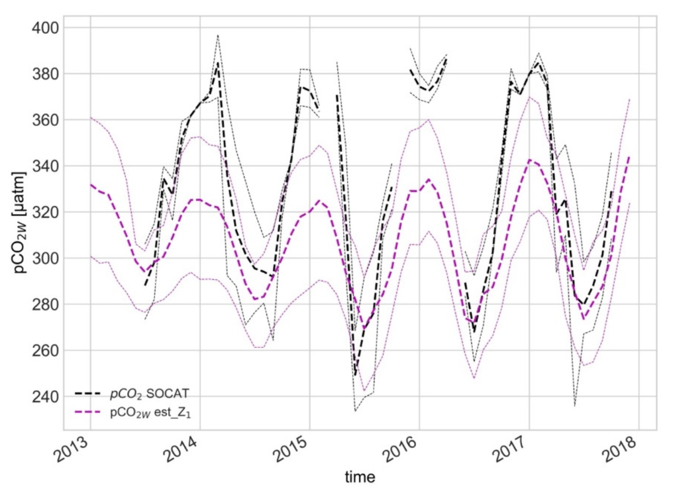
3.1. Estimated pCO_2W Values Based on Three Models

For each observed pCO_2W, the corresponding FFNN pCO_2W was determined based on spatial (1° longitude by 1° latitude grid) and temporal (month intervals between January 2013 and December 2017) coordinates in two models, Z₁ and Z₃, and from March 2013 to November 2017 for Z₂ models. To evaluate the performance of the network-learning processes, we use several statistical parameters: (i) the correlation coefficient (r²); (ii) the standard deviation (σ, µatm) between observed and estimated pCO_2W; (iii) the root-mean-square error (RMSE, µatm) of the observed and estimated pCO_2W; (iv) the mean absolute percentage error (MAPE, %). From 17 results, the best one was chosen based on the RMSE, the r², and MAPE. In our study, these metrics were calculated over the full period as a five-year average.

The scatterplots of estimated pCO_2W versus observed pCO_2W and calculated errors and coefficients highlight the main differences between the three models (Z₁, Z₂, and Z₃; Figure 2). At the EAS scale, the analysis yielded that the r² between estimated and observed pCO_2W increased from 0.69 in model where Chl-a data were excluded to 0.8 in a configuration that includes Chl-a^Y data (Z₁), and the RMSE decreased from 26.14 to 21.19 µatm. With a smaller RMSE and better network fitting, the MAPE increased, and so with an RMSE around 21–22 µatm, the MAPE ranged around 15–16% (Figure 2a,b), while, with a RMSE > 26 µatm, the MAPE was smaller than 15% (Figure 2c). In the Z₁ model, at very low pCO_2W, a lot of outliers occurred, while at higher pCO_2W (>300 µatm), the values were scattered around the identity line for which the correlation coefficient is 1. Despite, the values in Z₁ were more spread than in Z₂ or Z₃, all modeled pCO_2W data from Z₁ were contained in the 25th and 75th percentile of the observed data and RMSE was the lowest. Z₃ models reproduced pCO_2W with the best accuracy in the range 260–340 µatm, while below and above this level, the data were more spread, which was also visible in pCO_2W values distribution reproduced by the Z₂ model, while the Z₂ models only estimated pCO_2W from March to October. Figure 2b shows results from the network after adding Chl-a^S concentrations on a seasonal scale. Comparing results from Z₁ and Z₂ indicated a strong impact of biological activity on pCO_2W distribution in the EAS in winter, as the RMSE of pCO_2W without Chl-a data were 26 µatm; after addition, Chl-a^S decreased to 22 µatm; after including winter values of Chl-a^Y, the RMSE drawdown was about 5 µatm.

The highest pCO_2W values in the continental shelves of the EAS are in the winter, from December to March, when the sea surface temperature is low and solubility of CO₂ in the seawater is high (Figure 3a, black line). In April, when biological activity occurs, sea surface temperature increases, sea surface salinity is reduced by the sea ice melting, and pCO_2W decreases (Figure 3a, black line). In summer (June to August), the EAS waters are strongly vertically stratified, which leads to reductions in the entrainment of CO₂ and nutrients from the depths, so pCO_2W remains low. When vertical stratification declines in October, CO₂ from the sea bottom is carried to the surface [25,49,50,51], and pCO_2W increases (Figure 3a, black line). Despite the better fit and smaller RMSE of estimated pCO_2W from the Z₁ model, the uncertainty of the results from Z₁ and Z₃ were very similar (45 µatm), while the uncertainty of pCO_2W measurements from the Z₂ model was 40 µatm but at a much lower temporal resolution than Z₁ and Z₃. As a validation of the method, we calculated the uncertainty as σ between the modeled values in each model and SOCAT dataset, for our domain. Figure 3 shows comparisons between neural network estimates and observed pCO_2W on a five-year monthly average scale. The best mapping was obtained from model Z₁ (Figure 3a, magenta line); nevertheless, in model Z₃, the network fitted to the observed data was only slightly less good (Figure 3a, blue lines). The dependency and distribution were not reproducing from model Z₂ for November to February because of Chl-a^S concentrations and pCO_2W data gaps. The monthly average values of pCO_2W were underestimated in fall and winter season maxima (October–April), with larger differences than in overestimated summer season minima (June–September), and underestimation was larger when Chl-a data were excluded. From October to April, the biggest differences were also visible between estimated pCO_2W and observed pCO_2W. From March to October, where results from all three models were available, satisfying accuracy between Z₃ (=0.69, Figure 2) and Z₂ (=0.72, Figure 2) models was visible in close pCO_2W values in March, April, and May, while from June to September, monthly distribution from Z₂ was closest to the one from Z₁. Figure 3b represents the σ for monthly average pCO_2W from the three different network models and observed pCO_2W in the EAS. The σ differences between observed pCO_2W and calculated by the FFNN were ± 20 µatm in winter and ± 15 µatm in summer, depending on the model used. Despite the monthly average distribution of observed values being well mapped in all three network models, the σ values varied strongly on an annual scale. The greatest amplitude between modeled and observed pCO_2W was noted in winter (December–March) and was higher than 30 𝜇atm in Z₁, and even higher in Z₃ models. The differences between the estimated pCO_2W and observed pCO_2W were less (Figure 3a) than their σ (Figure 3b). Adding Chl-a data reconstructed for all months (Chl-a^Y) smooths the distribution of pCO_2W (Figure 3a, magenta line) and reduces computational error (Figure 3b magenta line) compared to the distribution where Chl-a from ESA (Chl-a^S) was used (Figure 3a,b, yellow line).

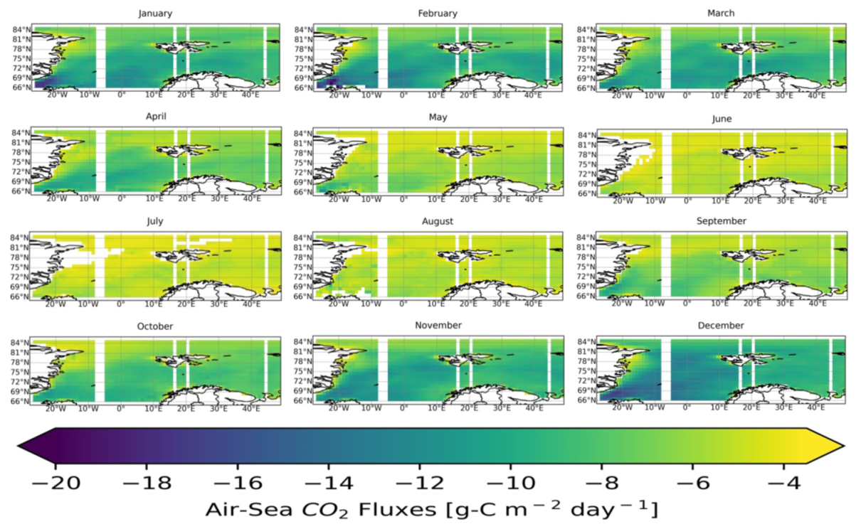
3.2. Spatial pCO_2W and Air-Sea CO₂ Flux Distribution Based on the Z₁ Model

To facilitate a discussion about the temporal variations of pCO_2W in the ESA, Figure 4 shows the time series of average pCO_2W estimated using model Z_1, and observation values with their errors. The estimated pCO_2W values generally agree well with observed values, with most of the data lying within the spatial variability (one the spatial standard deviation: 1σ) calculated for the ESA, especially in the summer season. However, in winter, disagreements in the range of 30–50 µatm between the data occurred, and were about 10–20 µatm in summer. Temporal patterns and variations of modeled data agree well with observed pCO_2W values in the SOCAT dataset. This confirms that the FFNN technique overcomes problems of temporal and spatial data scarcity by putting significant weight on the availability and quality of the training data.

We choose the Z₁ model as a reference model as our analysis has shown it achieves the best network fitting to the observed pCO_2W values (Figure 2). Figure 5 presents pCO_2W values mapped by our network received from rare spatial coverage of the pCO_2W from SOCAT (Supplementary Materials) based on SST, SSS, Chl-a, and MLD. Our network mapped spatial variability very well despite a large lack of target data (Supplementary Materials). In winter (December–March), in a place without sea ice, the CO₂ has high solubility and may be enhanced by the dissolved organic matter carried out during upwelling [48,49], as seen in high pCO_2W values in the Greenland and Norwegian Sea, and the southern part of the Barents Sea (>360 µatm). On an annual basis, these values were the highest in the entire EAS but were nevertheless lower than pCO_2A (five-year mean of 400 µatm) and lower than temporal means (Figure 3a and Figure 4). In winter, the largest amplitudes in the ESA had a latitudinal distribution increasing from west to east, about 100 µatm along parallels (Figure 5). A tongue of very high pCO_2W initially reaching the coast of Novaya Zemlya, still visible in May near Novaya Zemlya, completely lapsed in June. The exception was the east coast of Greenland, where pCO_2W was still at the 320–340 µatm level. In spring (April–June), when carbon dissolved in seawater is converted into the organic matter photosynthesis, simplistically, pCO_2W decreased in the Greenland and Norwegian Sea (about around 30–40 µatm below the winter level) and leveled off throughout the EAS basin (<320 µatm). Summer stratification of the Arctic Ocean waters and the intensive carbon consumption by algae to conduct photosynthesis resulting in low pCO_2W (<280 µatm) were very well reproduced by our network model. The difference in values along the parallels was not as great as in winter and occurred only between the water along the east coast of Greenland and the rest of the basin. In fall (October–December), pCO_2W values increased from the summer level, as thermocline dissolved and carbon from the deep sea reached the sea surface through upwelling.

The continental shelf of the European Arctic Sector is characterized by low CO₂ concentration in seawater during spring and summer, largely due to strong biological uptake driven by extensive plankton blooms in spring [52,53]. Both carbon exchange fluxes and the accumulation of organic carbon in marine systems are controlled by a variety of mechanisms. For those mechanisms, we included primary production of the surface waters, runoff of terrigenous organic matter through the rivers from the continents, biogeochemical processes in the water column and at the seafloor, and the sedimentation rate. We calculated the five-year monthly mean of Air-Sea CO₂ fluxes based on the pCO_2W difference calculated from our FFNN model and gas transfer coefficient calculated from the wind speed. The five-year monthly mean CO₂ flux distribution shows that all continental shelf areas of the Arctic Ocean were net CO₂ sinks (Figure 6). Strong monthly CO₂ influx to the Arctic Ocean through the Greenland and Barents Seas (>12 gC m⁻² day⁻¹) occurred in the fall and winter, when the pCO_2W level at the sea surface was high (>360 µatm), and featured the strongest wind speed (>12 ms⁻¹; [9]). In contrast, there was a weak influx in the summer (~4 gC m⁻² day⁻¹). Our monthly CO₂ flux is consistent with those reported by most previous studies [17,19,20,25]. The five-year annual mean was around 10–20 gC m⁻² day⁻¹. The EAS, as a whole, is a sink of CO₂, but in some regions, close to North Atlantic Drift and East Greenland Current, weak sinks exist (Figure 6). Our estimates are similar to those obtained by [9] for the same region. Waters along the east Greenland coast, despite a high pCO_2W level (Figure 5), were weaker sinks than the Barents Sea.

4. Discussion

We tested the feed-forward neural network with three different models to diagnose monthly and seasonal ocean surface pCO₂ fields from 2013 to 2017 in the continental shelf areas of the European Arctic Sector (the Greenland, Norwegian, and Barents seas). We chose this region because it is one of the most complicated regions, smaller than the Arctic Ocean or the North Atlantic, with a relatively large amount of data availability. We assessed how accurately the three neural network models could reproduce the observed pCO_2W calculated from Surface Ocean Carbon Atlas (SOCAT) by comparing their r², RMSE, MAPE, and σ. Scatterplots highlight the main differences between the three models (Figure 2), and show that the model which contains Chl-a concentration from re-analysis (Chl-a^Y), sea surface temperature (SST), salinity (SSS), and the upper ocean mixed–layer depth (MLD) as a target to predict the spatiotemporal distribution of pCO_2W in the sea surface gives the best results and best-fitting network to the observational data (Figure 2a), despite the higher spread of the values than in other models. As a validation of the method, for our domain we calculated the uncertainty as σ between the modeled values in each model and SOCAT dataset. Surprisingly, the uncertainties from the Z₁ model were similar to those from the Z₃ model, which did not contain Chl-a concentration data (45 µatm). The RMSE calculated for the reconstructed pCO_2W values in all three models gave lower values than the measurement uncertainties calculated for pCO_2W: respectively, RMSE: Z₁ = 21.19 µatm, Z₂ = 22.46 µatm, Z₃ = 26.14 µatm (Figure 2); uncertainty (σ): Z₁ and Z₃ = 45 µatm and Z₂ = 40 µatm. The uncertainty of the pCO_2W measurements calculated in model Z₂ appears to be smaller than in models Z₁ or Z₃, but the temporal resolution in model Z₂ was much lower than in the others because the network did not interpolate the pCO_2W values for December–March in model Z₂. pCO_2W values from all models are within the 25th and 75th percentile. The high biological CO₂ uptake in shallow stratified layers during the spring bloom, resulting in rapid CO₂ drawdown in the surface waters of the EAS, was visible as a rapid pCO_2W drawdown in Figure 3. The authors of [37,54] identified that the SST is always the main parameter influencing the pCO_2W distribution, whereas Chl-a is the second parameter in the winter and MLD in the fall. Additionally, [54] identified a linear relationship between the MLD from the beginning of the bloom until the MLD deepening in fall. The correlation coefficient for the five–year pCO_2W mean in model Z₁ was close to the correlation coefficient in the summer and fall in the North Atlantic in [37] calculated from their Equation (3), where they estimated pCO_2W using SST, Chl-a, and MLD as predictors in the multiple regression. The correlation coefficient from model Z₃, in our study, was similar to those for winter from Equation (4) in [37], where only SST, lat, and lon were included, and additionally, the result from model Z₂ was similar to results from Equation (2) in the spring and summer in [37], where only SST was used as a predictor to estimation pCO_2W distribution. Our calculation of monthly drivers of the estimated pCO_2W change within continental shelf areas of the EAS confirms a major impact not only on the biological effects to the pCO_2W distribution (Figure 5) and Air-Sea CO₂ flux in the EAS (Figure 6), but also mixing of the upper ocean layer. It also indicates that strong seasonal correlations between the predictor and pCO_2W, seen earlier in the North Atlantic, are strongly visible as a year correlation in the EAS. In addition, it indicated the possibility of using Chl-a^Y data, taking into account overestimated modeled results with higher bias, which did not affect the quality of network fitting. The RMSE from our network was comparable to those obtained from [23] for the assessment of a pCO_2W distribution based on the FFNN method (for the Arctic, respectively, RMSE of 22.05 µatm; Table 1 in [23]). This also confirms that the calculated pCO_2W quantitatively and qualitatively reproduced the original pCO_2W data when the biological process and mixing of the upper ocean layer was included. In a recent study, [21] prepared monthly maps of Air-Sea CO₂ fluxes from 1997 to 2014 for the Arctic Ocean and its adjacent seas by applying the Self-Organizing Maps (SOM) technique to map pCO_2W with SST, SSS, SIC, Chl-a, and atmospheric CO₂ mixing ratio values. They reported that adding a biological effect for mapping pCO_2W reduces the uncertainty and calculated the basin-wide RMSE at 30 µatm and r² equal to 0.82. Results from our FFNN were smaller than those obtained by [21], which was surprising, as we expected larger errors due to a much smaller area and, therefore, a smaller amount of pCO_2w data. This confirmed the ability of the network to model pCO_2W with high accuracy (r > 0.8) based on a very small database, but it also appeared to indicate that on a monthly average scale, adding Chl-a concentrations to the network of estimated pCO_2W in the EAS improves model fit. Monthly pCO_2W values for 2013–2017 were lower than those indicated by [15]. The spatial distribution of monthly mean pCO_2W (Figure 5) was in good agreement with [20,21] results. The estimated pCO_2W and Air-Sea CO₂ flux were lower in the Greenland and Barents seas than in the Norwegian Sea, except that the longitudinal differences between pCO_2W were higher than longitudinal differences of Air-Sea CO₂ flux. To enhance the importance of the seasonality, we considered using cosine and sine functions for a time, as [13,18] had. We tested the network with cos/sin time as a predictor and compared it with the network, where the time was not periodically functioned. The results with cos/sin were considerably higher, and estimated target values were outside the scope of recognition.

The five-year annual mean CO₂ flux distribution shows that all areas of the continental shelf of the EAS were a net sink. During the year, the calculated pCO_2W shows a seasonal variation of about 100 µatm, with two maxima in March and November, and a minimum from June to August (Figure 3a). The standard deviation between observed pCO_2W values and estimated in model Z₁ was higher in the winter and fall, where in addition to SST, the distribution of pCO_2W is influenced by biological activity and the upper ocean mixing, compared to the summer, wherein the EAS vertical stratification is visible, and CO₂ was drawn down by the algae (Figure 3a). Our modeled data uncertainty, calculated as their σ, of the individual parameters was 38% for k calculations using [42]’s parameterization, for a wind speed of 16%, and 35% for pCO_2W and 29% for pCO_2A, which we compared to those calculated by [20]—36, 11, 32%—adequately. However, it is important to note that their uncertainties were for the entire Arctic Ocean, while we focus on a smaller domain, and the comparison is only between the values we obtained and those calculated by [20], not on the basis of in-depth comparative analysis of the data. The σ provided an estimate of the uncertainty of the method in reproducing the in situ measurements. The compared values mean that our uncertainties were smaller, which may confirm that using FFNN for model pCO_2W in the EAS as a component to estimate Air-Sea CO₂ flux in this region is as good as using SOM, but more in-depth analyses are necessary based on the uncertainties of both methods.

5. Conclusions

We aimed to verify how the FFNN worked with estimated pCO_2W over the EAS using sea-surface temperature (SST), sea-surface salinity (SSS), upper ocean mixing-layer depth (MLD), chlorophyll-a concentrations (Chl-a), latitude, longitude, and time as predictors while applying different approaches to the Chl-a data (Z₁), (Z₂) and excluding Chl-a data from the network (Z₃). To enhance the importance of the seasonality, we considered using cosine and sine functions for a month, as [13,18] had. We tested the network with cos/sin for a time as a predictor and compared it with network, where the time was not periodically functioned. The results were considerably higher, and estimated target values were outside the scope of recognition in network with cos/sin. This means that it is unnecessary to use sine and cosine functions for a time for estimating pCO_2W in a small area. The network based on the available prediction data for the EAS predicts all temporal fluctuations occurring in high northern latitudes with accuracy at a satisfying level (r > 0.6), acceptable uncertainty (35% for pCO_2W from Z₁ model), and 15% bias between modeled and observed pCO_2W data in the scale of the EAS. Adding spatial and temporal resolution to the study of pCO_2W by using an FFNN, on the scale of the EAS, helped to improve the results and accuracy of the network. On the pCO_2W distribution and Air-Sea CO₂ flux in the EAS, a major impact has not only SST and Chl-a concentrations but also mixing of the upper ocean layer. The EAS climatology was predicted with satisfactory accuracy, with an RMSE of 21.19 µatm in the model in which Chl-a data from re-analysis were used, to 22.46 µatm for the model in which Chl-a data were from ESA. Higher RMSE values of about 26.14 µatm were noted in the model in which Chl-a data were excluded. The five-year monthly mean CO₂ flux distribution shows that all continental shelf areas of the Arctic Ocean were net CO₂ sinks, and strong monthly CO₂ influx through the Greenland and Barents Seas (>12 gC m⁻² day⁻¹) occurred in the fall and winter, when the pCO_2W level at the sea surface was high (>360 µatm).

References

1. Global Monitoring Laboratory, Mauna Loa. Available online: https://gml.noaa.gov/dv/iadv/graph.php?code=MLO&program=ccgg&type=ts (accessed on 14 February 2021).
2. Sabine, C.L.; Feely, R.A.; Gruber, N.; Key, R.M.; Lee, K.; Bullister, J.L.; Wanninkhof, R.; Wong, C.S.; Wallace, D.W.R.; Tilbrook, B.; et al. The Oceanic sink for anthropogenic CO2. Science 2004, 305, 367–371. [Google Scholar] [CrossRef] [Green Version]
3. Le Quéré, C.L.; Takahashi, T.; Buitenhuls, E.; Rödenbeck, C.; Sutherland, S.C. Impact of climate change and variability on the global oceanic sink of CO2. Global Biogeochem. Cycles 2010, 24. [Google Scholar] [CrossRef] [Green Version]
4. Gregor, L.; Kok, S.; Monteiro, P.M.S. Empirical methods for the estimation of Southern Ocean CO2: Support vector and random forest regression. Biogeosciences 2017, 14, 5551–5569. [Google Scholar] [CrossRef] [Green Version]
5. Watson, A.J.; Schuster, U.; Shutler, J.D.; Holding, T.; Ashton, I.G.C.; Landschützer, P.; Woolf, D.K.; Goddijn-Murphy, L. Revised estimates of ocean-atmosphere CO2 flux are consistent with ocean carbon inventory. Nat. Commun. 2020, 11, 4422. [Google Scholar] [CrossRef]
6. Friedlingstein, P.; Jones, M.W.; O’Sullivan, M.; Andrew, R.M.; Hauck, J.; Peters, G.P.; Peters, W.; Pongratz, J.; Sitch, S.; Le Quéré, C.; et al. Global carbon budget 2019. Earth Syst. Sci. Data 2019, 11, 1783–1838. [Google Scholar] [CrossRef] [Green Version]
7. Woolf, D.K.; Shutler, J.D.; Goddijn-Murphy, L.; Watson, A.J.; Chapron, B.; Nightingale, P.D.; Donlon, C.J.; Piskozub, J.; Yelland, M.J.; Ashton, I.; et al. Key uncertainties in the recent air-sea flux of CO2. Glob. Biogeochem. Cycles 2019, 33, 1548–1563. [Google Scholar] [CrossRef] [Green Version]
8. Doney, S.C.; Fabry, V.J.; Feely, R.A.; Kleypas, J.A. Ocean Acidification: The other CO2 problem. Ann. Rev. Mar. Sci. 2009, 1, 169–192. [Google Scholar] [CrossRef] [Green Version]
9. Wrobel, I.; Piskozub, J. Effect of gas-transfer-velocity parameterizations choice on air-sea CO2 fluxes in the North Atlantic and the European Arctic. Ocean Sci. 2016, 12, 1091–1103. [Google Scholar] [CrossRef] [Green Version]
10. Cooper, D.J.; Watson, A.J.; Ling, R.D. Variation of pCO2 along a North Atlantic shipping route (U.K. to the Caribbean): A year of automated observations. Mar. Chem. 1998, 60, 147–164. [Google Scholar] [CrossRef]
11. Bates, N.R.; Mathis, J.T. The Arctic Ocean marine carbon cycle: Evaluation of air-sea CO2 exchanges, ocean acidification impacts and potential feedbacks. Biogeosciences 2009, 6, 2433–2459. [Google Scholar] [CrossRef] [Green Version]
12. Bates, N.R.; Michaels, A.F.; Knap, A.H. Seasonal and interannual variability of oceanic carbon dioxide species at the U.S. JGOFS Bermuda Atlantic Time-Series Study (BATS) site. Deep-Sea Res. II 1996, 43, 347–383. [Google Scholar] [CrossRef]
13. Lefèvre, N.; Watson, A.J.; Watson, A.R. A comparison of multiple regression and neural network techniques for mapping in situ pCO2 data. Tellus B 2005, 57, 375–384. [Google Scholar] [CrossRef]
14. Cai, W.-J.; Dai, M.; Wang, Y. Air-sea exchange of carbon dioxide in ocean margins: A province-based synthesis. Geophys. Res. Lett. 2006, 33, L12603. [Google Scholar] [CrossRef] [Green Version]
15. Telszewski, M.; Chazottes, A.; Schuster, U.; Watson, A.J.; Moulin, C.; Bakker, D.C.E.; González-Dávila, M.; Johannessen, T.; Körtzinger, A.; Lüger, H.; et al. Estimating the monthly pCO2 distribution in the North Atlantic using a self-organizing neural network. Biogeosciences 2009, 6, 1405–1421. [Google Scholar] [CrossRef] [Green Version]
16. Landschützer, P.; Gruber, N.; Bakker, D.C.E.; Schuster, U.; Nakaoka, S.; Payne, M.R.; Sasse, T.; Zeng, J. A neural network-based estimate of the seasonal to inter-annual variability of the Atlantic Ocean carbon sink. Biogeosciences 2013, 10, 7793–7815. [Google Scholar] [CrossRef] [Green Version]
17. Takahashi, T.; Sutherland, S.C.; Wanninkhof, R.; Sweeney, C.; Feely, R.A.; Chipman, D.W.; Hales, B.; Friederich, G.; Chavez, F.; Sabine, C.; et al. Climatological mean and decadal change in surface ocean pCO2 and net sea-air CO2 flux over the global oceans. Deep-Sea Res. Pt. II 2009, 56, 554–577. [Google Scholar] [CrossRef]
18. Friedrich, T.; Oschlies, A. Neural network-based estimates of North Atlantic surface pCO2 from satellite data: A methodological study. J. Geophys. Res. 2009, 114, C03020. [Google Scholar] [CrossRef] [Green Version]
19. Nakaoko, S.; Telszewski, M.; Nojiri, Y.; Yasunaka, S.; Miyazaki, C.; Mukai, H.; Usui, N. Estimating temporal and spatial variation of ocean surface pCO2 in the North Pacific using a self-organizing map neural network technique. Biogeosciences 2012, 10, 6093–6106. [Google Scholar] [CrossRef] [Green Version]
20. Yasunaka, S.; Murata, A.; Watanabe, E.; Chierici, M.; Fransson, A.; van Heuven, A.; Hoppema, M.; Ishii, M.; Johannessen, T.; Kosugi, N.; et al. Mapping of the air-sea CO2 flux in the Arctic Ocean and its adjacent seas: Basin-wide distribution and seasonal to interannual variability. Polar Sci. 2016, 10, 323–334. [Google Scholar] [CrossRef]
21. Yasunaka, S.; Siswanto, E.; Olsen, A.; Hoppema, M.; Watanabe, E.; Fransson, A.; Chierici, M.; Murata, A.; Lauvset, S.K.; Wanninkhof, R.; et al. Arctic Ocean CO2 uptake: An improved multiyear estimate of the air-sea CO2 flux incorporating chlorophyll-a concentrations. Biogeosciences 2018, 15, 1643–1661. [Google Scholar] [CrossRef] [Green Version]
22. Laruelle, G.G.; Landschützer, P.; Gruber, N.; Tison, J.-L.; Delille, B.; Regnier, P. Global high-resolution monthly pCO2 climatology for the coastal ocean derived from neural network interpolation. Biogeosciences 2017, 14, 4545–4561. [Google Scholar] [CrossRef] [Green Version]
23. Denvil-Sommer, A.; Gehlen, M.; Vrac, M.; Mejia, C. LSCE-FFNN-v1: A two-step neural network model for the reconstruction of surface ocean pCO2 over the global ocean. Geosci. Model Dev. 2019, 12, 2091–2105. [Google Scholar] [CrossRef] [Green Version]
24. Longhurst, A.; Sathyendranath, S.; Platt, T.; Cavarhill, C. An estimate of global primary production in the ocean from satellite radiometer data. J. Plankton Res. 1995, 17, 1245–1271. [Google Scholar] [CrossRef] [Green Version]
25. Wrobel, I. Monthly dynamics of carbon dioxide exchange across the sea surface of the Arctic Ocean in response to changes in gas transfer velocity and partial pressure of CO2 in 2010. Oceanologia 2017, 59, 445–459. [Google Scholar] [CrossRef]
26. Chierici, M.; Olse, A.; Johannessen, T.; Trinañes, J.; Wanninkhof, R. Algorithms to estimate the carbon dioxide uptake in the northern North Atlantic using shipboard observations, satellite and ocean analysis data. Deep-Sea Res. Pt. II 2009, 56, 630–639. [Google Scholar] [CrossRef]
27. Bakker, D.C.E.; Pfeil, B.; Landa, C.S.; Metzl, N.; O’Brien, K.M.; Olsen, A.; Smith, K.; Cosca, C.; Harasawa, S.; Jones, S.D.; et al. Multi-decade record of high-quality fCO2 data in version 3 of the Surface Ocean CO2 Atlas (SOCAT). Earth Syst. Sci. Data 2016, 8, 383–413. [Google Scholar] [CrossRef] [Green Version]
28. Körtzinger, A. Determination of carbon dioxide partial pressure (pCO2). In Methods of Seawater Analysis, 3rd ed.; Grasshoff, K., Kremling, K., Ehrhardt, M., Eds.; Wiley: Weinheim, Germany, 1999. [Google Scholar] [CrossRef]
29. Copernicus Marine Environment Services. Available online: https://resources.marine.copernicus.eu/?option=com_csw&view=details&product_id=GLOBAL_R153 EANALYSIS_PHY_001_026 (accessed on 10 February 2020).
30. Forget, G.; Campin, J.M.; Heimbach, P.; Hill, C.N.; Ponte, R.M.; Wunsch, C. ECCO version 4: AN integrated framework for non-linear inverse modelling and global ocean state estimation. Geoscientific Model Dev. 2015, 8, 3071–3104. Available online: https://ecco-group.org/products.htm (accessed on 10 February 2020). [CrossRef] [Green Version]
31. Copernicus Marine Environment Services. Available online: https://resources.marine.copernicus.eu/?option=com_csw&view=details&product_id=GLOBAL_R172 EANALYSIS_BIO_001_029 (accessed on 10 February 2020).
32. Copernicus Marine Environment Services, NEMO Modeling Platform. Available online: https://resources.marine.copernicus.eu/documents/QUID/CMEMS-GLO-QUID-001-029.pdf (accessed on 10 February 2020).
33. European Space Agency/GlobColour Program. Available online: https://hermes.acri.fr (accessed on 10 February 2020).
34. Maritorena, S.; Siegel, D.A. Consistent merging of satellite ocean colour data sets using a bio-optical model. Remote Sens. Environ. 2005, 94, 429–440. [Google Scholar] [CrossRef]
35. Kohonen, T. Self-organized formation of topologically correct feature maps. Biol. Cybern. 1982, 43, 59–69. [Google Scholar] [CrossRef]
36. Keras. Available online: https://keras.io (accessed on 15 November 2021).
37. Jamet, C.; Moulin, C.; Lefèvre, N. Estimation of oceanic pCO2 in the North Atlantic from VOS lines in-situ measurements: Parameters need to generate seasonally mean maps. Ann. Geophys. 2007, 25, 2247–2257. [Google Scholar] [CrossRef] [Green Version]
38. Dlugokencky, E.J.; Mund, J.W.; Crotwell, A.M.; Crotwell, M.J.; Thoning, K.W. Atmospheric Carbon Dioxide Air Mole Fractions from the NOAA GML Carbon Cycle Cooperative Global Air Sampling Network, 2021, pp. 1968–2020. Available online: https://gml.noaa.gov/aftp/data/trace_gases/co2/flask/surface/README_surface_flask_co2.html (accessed on 30 July 2021).
39. Goddijn-Murphy, L.; Woolf, D.K.; Callaghan, A.H.; Nightingale, P.D.; Shutler, J.D. A reconciliation of empirical and mechanistic models of the air-sea gas transfer velocity. J. Geophys. Res. 2016, 121, 818–835. [Google Scholar] [CrossRef] [Green Version]
40. Weiss, R.F. Carbon dioxide in water and seawater: The solubility of a non-ideal gas. Mar. Chem. 1974, 2, 203–215. [Google Scholar] [CrossRef]
41. Weiss, R.F.; Price, B.A. Nitrous oxide solubility in water and seawater. Mar. Chem. 1980, 8, 347–359. [Google Scholar] [CrossRef]
42. Nightingale, P.D.; Malin, G.; Law, C.S.; Watson, A.J.; Liss, P.S.; Liddicoat, M.I.; Boutin, J.; Upstill-Goddard, R.C. In situ evaluation of air-sea gas exchange parameterizations using novel conservative and volatile tracers. Glob. Biogeochem. Cycles 2000, 14, 373–387. [Google Scholar] [CrossRef]
43. Wanninkhof, R. Relationship between wind speed and gas exchange over the ocean. J. Geophys. Res. 1992, 97C5, 7373–7382. [Google Scholar] [CrossRef]
44. Ho, D.T.; Law, C.S.; Smith, M.J.; Schlosser, P.; Harvey, M.; Hill, P. Measurements of air-sea gas exchange at high wind speeds in the Southern Ocean: Implications for global parameterizations. Geophys. Res. Lett. 2006, 33, 16611. [Google Scholar] [CrossRef] [Green Version]
45. Wanninkhof, R.; McGillis, W.R. Relationship between wind speed and gas exchange over the ocean revisited. Limnol. Oceanogr. Meth. 2014, 12, 351–362. [Google Scholar] [CrossRef]
46. Wanninkhof, R.; McGillis, W.R. A cubic relationship between air-sea CO2 exchange and wind speed. Geophys. Res. Lett. 1999, 26, 1889–1892. [Google Scholar] [CrossRef]
47. McGillis, W.R.; Edson, J.B.; Hare, J.R.; Fairall, C.W. Direct covariance air-sea CO2 fluxes. J. Geophys. Res. 2001, 106, 16729–16745. [Google Scholar] [CrossRef]
48. Couldrey, M.P.; Oliver, K.I.C.; Yool, A.; Halloran, P.R.; Achterberg, E.R. On which timescale do gas transfer velocities control North Atlantic CO2 flux variability? Global Biogeochem. Cyc. 2016, 30, 787–802. [Google Scholar] [CrossRef] [Green Version]
49. Arrigo, K.R.; van Dijken, G.; Pabi, S. Impact of shrinking Arctic ice cover on marine primary production. Geophys. Res. Lett. 2008, 35, LI9603. [Google Scholar] [CrossRef]
50. Arrigo, K.R.; Pabi, S.; van Dijken, G.L.; Maslowski, W. Air-sea flux of CO2 in the Arctic Ocean, 1998–2003. J. Geophys. Res. 2010, 115, G04024. [Google Scholar] [CrossRef]
51. Arrigo, K.R.; Perovich, D.K.; Pickart, R.S.; Brown, Z.W.; van Dijken, G.L.; Lowry, K.E.; Mills, M.M.; Palmer, M.A.; Balch, W.M.; Bahr, F.; et al. Massive phytoplankton blooms under Arctic sea ice. Science 2012, 336, 1408. [Google Scholar] [CrossRef] [PubMed] [Green Version]
52. Chen, M.; Kim, J.-H.; Nam, S.-I.; Niessen, F.; Hong, W.-L.; Kand, M.-H.; Hur, J. Production of fluorescent dissolved organic matter in Arctic Ocean sediments. Sci. Rep. 2016, 6, 39213. [Google Scholar] [CrossRef] [PubMed] [Green Version]
53. Lønborg, C.; Carreira, C.; Jickells, T.; Álvarez-Salgado, X.-A. Impacts of global change on ocean dissolved organic carbon (DOC) Cycling. Front. Mar. Sci. 2020, 7, 466. [Google Scholar] [CrossRef]
54. Olsen, A.; Brown, K.R.; Chierici, M.; Johannessen, T.; Neill, C. The sea surface CO2 fugacity and its relationship with environmental parameters in the subpolar North Atlantic 2005. Biogeosci. Disc. 2007, 4, 1737–1777. [Google Scholar]
Figure 1. Map of the European Arctic and its adjacent seas.
Remotesensing 14 00312 g001
Figure 2. Scatter plot of estimated pCO2W vs. observed pCO2W obtained based on three models: (a) Z1; (b) Z2; (c) Z3 for 2013–2017 (𝜇atm).
Remotesensing 14 00312 g002aRemotesensing 14 00312 g002b
Figure 3. (a) Climatological monthly average of observed pCO2W (black) and estimated pCO2W over grid boxes for which observed pCO2W values were available; (b) monthly average of the σ between observed (black) and estimated pCO2W.
Remotesensing 14 00312 g003
Figure 4. Monthly mean of pCO2W from SOCAT (black) and estimated using the Z1 model (magenta) in the European Arctic Sector with errors.
Remotesensing 14 00312 g004
Figure 5. Five-year monthly average distribution of pCO2W in the European Arctic Sector.
Remotesensing 14 00312 g005
Figure 6. Five-year annual monthly mean of Air-Sea CO2 fluxes based on pCO2W (µatm) from Z1 models in the European Arctic Sector.
Remotesensing 14 00312 g006