
On-Orbit Radiometric Calibration of Hyperspectral Sensors on Board Micro-Nano Satellite Constellation Based on RadCalNet Data

 ,
,  ,
,  ,
,
Abstract
:
1. Introduction
2. Materials and Methods
2.1. Satellite Constellation and RadCalNet Sites
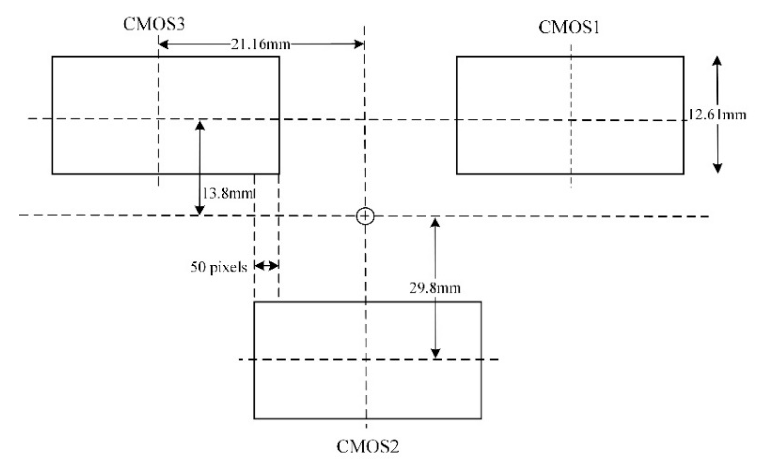
2.1.1. The Zhuhai-1 Constellation and Hyperspectral Sensors
2.1.2. RadCalNet Sites
2.2. Methods
2.2.1. The Proposed Calibration Method for OHS
- The regions of interest (ROIs) are extracted from OHS images over RadCalNet sites, and the surface reflectance and atmosphere parameters, such as AOD, WCV, and ozone content, are also extracted from the RadCalNet product.
- Then, the Second Simulation of the Satellite Signal in the Solar Spectrum (6S) radiative transfer (RT) model [18] is used to simulate the TOA radiance, which will be used with the DN value to calculate the comprehensive gains.
- An adaptive weighted least squares method is used to solve the comprehensive gains, and then, they will be evaluated. The absolute radiometric correction is carried out using the fitting comprehensive gains to obtain the TOA radiance.
- The atmosphere correction is then conducted to obtain the retrieved surface reflectance, which is compared to the ground measured reflectance. The closer they are, the more accurate the comprehensive gains are.
2.2.2. RadCalNet Data Process
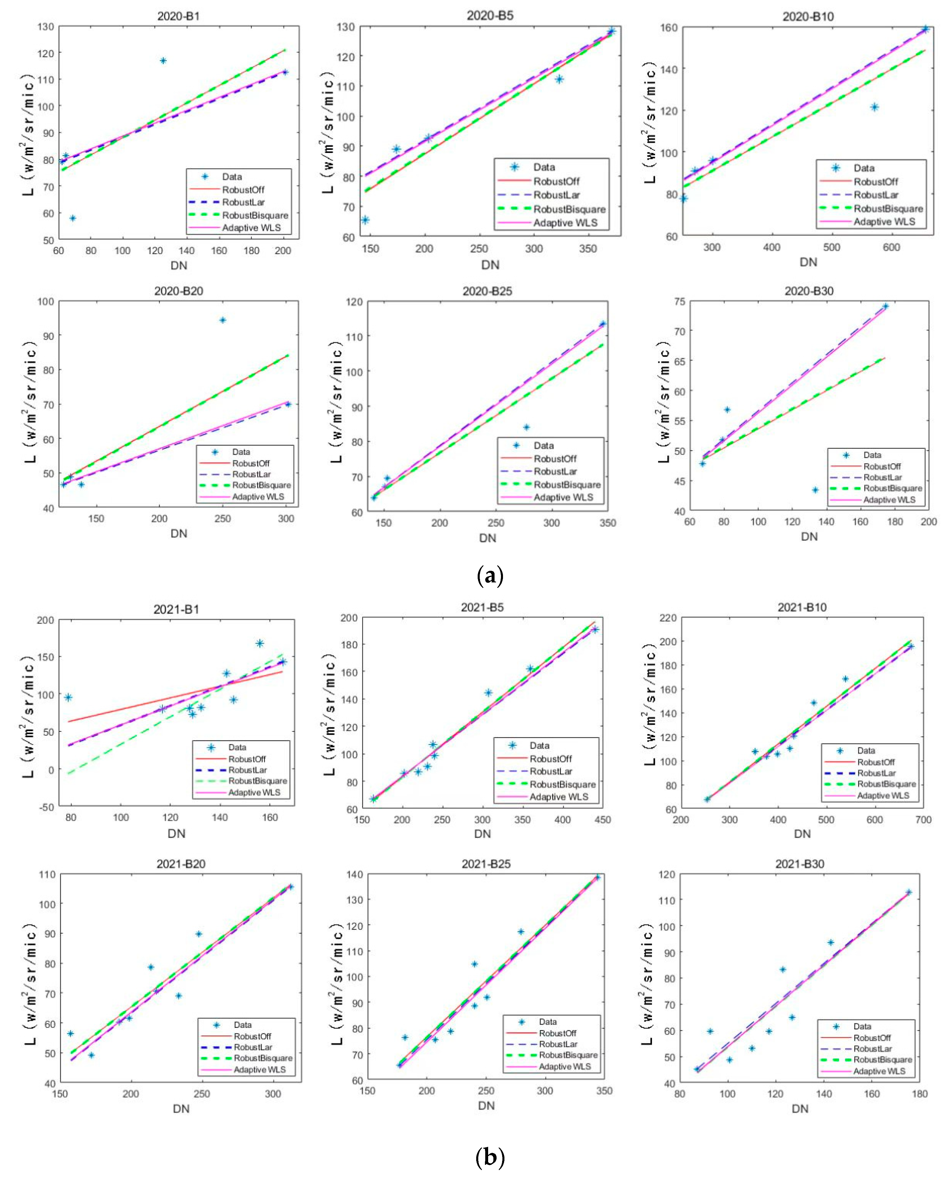
2.2.3. Comprehensive Gain Calculation
2.2.4. Evaluation Method of Calibration Results
3. Results
3.1. Stability Analysis of Multi-Temporal Calibration Results
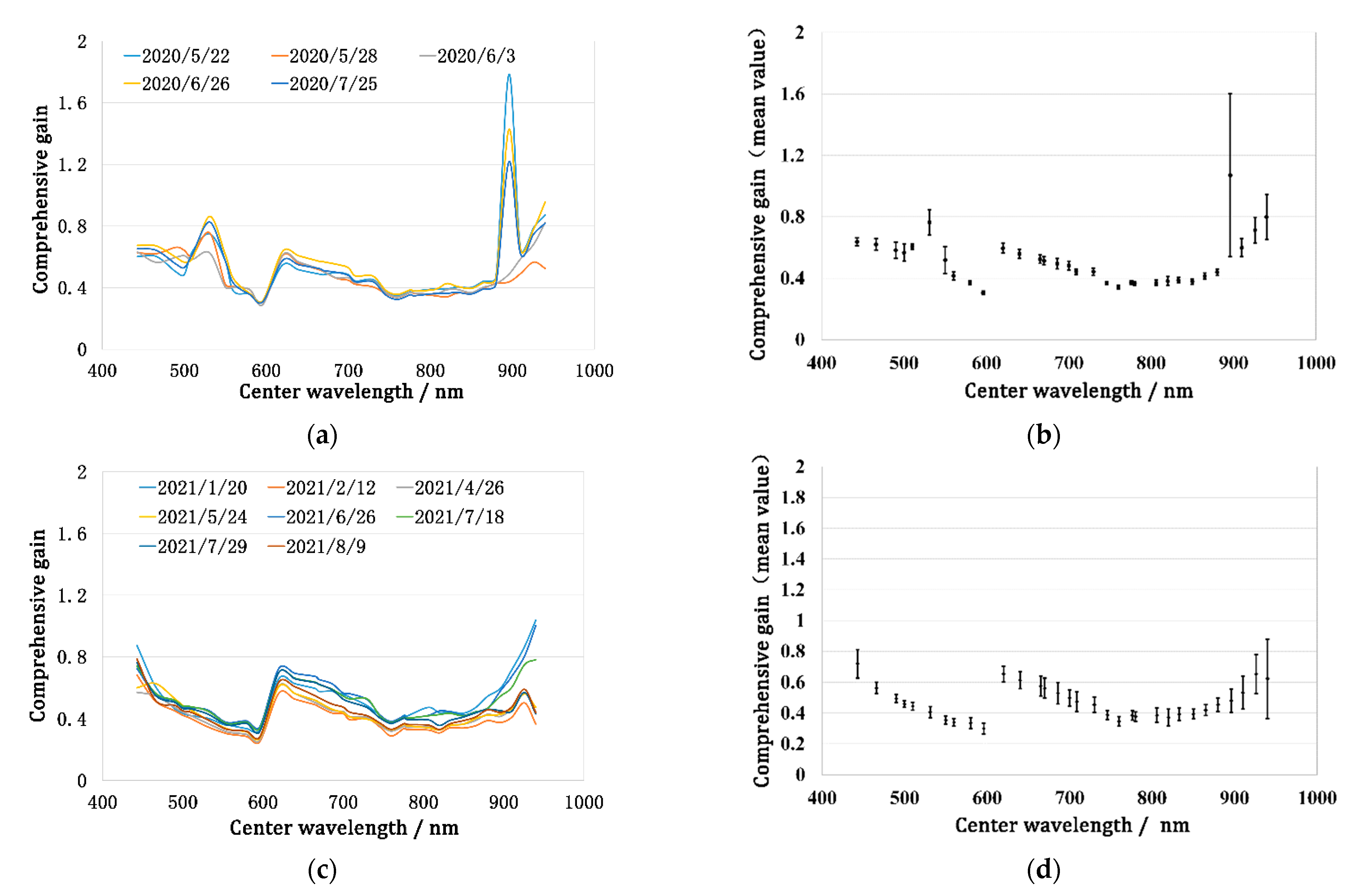
3.1.1. OHS-F CMOS1 Calibration Results and Analysis
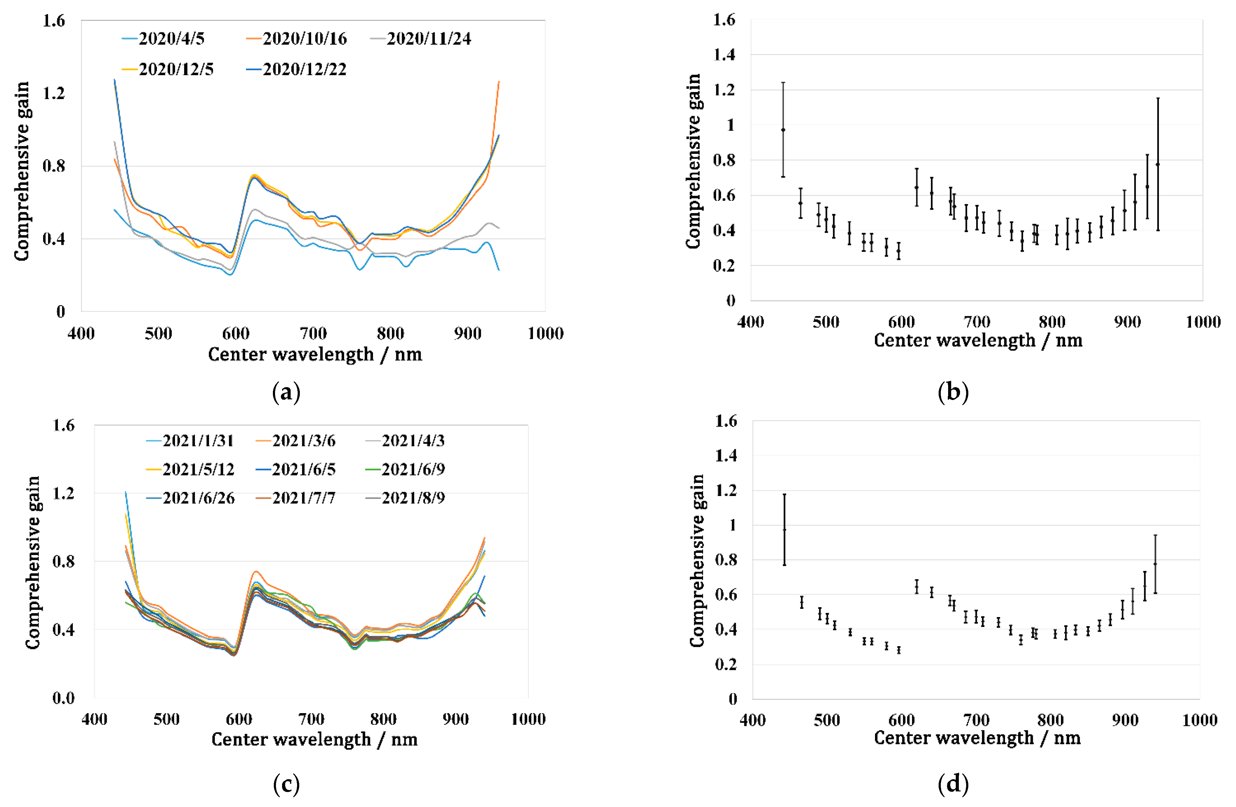
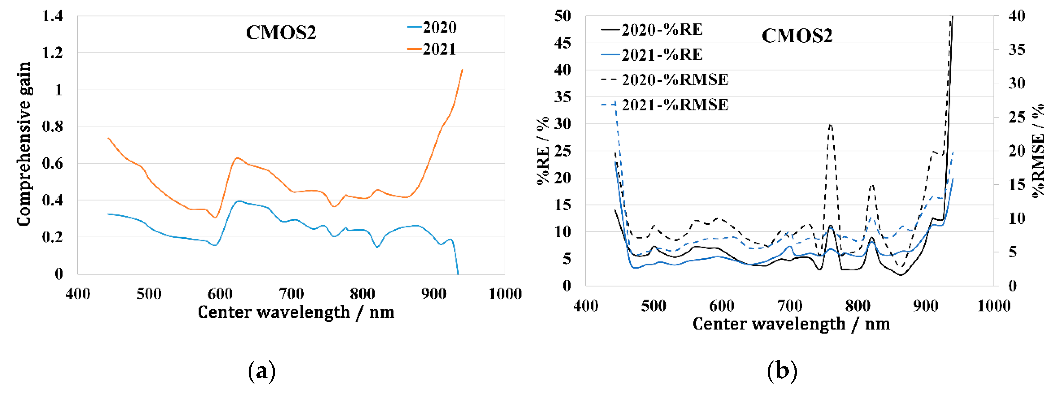
3.1.2. OHS-F CMOS2 Calibration Results and Analysis
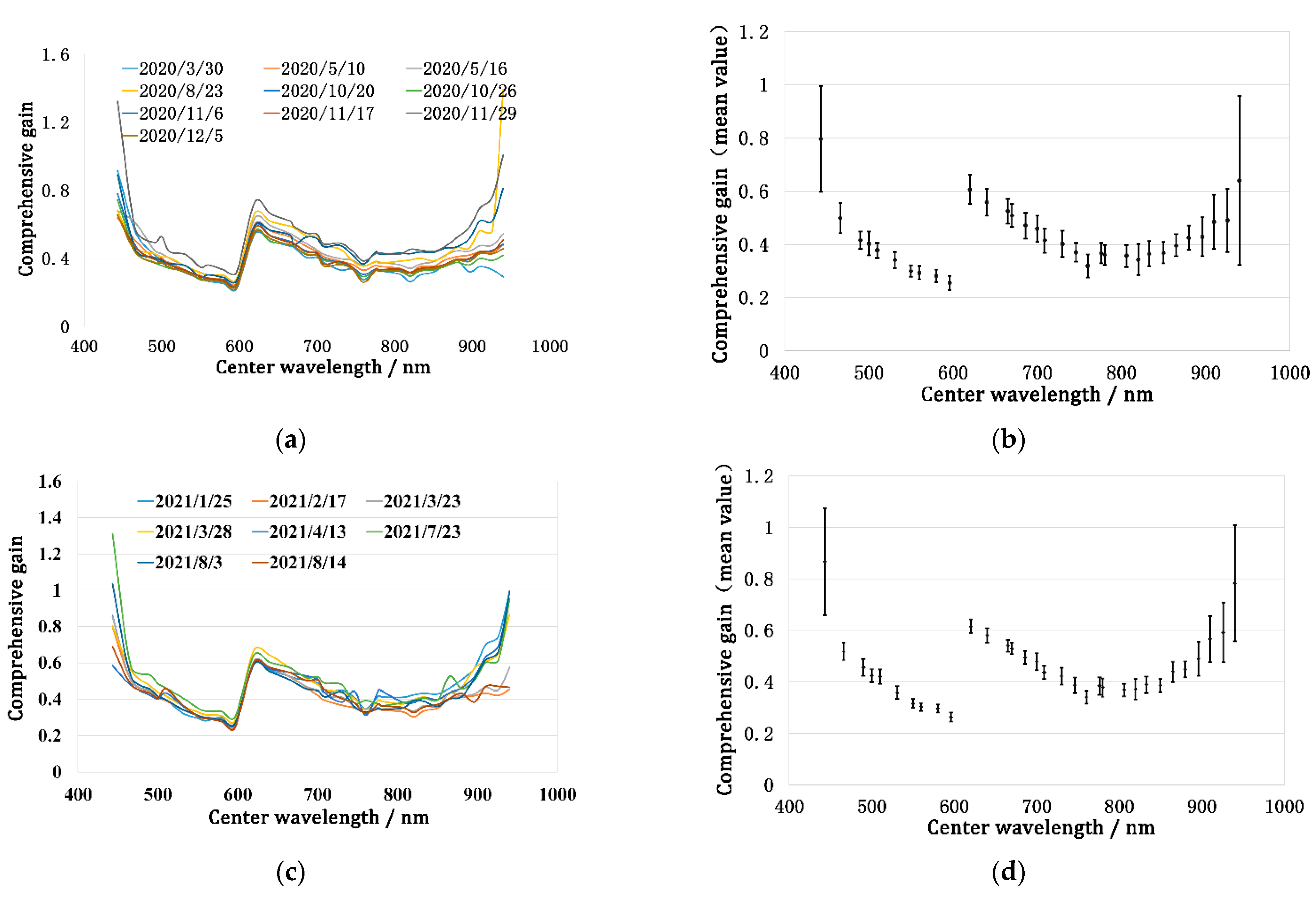
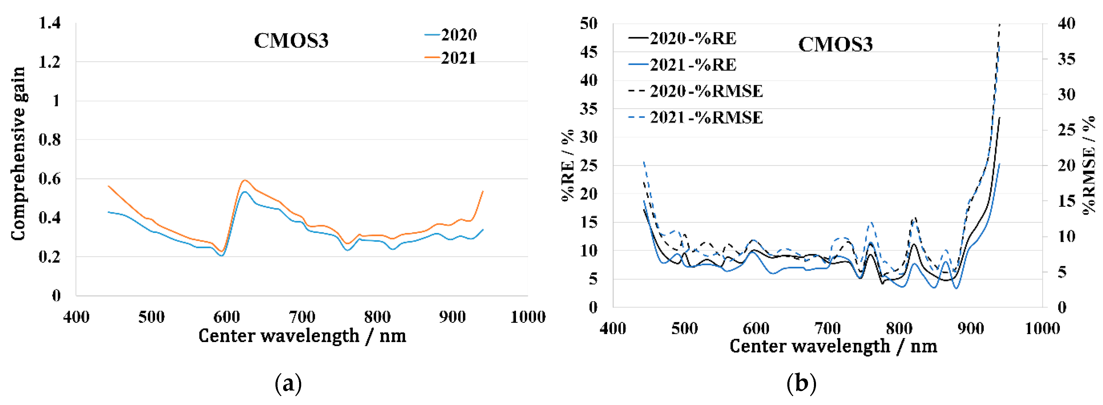
3.1.3. OHS-F CMOS3 Calibration Results and Analysis
3.2. Comprehensive Gain Calculation Results
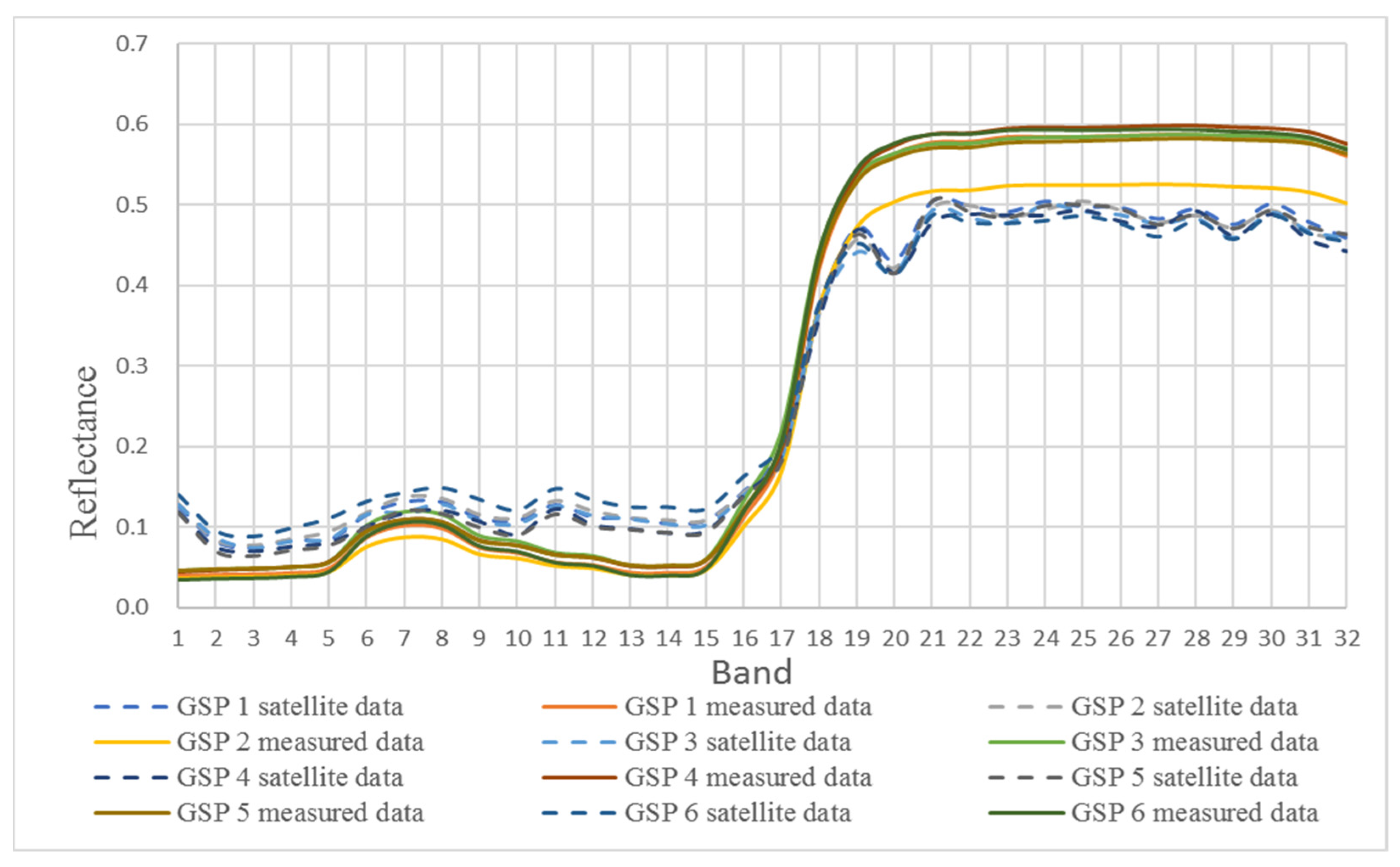
3.3. Validation Using the Ground Measured Reflectance
4. Discussion
5. Conclusions
- (1)
- The calibration model developed in this paper is suitable for use with hyperspectral sensors designed with gradient filters, which will be very helpful to the calibration of low-cost commercial micro-nano satellite constellations such as the “Zhuhai-1” satellite constellation.
- (2)
- The comprehensive gains in 2020 and 2021 calculated by using the calibration data for four sites of RadCalNet displayed good consistency, which shows the rationality of the comprehensive gain defined in this paper. Except for a few bands, the relative error of the calibration results in a single observation period was less than 10%.
- (3)
- The consistency of the calibration results for satellite sensors in 2021 was significantly higher than that in 2020, mainly due to the poor radiometric stability of satellite sensors in the early stage of the launch.
- (4)
- The overall trend in the comprehensive gain in 2020 and 2021 fitted by the least squares method was similar, which can reflect the change in the sensors’ radiation performance over time. Except for the individual gas absorption bands and low signal-to-noise ratio bands, the fitting error was below 10% during the calculation of the comprehensive gains.
- (5)
- The radiometric calibration results were applied to obtain the satellite reflectance data. Compared to the reflectance spectrum of cotton measured on the ground, the trend in the surface reflectance curve retrieved by the OHS-F satellite CMOS2 sensor was consistent.
Author Contributions
Funding
Data Availability Statement
Acknowledgments
Conflicts of Interest
References
- Wei, W. Research on Long Time Series Calibration Method of Satellite Remote Sensor Based on Global Calibration Site Network; University of Science and Technology of China: Hefei, China, 2017. [Google Scholar]
- Saunier, S.; Karakas, G.; Yalcin, I.; Done, F.; Mannan, R.; Albinet, C.; Goryl, P.; Kocaman, S. SkySat Data Quality Assessment within the EDAP Framework. Remote Sens. 2022, 14, 1646. [Google Scholar] [CrossRef]
- Xingfa, G. Principles and Methods of Radiometric Calibration of Aerospace Optical Remote Sensors; Science Press: Beijing, China, 2013. [Google Scholar]
- Wilson, N.; Greenberg, J.; Jumpasut, A.; Collison, A. In-Orbit Radiometric Calibration of the Planet Dove Constellation. 2017. Available online: https://digitalcommons.usu.edu/calcon/CALCON2017/All2017Content/23/ (accessed on 20 October 2017).
- Czapla-Myers, J.; Thome, K.; Wenny, B.; Anderson, N. Railroad Valley Radiometric Calibration Test Site (RadCaTS) as Part of a Global Radiometric Calibration Network (RadCalNet). In Proceedings of the IGARSS 2020—2020 IEEE International Geoscience and Remote Sensing Symposium, Waikoloa, HI, USA, 26 September–2 October 2020. [Google Scholar]
- Scanlon, T.; Greenwell, C.; Czapla-Myers, J.; Anderson, N.; Goodman, T.; Thome, K.; Wolliams, E.; Porrovecchio, G.; Linduška, P.; Šmíd, M.; et al. Ground comparisons at RadCalNet sites to determine the equivalence of sites within the network. In Proceedings of the SPIE Remote Sensing, Warsaw, Poland, 29 September 2017; Volume 10423, pp. 255–267. [Google Scholar]
- Jing, X.; Leigh, L.; Teixeira Pinto, C.; Helder, D. Evaluation of RadCalNet Output Data Using Landsat 7, Landsat 8, Sentinel 2A, and Sentinel 2B Sensors. Remote Sens. 2019, 11, 541. [Google Scholar] [CrossRef]
- Ma, L.; Zhao, Y.; Woolliams, E.R.; Dai, C.; Wang, N.; Liu, Y.; Li, L.; Wang, X.; Gao, C.; Li, C.; et al. Uncertainty analysis for RadCalNet instrumented test sites using the Baotou sites BTCN and BSCN as examples. Remote Sens. 2020, 12, 1696. [Google Scholar] [CrossRef]
- Shrestha, M.; Helder, D.; Christopherson, J. DLR Earth Sensing Imaging Spectrometer (DESIS) Level 1 Product Evaluation Using RadCalNet Measurements. Remote Sens. 2021, 13, 2420. [Google Scholar] [CrossRef]
- Bouvet, M.; Thome, K.; Berthelot, B.; Bialek, A.; Czapla-Myers, J.; Fox, N.P.; Goryl, P.; Henry, P.; Ma, L.; Marcq, S.; et al. RadCalNet: A radiometric calibration network for Earth observing imagers operating in the visible to shortwave infrared spectral range. Remote Sens. 2019, 11, 2401. [Google Scholar] [CrossRef]
- Wenny, B.N.; Thome, K.; Czapla-Myers, J. Evaluation of vicarious calibration for airborne sensors using RadCalNet. J. Appl. Remote Sens. 2021, 15, 034501. [Google Scholar] [CrossRef]
- Zhao, Y.; Ma, L.; Li, C.; Gao, C.; Wang, N.; Tang, L. Radiometric cross-calibration of Landsat-8/OLI and GF-1/PMS sensors using an instrumented sand site. IEEE J. Sel. Top. Appl. Earth Obs. Remote Sens. 2018, 11, 3822–3829. [Google Scholar] [CrossRef]
- Alhammoud, B.; Jackson, J.; Clerc, S.; Arias, M.; Bouzinac, C.; Gascon, F.; Cadau, E.G.; Iannone, R.Q.; Boccia, V. Sentinel-2 Level-1 Radiometry Assessment Using Vicarious Methods From DIMITRI Toolbox and Site Measurements From RadCalNet Database. IEEE J. Sel. Top. Appl. Earth Obs. Remote Sens. 2019, 12, 3470–3479. [Google Scholar] [CrossRef]
- Marcq, S.; Meygret, A.; Bouvet, M.; Fox, N.; Greenwell, C.; Scott, B.; Berthelot, B.; Besson, B.; Guilleminot, N.; Damiri, B. New Radcalnet Site at Gobabeb, Namibia: Installation of the Instrumentation and First Satellite Calibration Results. In Proceedings of the IGARSS 2018—2018 IEEE International Geoscience and Remote Sensing Symposium, Valencia, Spain, 22–27 July 2018. [Google Scholar]
- Gao, C.; Liu, Y.; Wu, Z.; Ma, L.; Qiu, S.; Li, C.; Zhao, Y.; Han, Q.; Zhao, E.; Qian, Y.; et al. An Approach for Evaluating Multisite Radiometry Calibration of Sentinel-2B/MSI Using RadCalNet Sites. IEEE J. Sel. Top. Appl. Earth Obs. Remote Sens. 2021, 14, 8473–8483. [Google Scholar] [CrossRef]
- Zhao, Y.; Ma, L.; Li, W.; He, H.; Long, X.; Wang, N.; Liu, Z.; Qian, Y.; Qiu, S.; Liu, Y.; et al. Vicarious Radiometric Calibration of Superview-1 Sensor Using RadCalNet TOA Reflectance Product. In Proceedings of the 2021 IEEE International Geoscience and Remote Sensing Symposium IGARSS, Brussels, Belgium, 11–16 July 2021; pp. 8130–8133. [Google Scholar]
- Li, W.; Ma, L.; Zhao, Y.; Liu, Y.; Wang, N.; Qian, Y.; Li, K.; Li, C.; Tang, L. Temporal Vicarious Radiometric Calibration of ZY-3 Mux Sensor Using Automatic Ground Measurement of Baotou Sandy Site in China. In Proceedings of the 2021 IEEE International Geoscience and Remote Sensing Symposium IGARSS, Brussels, Belgium, 11–16 July 2021; pp. 7767–7770. [Google Scholar]
- Vermote, E.F.; Tanré, D.; Deuze, J.L.; Herman, M.; Morcette, J.J. Second Simulation of the Satellite Signal in the Solar Spectrum, 6S: An overview. IEEE Trans. Geosci. Remote Sens. 1997, 35, 675–686. [Google Scholar] [CrossRef] [Green Version]


| Sensor Parameter | Value | |
|---|---|---|
| Satellite | Total satellite mass | 67 kg |
| Orbit height | 500 km | |
| Orbit inclination angle | 98° | |
| Regression cycle | 2.5 days | |
| Sensor | Field of view (FOV) | 20.5° |
| Signal-to-noise ratio (SNR) | ≥300 dB | |
| Number of active detectors | 5056 × 2968 | |
| Detector size | 4.25 μm × 4.25 μm | |
| Sensor technology | Spectral filter | |
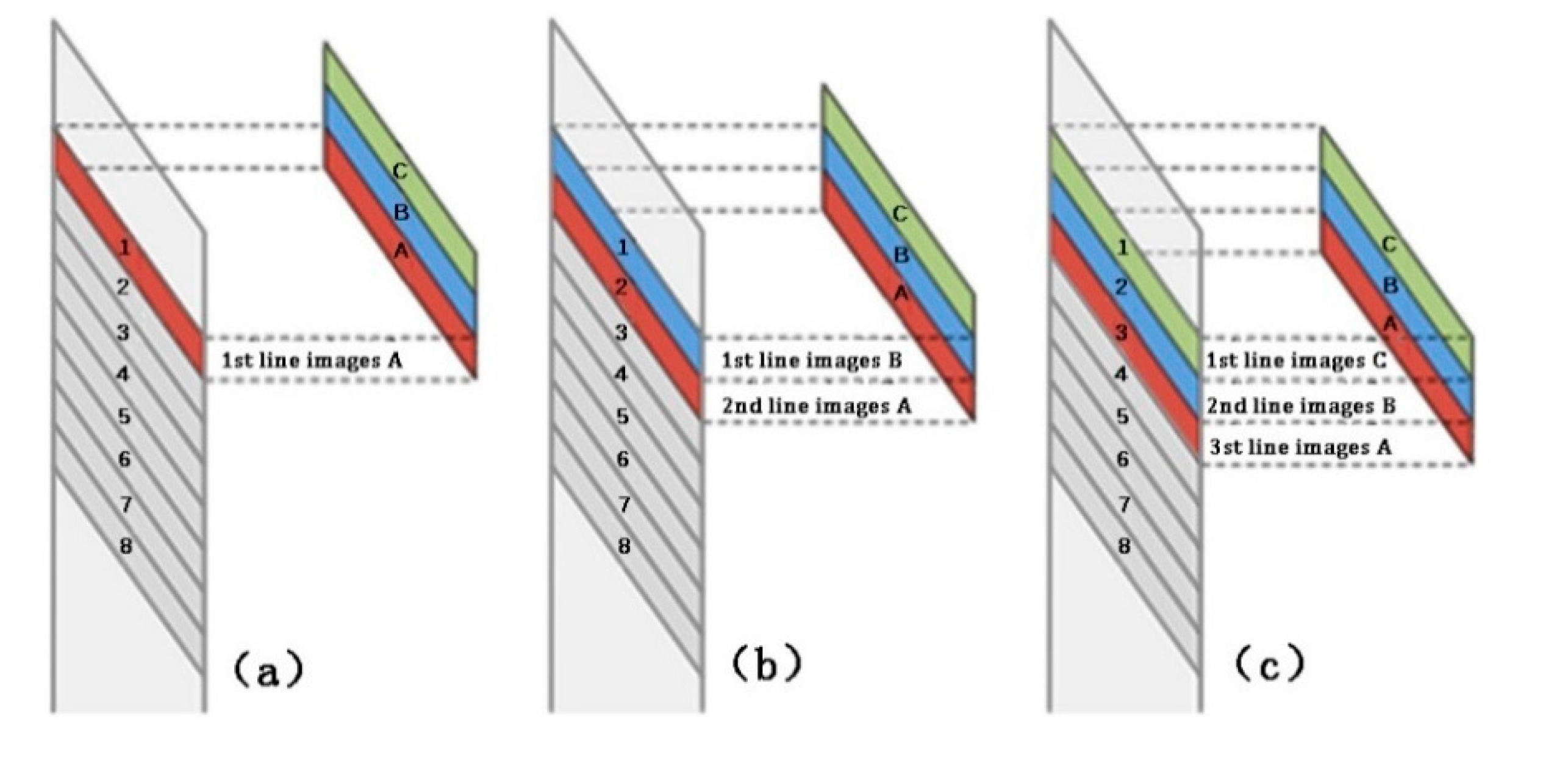
| Imaging mode | Push-broom imaging | |
| Resolution | 10 m | |
| Spectral range | 400 nm–1000 nm | |
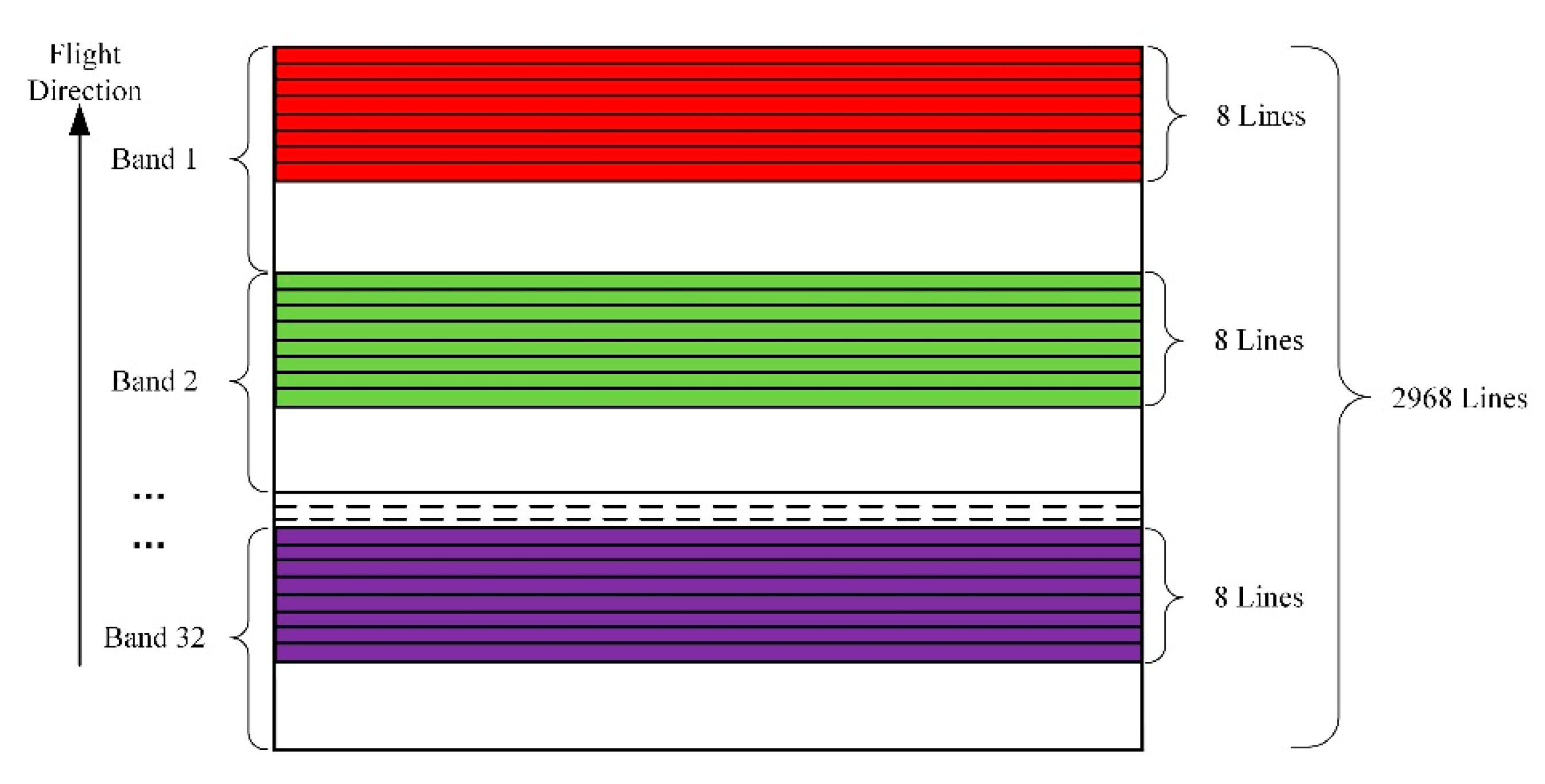
| Number of bands | 32 | |
| Quantization bits | 10 | |
| Width | 50 km × 3 |
| Filed | Abbr | Lon | Lat | DEM (km) | Type |
|---|---|---|---|---|---|
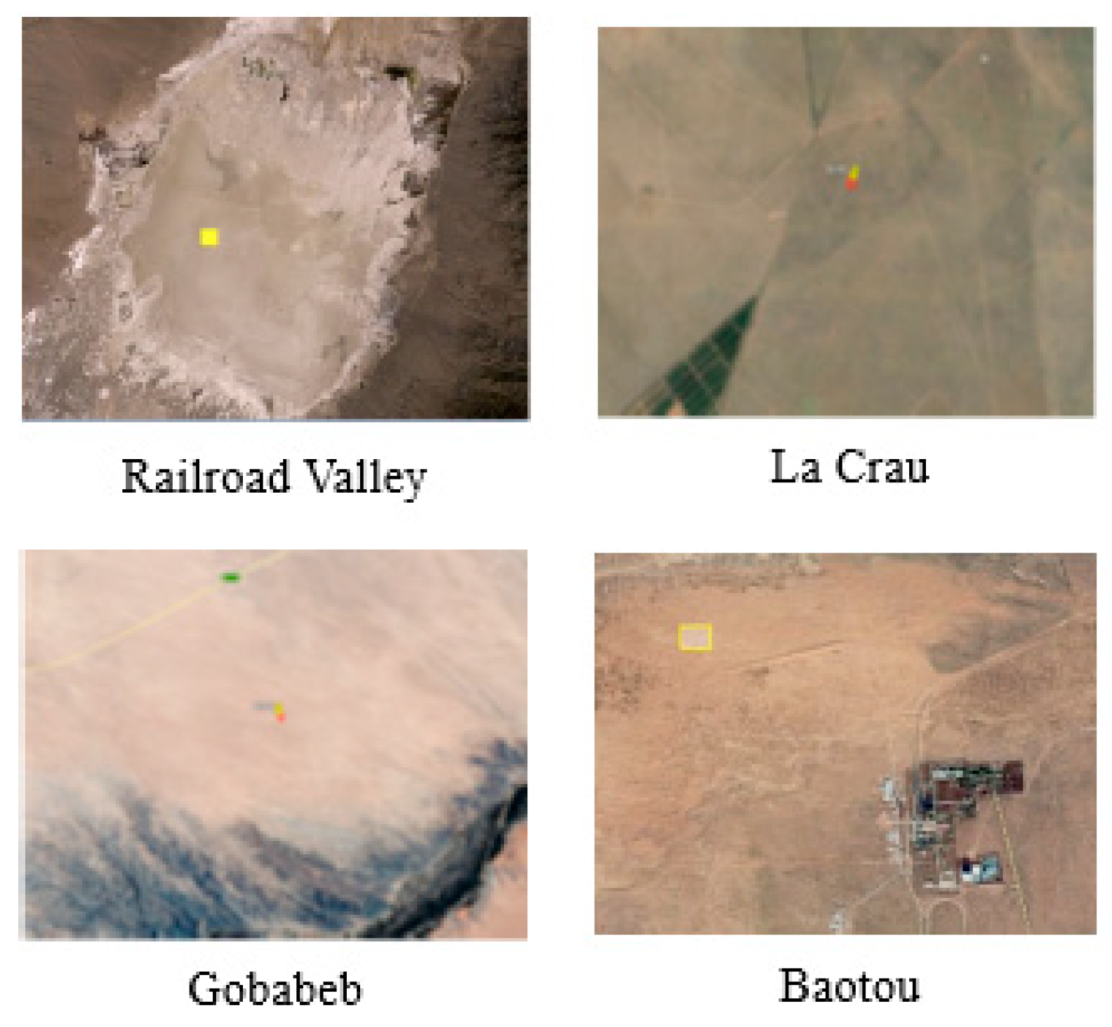
| Baotou, China | BTCN | 109.615° | 40.865° | 1.301 | desert |
| Gobabeb, Namibia | GBNA | 15.120° | −23.600° | 0.510 | desert |
| La Crau, France | LCFR | 4.860° | 43.559° | 0.020 | grassland and rock |
| Railroad Valley, United States | RVUS | −115.69° | 38.497° | 1.435 | desert |
| Date | Overpass Time (UTC) | AOD | WVC (g/cm2) | Ozone Content (atm-cm) |
|---|---|---|---|---|
| 5 April 2020 | 11:41:23 | 0.038 | 4.387 | 0.289 |
| 16 October 2020 | 5:54:45 | 0.073 | 0.005 | 0.280 |
| 24 November 2020 | 11:34:35 | 0.038 | 2.168 | 0.276 |
| 5 December 2020 | 20:55:12 | 0.018 | 0.128 | 0.260 |
| 22 December 2020 | 20:57:11 | 0.016 | 0.686 | 0.285 |
| 31 January 2021 | 20:53:12 | 0.025 | 0.441 | 0.305 |
| 6 March 2021 | 20:51:37 | 0.056 | 0.388 | 0.296 |
| 3 April 2021 | 20:53:09 | 0.043 | 0.366 | 0.296 |
| 12 May 2021 | 20:54:29 | 0.092 | 0.244 | 0.341 |
| 5 June 2021 | 5:52:40 | 0.077 | 0.508 | 0.331 |
| 9 June 2021 | 12:54:55 | 0.133 | 2.336 | 0.328 |
| 26 June 2021 | 11:31:11 | 0.071 | 1.969 | 0.273 |
| 7 July 2021 | 11:31:56 | 0.066 | 1.380 | 0.285 |
| 9 August 2021 | 11:32:32 | 0.109 | 1.519 | 0.277 |
Publisher’s Note: MDPI stays neutral with regard to jurisdictional claims in published maps and institutional affiliations. |
© 2022 by the authors. Licensee MDPI, Basel, Switzerland. This article is an open access article distributed under the terms and conditions of the Creative Commons Attribution (CC BY) license (https://creativecommons.org/licenses/by/4.0/).
Share and Cite
Zhang, Q.; Zhao, Y.; Zhang, L.; Wu, J.; Li, W.; Yan, J.; Jiang, X.; Yan, Z.; Zhao, J. On-Orbit Radiometric Calibration of Hyperspectral Sensors on Board Micro-Nano Satellite Constellation Based on RadCalNet Data. Remote Sens. 2022, 14, 4720. https://doi.org/10.3390/rs14194720
Zhang Q, Zhao Y, Zhang L, Wu J, Li W, Yan J, Jiang X, Yan Z, Zhao J. On-Orbit Radiometric Calibration of Hyperspectral Sensors on Board Micro-Nano Satellite Constellation Based on RadCalNet Data. Remote Sensing. 2022; 14(19):4720. https://doi.org/10.3390/rs14194720
Chicago/Turabian StyleZhang, Qiang, Yongguang Zhao, Lei Zhang, Jiaqi Wu, Wan Li, Jun Yan, Xiaohua Jiang, Zhiyu Yan, and Jing Zhao. 2022. "On-Orbit Radiometric Calibration of Hyperspectral Sensors on Board Micro-Nano Satellite Constellation Based on RadCalNet Data" Remote Sensing 14, no. 19: 4720. https://doi.org/10.3390/rs14194720