


Unsupervised Domain Adaptation with Adversarial Self-Training for Crop Classification Using Remote Sensing Images


1
Geoinformatic Engineering Research Institute, Inha University, Incheon 22212, Korea
2
Department of Geoinformatic Engineering, Inha University, Incheon 22212, Korea
*
Author to whom correspondence should be addressed.
Remote Sens. 2022, 14(18), 4639; https://doi.org/10.3390/rs14184639
Submission received: 11 August 2022
/
Revised: 13 September 2022
/
Accepted: 14 September 2022
/
Published: 16 September 2022
(This article belongs to the Special Issue Remote Sensing of Vegetation Biochemical and Biophysical Parameters)
Abstract
:Crop type mapping is regarded as an essential part of effective agricultural management. Automated crop type mapping using remote sensing images is preferred for the consistent monitoring of crop types. However, the main obstacle to generating annual crop type maps is the collection of sufficient training data for supervised classification. Classification based on unsupervised domain adaptation, which uses prior information from the source domain for target domain classification, can solve the impractical problem of collecting sufficient training data. This study presents self-training with domain adversarial network (STDAN), a novel unsupervised domain adaptation framework for crop type classification. The core purpose of STDAN is to combine adversarial training to alleviate spectral discrepancy problems with self-training to automatically generate new training data in the target domain using an existing thematic map or ground truth data. STDAN consists of three analysis stages: (1) initial classification using domain adversarial neural networks; (2) the self-training-based updating of training candidates using constraints specific to crop classification; and (3) the refinement of training candidates using iterative classification and final classification. The potential of STDAN was evaluated by conducting six experiments reflecting various domain discrepancy conditions in unmanned aerial vehicle images acquired at different regions and times. In most cases, the classification performance of STDAN was found to be compatible with the classification using training data collected from the target domain. In particular, the superiority of STDAN was shown to be prominent when the domain discrepancy was substantial. Based on these results, STDAN can be effectively applied to automated cross-domain crop type mapping without analyst intervention when prior information is available in the target domain.
1. Introduction
In recent years, crop price variations and food supply instability have frequently occurred due to several issues including various extreme weather conditions caused by climate changes [1,2]. To adequately address food security issues, the importance of the continuous monitoring and effective management of agricultural environments is much greater than in the past. For agricultural environment monitoring, crop type mapping, which identifies which crop types are grown in agricultural fields, is regarded as the most basic and essential task [3,4,5]. Remote sensing technology that can consistently monitor the Earth’s environment is known to be the most effective method for crop type mapping [6,7].
Crop type maps are mainly generated using the supervised classification of remote sensing images. Several aspects including selecting images with optimal spatial and temporal resolutions, classification methodologies, and collecting training samples should be appropriately considered to obtain accurate crop classification results from remote sensing images [5,7,8,9,10,11]. Regarding classification methodologies, advanced models ranging from machine learning to deep learning have been applied to classify single or multi-temporal remote sensing images [12,13,14]. However, such models usually require a large set of training data to determine the appropriate decision boundaries. Thus, training data play a crucial role in improving the accuracy of supervised classification [14,15,16].
Training data are commonly extracted from ground truth data collected by field surveys. Several field surveys are frequently required to investigate phenological crop changes over a specific period. Since field surveys need much time and cost as well as the prior knowledge of experts, collecting sufficient training data for crop classification is not always possible. Even though advanced classification models can be applied to crop classification, the classification performance may be degraded when not enough training data are available, which has led to several studies on classification with limited training data [17,18,19]. For example, officially available annual products such as the cropland data layer (CDL) provided by the National Agricultural Statistics Service (NASS) of the United States Department of Agriculture (USDA) [20] can be used as prior information to extract representative crop samples [8,21,22]. However, such annual classification products are not always available for most smallholder farms [13].
Despite the difficulty in collecting ground truth data, annual nationwide crop type maps should be prepared for long-term crop monitoring and agricultural management. Furthermore, yearly crop type maps should be produced at field levels in major crop cultivation areas to provide decision-supporting information for national food policies [2,6,14,23]. For crop type mapping in a target year or region for which no training data are available, one possible approach is to train a classifier using past crop labels obtained from the same region or other regions with similar crop types and then classify the target region [24,25]. However, when the characteristics of the images used for training the classifier are different from those of the images used for classification, the classification performance might be unsatisfactory. For these domain or spectral shift problems, the generalization capability of the classification model learned from training samples in different spatial and temporal domains may be significantly reduced when applied to the target year or region.
Domain adaptation (DA) has been proposed to solve such spectral shift or discrepancy problems between the source and target domains in the classification of remote sensing images [26]. Unsupervised DA (UDA), one of the types of transfer learning, is frequently employed to transfer a classification model learned using training samples available in a source domain to the classification of an image in a target domain with no available training samples [24,25,26,27,28,29,30]. Many statistical and machine learning-based UDA methods have been presented to design specific mapping functions between the source and target domains [26,31].
Inspired by success in image segmentation and classification, various deep learning models have been proposed to effectively adapt different data distributions between the source and target domains; these can be divided into two categories: adversarial training and self-training [32]. Adversarial training extracts domain-invariant features by adding a discriminator to the model. The domain adversarial neural network (DANN), proposed by Ganin et al. [33], utilizes a domain classifier as a discriminator and is regarded as the most representative adversarial training model. DANN has shown promise in remote sensing image classification [24,27,29,30].
The second deep learning-based UDA category is self-training. It iteratively extracts training candidate samples in the target domain and then utilizes the pseudo-labeled samples to fine-tune the classifier [32]. The critical component of self-training is to extract the informative training candidates and assign accurate class labels to them. Several deep learning models including generative adversarial networks [28], convolutional neural networks (CNNs) [34], and appearance adaptation networks [35] have proven their ability to improve the quality of pseudo-labels in semantic segmentation.
Despite the significant potential of UDA for supervised image classification, there remain challenging issues for crop classification using remote sensing images. Multi-temporal images are usually considered for classification, and the same crops are also cultivated in different regions. Thus, the domain discrepancy in various domains is more pronounced in remote sensing images used as inputs for classification. For example, the same crop types or objects in one image may show significantly different spectral responses in other images due to spectral shifts caused by different atmospheric conditions, illumination conditions, and sensor types. Such spectral shifts result in the misclassification of the same crop types and spectral confusion between individual crops with similar spectral responses, thereby leading to the poor classification performance of UDA [25,36,37]. Furthermore, the type of spectral shift associated with data distributions significantly affects the classification performance and even varies across the spatial and/or temporal domain. It is still difficult to effectively solve spectral shift problems when the data distributions of the source and target domains are too different [25]. Thus, a UDA method that is robust to spectral shifts regardless of varying degrees of spectral shifts should be developed for crop classification using remote sensing images. However, most previous studies have not conducted extensive experiments on various cross-spatial and temporal domain discrepancies.
From a methodological viewpoint, adversarial training focuses on alleviating spectral shift problems by extracting domain-invariant features to improve the classification accuracy. If a feature extractor is learned correctly, it is known that better performance in source domain image classification leads to improved accuracy in the target domain image classification [33]. However, the classification performance of adversarial training-based models is significantly affected by the type of spectral shift between domains [24,25]. Meanwhile, self-training is intended to improve the classification accuracy by extracting pseudo-labeled samples informative to the classification in the target domain. Self-training can alleviate the above-mentioned limitation of adversarial training by converting the domain adaptation-based classification task to the classification task in the target domain. Therefore, leveraging the respective advantages of adversarial training and self-training within an integrated UDA framework could significantly increase the classification accuracy. To the best of our knowledge, however, previous studies on UDA rarely combined the respective advantages of both adversarial training and self-training.
In UDA-based crop classification, classification accuracy is significantly affected by the use of different sensor types and the difference in reflectance due to changes in the sowing time and growth conditions in crop cultivation regions. Such various domain shift cases frequently encountered in crop classification have not been thoroughly considered to evaluate the performance of conventional UDA methods. Furthermore, when cases with no available training samples in the target domain are considered for UDA-based crop classification, prior information in the target domain such as past crop boundary maps can be a valuable source of information for classification without analyst intervention. Particularly, past crop maps can facilitate the extraction of informative training candidates for self-training. However, the specific procedure for using such additional information for crop classification has not yet been considered in UDA.
To address the above-mentioned limitations, this study proposes a novel UDA framework called self-training with domain adversarial network (STDAN) tailored to crop classification using remote sensing images. STDAN first applies adversarial training to solve domain shift problems and generate initial classification results in the target domain. Then, self-training is employed to assign pseudo-labels on unlabeled training data in the target domain. In particular, specific procedures that consider spatial contextual information within each crop field and past crop boundary maps as additional information are presented to extract more reliable and informative training data in the target domain in an iterative way. The potential of STDAN was demonstrated via crop classification experiments using unmanned aerial vehicle (UAV) images where various spatial, temporal, and spatiotemporal domain discrepancy cases were mainly considered.
2. Methods
STDAN aims to solve spectral shifts between images collected at different regions and times as well as to generate crop type maps without analyst intervention. To this end, STDAN employs adversarial training and self-training, respectively, to alleviate the first issue and automatically collect new training data at the target domain using past parcel boundary maps in the study area. Specific procedures for self-training are designed to extract more accurate and informative training data in the target domain, leading to improved classification accuracy.
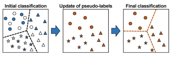
As illustrated in Figure 1, STDAN consists of three analysis stages: (1) DANN-based initial classification; (2) the self-training-based updating of training candidates using three specific constraints; and (3) the refinement of training candidates using iterative classification and final classification.
2.1. Stage 1: DANN-Based Initial Classification
When domain shifts between images acquired at different regions and times are significant, extracting the optimal domain-invariant features via conventional UDA approaches may not be feasible, making it difficult to obtain a satisfactory classification performance. This problem can be solved by switching the cross-domain classification task to a classification task in the target domain.
To this end, the first analysis stage of STDAN comprises an initial classification conducted using labeled training data in the source domain and unlabeled training data in the target domain, which is followed by the assignment of pseudo-labels to the unlabeled training data in the target domain. For this process, we employed DANN following the results of our previous study in which adversarial training-based DANN achieved superior prediction accuracy to other UDA methods including deep adaptation networks and deep reconstruction-classification networks [25].
DANN consists of three blocks: a feature extractor, a label classifier, and a domain classifier. As shown in Figure 2, the network combining the feature extractor and the label classifier is a kind of classifier with hierarchical convolutional structures. Only labeled training data in the source domain are usually used to train this classification network, focusing on the classification of source images. As a result, when the target image is classified using the classifier trained in the target domain, satisfactory performance may not be obtained due to the domain shift between cross-domain images. The domain classifier, which plays the most crucial role in DANN, is combined to solve this limitation. This classifier utilizes both the source domain and target domain training data as inputs and does not require the label information of the target image to be classified. To train this classifier, 0 and 1 (called domain labels) are assigned to the source and target domains, respectively.
The domain classifier, also called a discriminator, aims to learn domain labels that are indistinguishable from each other to make the feature distributions of the source and target images similar. This way of learning is achieved by applying a gradient reversal layer (GRL), which multiplies the loss value by a negative constant to change the sign and transfers it to the previous layer. The GRL is usually located in the top layer of the domain classifier. Since the label and domain classifiers share the parameters of the feature extractor, DANN can extract the domain-invariant features and achieve excellent generalization capability. Adversarial learning is performed by alternatively learning two separate networks. Initial classification in the target domain is then performed by only activating the feature extractor and the label classifier. Based on the initial classification result, pseudo-labels can be assigned to the unlabeled training candidates in the target domain.
2.2. Stage 2: Update of Training Candidates
Despite the excellent generalization capability of DANN, significant domain shifts may still degrade the prediction performance of target image classification. The poor classification performance will likely assign incorrect pseudo-labels to the initial training candidates in the target domain, accordingly, leading to poor classification accuracy in the target domain.
To address this issue, the second analysis stage considered three specific constraints on updating the initial training candidates that may have incorrect pseudo-labels. By sequentially applying the three constraints examining the correctness of the pseudo-labels, only training candidates with correct and confident pseudo-labels can be selected for further classification in the target domain. The three constraints mainly designed for crop classification are detailed as follows.
2.2.1. Confidence Information of DANN-Based Initial Classification
The first constraint requires the selection of pixels from the initial classification with more confidence (equivalently, less uncertainty). The assumption adopted in this study was that the initial training candidates likely to be classified incorrectly have a high uncertainty attached to the classification. The confidence information can be quantified from the stability in the class assignment during the training process of DANN.
In general, deep learning models are iteratively trained to determine the optimal hyperparameters and weights. As illustrated in Figure 3, training candidates located far away from the decision boundary in the feature space would be correctly classified, even with a small number of epochs. In contrast, any training candidate close to the decision boundary will likely have a high uncertainty, and many iterations are required to converge to the optimal hyperparameter. As a result, the pseudo-labels may differ for each epoch.
In this study, the confidence attached to the pseudo-labeling is defined as the proportion of the pseudo-label assigned to a specific class label during iterations. Let and be the class label determined from the DANN-based classification and the predicted class label at any pixel location x for the kth epoch, respectively. The degree of confidence denoted as is then defined as:
where K is the number of epochs, and is the indicator transform defined as:
After defining the degree of confidence at each pixel in the target domain image, a specific thresholding value should be set to extract more confident or less uncertain training candidates. However, if the thresholding is purely based on the confidence measure, most training candidates are likely to be selected only from specific parcels or certain crop types with high confidence, which violates the principle of independency and causes an imbalance problem [38].
Instead, we utilized an existing parcel boundary map in the study area to avoid such an imbalance problem. In general, the crop type grown in parcels may vary annually, but the shape of crop parcels remains unchanged, unless abrupt changes occur within the study area. Hence, the field survey data collected in the past can provide information on the crop boundaries. It should be noted that the crop types from field surveys are not used because they may vary annually.
In this study, the top 50% of pixels in the order of highest confidence were first extracted from individual fields and considered as training candidates. The training candidate pixels with a proportion value of less than 50% were excluded from the candidate set to collect more confident ones. Furthermore, the maximum pixel number was restricted to 50 per parcel to avoid the class imbalance problem. Once the thresholding values were predefined, this updating procedure based on confidence information could extract reliable training candidates representing individual parcels without analyst intervention.
2.2.2. Local Spatial Contextual Information
As land-cover types generally have spatial dependence, neighboring pixels are likely to have the same land-cover type [39]. Such spatial contextual information has been widely incorporated into spectral information for remote sensing image classification [40,41]. Along with the information on the degree of confidence, spatial contextual information can provide useful information to update the initial training candidates.
The second constraint for updating the initial training candidates requires the use of local spatial contextual information from the initial classification results. More specifically, this update process utilizes the initial DANN-based classification result in the target domain image and the training candidates refined by the first constraint. Whether or not the training candidate is updated is determined by the similarity between the pseudo-label of the initial training candidate pixel and the class labels of the surrounding pixels. If all pixels within a search neighborhood centered on the training candidate pixel have the same class label, the pseudo-label of the training candidate seems correct. Such pixels are regarded as confident training candidates.
Figure 4 illustrates an example of using local spatial contextual information for updating the training candidates. The class labels of eight pixels within the 3 by 3 search neighborhood were compared with that of the central training candidate pixel. In this example, only the training candidate pixel denoted as was accepted as the training pixel. Meanwhile, the two pixels denoted were rejected because the class labels within the search neighborhood were different. In this study, the search neighborhood size was set to be the same as the input patch size of DANN.
2.2.3. Representativeness of Pseudo-Labels in a Parcel Unit
As a single crop type is commonly grown in individual parcels, any pixel within a specific parcel will likely have the same class label. Even though training candidates are updated using the two constraints, training candidates within a specific crop parcel may still have different pseudo-labels. Thus, training candidates with different labels within the same crop parcel should be further updated.
The third constraint requires the consideration of the representativeness of pseudo-labels within individual parcels using the crop parcel boundary map as additional data. Only the training candidate pixels with the most frequent class label (hereafter referred to as the representative label) within each crop parcel were finally selected as representative training samples of the crop parcel. As shown in Figure 5, parcels A and D contained training candidates with different pseudo-labels, whereas all candidates within parcels B and C had the same pseudo-label. Only the candidate pixels with the representative pseudo-label (i.e., class 1) were selected for parcels A and D, whereas all the candidate pixels were selected for parcels B and C.
2.3. Stage 3: Iterative Refinement of Training Data and Final Classification
In stage 2, training candidates with the most confident pseudo-label were extracted by applying three constraints specific to crop classification. Even though more confident or reliable pixels have been selected, the accuracy of the pseudo-label assigned to the training candidates heavily depends on the performance of the DANN-based initial classification. The poor classification performance of the initial classification would lead to the incorrect allocation of crop types for training candidates. Possibly, some pixels with a higher degree of confidence may be misclassified. As a result, when the most frequent or representative pseudo-label selected within a certain crop parcel is incorrectly assigned, all the final training candidates selected by the third constraint accordingly had the incorrect label. This incorrect assignment may be due to the misclassification of spectrally ambiguous crops and the majority rule for selecting the representative pseudo-label. Thus, it is necessary to modify the class label incorrectly assigned by the majority rule and misclassification.
From a practical viewpoint, it is not feasible to judge the correctness of pseudo-labels, since no true label information is available in an unsupervised learning approach. As an alternative, the following reasonable assumption was adopted: reclassification using confident training candidates selected from stage 2 can return more reliable classification results than the initial classification results. Hence, a comparison of the pseudo-labels predicted from reclassification with the representative pseudo-labels assigned to individual parcels can facilitate finding parcels with incorrect representative pseudo-labels.
In stage 3, self-training-based iterative classification is employed to refine the possibly incorrect representative pseudo-label assigned to training candidates in the parcel unit. The refined training data are then used as final training data for classifying the target domain image.
The analysis in stage 3 begins by finding any crop parcel with training candidates assigned to the pseudo-label different from the actual one. The training candidates updated in stage 2 are first divided into training and validation samples for learning a new classification model and evaluating the prediction performance of the trained new classification model, respectively. When there are several crop parcels with the same representative class, training candidates in one crop parcel are used as validation pixels, and the ones in the remaining other parcels are used as training samples. This partitioning is implemented through a random selection.
The reliability of the initial representative pseudo-label is determined by a comparison with the predicted label from reclassification. The pseudo-label is kept unchanged when reclassification returns the same class label as the representative pseudo-label of the validation parcel. In contrast, if the class label different from the representative pseudo-label is obtained from reclassification, the representative pseudo-label is considered incorrect. The representative pseudo-label is then changed to the class label from reclassification, under the assumption that the reliability of the reclassification results is much better than that of the initial classification results.
This procedure is illustrated in Figure 6. Suppose the training candidates in B2 and B6 parcels, of which the actual label is B, are selected as validation samples for the first reclassification. Given that the pseudo-labels of the B2 and B6 parcels are assigned to B and A, respectively, it can be considered that the representative pseudo-label of the B6 parcel is incorrectly assigned through stage 2. Therefore, by using the training candidates with the class information via reclassification, the pseudo-label of the B6 parcel should be changed to B. In this study, the predicted class label by reclassification was assumed to be the actual representative label that is unavailable. The training candidates with the modified representative pseudo-labels are then used for the subsequent reclassification. The final training data determined through these repeated classifications are used to produce the classification result in the target domain.
The above-mentioned refinement procedure is iteratively applied to all parcels in the study area. It requires a lot of computational cost as the number of parcels searched in the study area increases. Thus, the iterative process of selecting validation parcels is repeated until a predefined stopping condition. If the pseudo-label of any training candidate is not updated until iterative reclassification corresponding to the number of parcels with major crops, it is assumed that all training candidates have already been updated, and the iterative classification is terminated. Preliminary experiments have confirmed that this stopping condition is appropriate for finding training candidates with incorrect pseudo-labels, even without examining all of the possible searching cases.
Iterative classification for training data refinement also requires heavy computational loads. The prediction accuracy of supervised classification using enough reliable training data is not significantly affected by model complexity [42,43]. STDAN can collect high-quality training data representing all classes in a target domain image through three-stage training candidate extraction and refinement processes. Therefore, a model with the same structures and hyperparameters as the DANN’s label predictor can be employed for iterative classification.
3. Experiments
3.1. Study Areas
The classification performance of STDAN was evaluated via extensive crop classification experiments in two agricultural areas including sub-areas in the Gangwon and Gyeongsang Provinces, Korea (Figure 7a).
The first case study area was Anbandegi, located in the Gangwon Province, one of the major highland Kimchi cabbage cultivation regions in Korea (hereafter referred to as Gangwon). In the study area, cabbage and potato are grown together and some parcels are managed as fallow to prevent crop pests [6]. All crops are planted and harvested from June to September, but there is an interval of about two weeks to one month between the sowing and harvesting times for each crop [14]. The average size of the crop parcels in Gangwon is about 0.6 ha.
The second case study area, in which garlic and onion are mainly grown, includes Hapcheon and Changyoeung in Gyeongsang Province (hereafter referred to as Gyeongsang). There are some barley and fallow parcels as well as garlic and onion in the study area. Unlike Gangwon, where each crop has different sowing and harvesting times, all crops in Gyeongsang are planted in November and harvested in late May. Garlic and onions are mulched after sowing until mid-March, and their vitality peaks in late April. Accordingly, images acquired from late March to early May were used for classification. The average size of the crop parcels in Gyeongsang is about 0.24 ha, which is relatively small compared with that of Gangwon (0.6 ha).
3.2. Datasets
UAV images were used as inputs for crop classification considering the size of the individual crop parcels and the short growing period of crops in the two study areas. The preprocessed UAV mosaic images with a spatial resolution of 50 cm were provided by the National Institute of Agricultural Sciences (NAAS). The UAV images were acquired by a fixed-wing eBee (senseFly, Cheseaux-sur-Lausanne, Switzerland) equipped with an RGB camera (IXUS/ELPH camera, Canon, Melville, NY, USA), and by a rotary-wing Matrice 200 (DJI, New Territories, Hong Kong) equipped with a five-band multispectral camera including the red, green, blue, red-edge, and near-infrared channels (RedEdge-MX, MicaSense, Seattle, WA, USA). Several preprocessing steps for the raw UAV images including orthorectification and relative radiometric correction were performed using Pix4Dmapper (Pix4D S.A., Prilly, Switzerland). Finally, three visible channels were used for supervised classification based on our preliminary study in the study areas [14,25].
Considering the different cultivation environments and growth cycles of crops between the two study areas, three multi-temporal UAV images and a single-date image were considered for crop classification in Gangwon and Gyeongsang, respectively (Table 1). It should be noted that UAV image acquisition was not performed annually in the two study areas, and not all of the acquired images were of good quality. Hence, the different image combinations were determined by considering the number of images available for the study areas. Detailed explanations of the optimal image combinations can be found in Kwak et al. [14,25].
Individual crops in the two study areas have distinct phenological growth patterns. However, their sowing and harvesting times can vary slightly, depending on the region and year. For example, a specific crop type grown in one year may be changed to another crop type or fallow in another year. Hence, images acquired in differing years or in another region inevitably cause domain discrepancy problems, resulting in spectral shifts in the images.
To investigate the effects of various domain discrepancy cases across spatial and temporal domains on classification accuracy, some sub-areas in Gangwon and Gyeongsang were selected for crop classification experiments (Figure 7b and Table 1). The sub-areas of Gangwon include the central part of Anbandegi (CA) and the northern part of Anbandegi (NA). Three sub-areas—Hapcheon Yaro (HY), Hapcheon Chogye (HC), and Changnyeong Yueo (CY)—were considered for Gyeongsang. To define the temporal domain discrepancy case in consideration of the data availability, UAV images acquired in multiple years were used mainly for CA and HC.
Ground truth data collected by field surveys and the visual inspection of UAV images were provided by the NAAS. The training and test data were extracted from the ground truth data and used for model training and accuracy evaluation, respectively. The ground truth data were also used to mask non-crop areas in the study areas. In addition, parcel boundary information was extracted from the ground truth data and used to update and refine training candidates in stages 2 and 3, respectively, in STDAN.
3.3. Design of Domain Adaptation Cases
To evaluate the potential of STDAN for UDA-based crop classification tasks, six domain adaptation cases were designed depending on the availability of UAV images acquired in the two study areas (Table 2). In this regard, three DA tasks were first designed: temporal, spatial, and spatiotemporal adaptation tasks. The temporal and spatial adaptation tasks are intended to solve domain shifts between the source and target caused by different UAV image acquisition regions and locations, respectively. The spatiotemporal adaptation task deals with spectral shift problems due to both temporal and spatial inconsistency.
3.4. Training and Test Data Sampling
STDAN aims to achieve UDA-based crop classification without analyst intervention. Although training data in the target domain is required for STDAN, prior information in the source domain should also be collected to guide the learning process for the classification in the target domain. This study assumes that ground truth data collected from previous years or other regions are already available in the target domain. In this study, the training data in the source domain and the unlabeled training data in the target domain were collected for the six UDA cases described in Table 2. Here, the proportion of training samples between classes was determined using the parcel areas for each crop type in the study areas. The unlabeled training data in the target domain were selected via random extraction from the UAV images without considering the proportion of the training samples between classes because the ground truth data in the target domain were assumed to be unavailable. From the preliminary test, random extraction could reasonably reproduce the proportion of training samples similar to the parcel areas. Ultimately, 5000 labeled training data in the source domain and 5000 unlabeled training data in the target domain were finally collected for the two study areas. All of the pixels in the target images that did not overlap the training data were used as test data.
As STDAN employs CNNs as a classifier, the labeled training data were prepared in the patch unit [44]. Different training patches were collected at locations separated by the input patch size to avoid overlap between the image patches. In addition, the training patches were extracted to contain only image information within the crop parcel to minimize the impact of non-crop areas on the classification.
3.5. Optimization of DANN Model Parameters
To apply the DANN model in the first stage of STDAN, the optimal model structure and hyperparameters must be determined to ensure excellent adaptation capabilities. Since DANN only utilizes unlabeled training data in the target domain, validation data for the label classifier are unavailable. As an alternative, determining the optimal hyperparameters for DANN was replaced by verifying the classification performance in the source domain. For the validation of the DANN model, the labeled training data in the source domain were divided into two groups via random sampling: 80% for model training and 20% for model validation. Once the optimal model structure and hyperparameters were determined, the entire training data were used for model training.
The main hyperparameters of DANN are the input patch size, convolution filter size, numbers of hidden layers and neurons in each layer, dropout, optimizer, and learning rates. As many hyperparameters need to be determined, some hyperparameters already tuned or recommended in previous studies were used in this study. When the input patch size is small, a model is more likely to overfit [45]. On the other hand, using the large input patch may produce over-smoothed classification results [46]. Based on our previous study results [14,47], the input patch size and the convolution filter size were set to 9 × 9 and 3 × 3, respectively, to avoid over-smoothing. A rectified linear unit (ReLU) was applied as an activation function for all of the used layers. As an exception, a softmax function with four (the number of labels for crop types) and two (two domain labels) filters was used as the activation function for the last layers of the label classifier and the domain classifier, respectively. Both classifiers utilized a categorical cross-entropy loss function and were learned in an adversarial way by minimizing and maximizing each loss.
Two regularization strategies, early stopping and dropout regularization [14], were also applied to avoid overfitting during the model training. The early stopping strategy stops training at a specified epoch when model performance is no longer improving during training. Dropout regularization can reduce the inter-dependent learning among neurons by randomly dropping specific neurons during training.
Table 3 lists the hyperparameters tested in this study and the optimal hyperparameters determined through experiments.
3.6. Evaluation Procedures and Metrics
The Jeffries–Matusita (JM) distance was used to quantitatively measure the degree of spectral shifts between two domains. Previous studies showed that the JM distance is an accurate separability measure [48]. The JM distance ranges between 0 and 2. The closer the JM distance value is to 0, the smaller the distribution difference between the two domains. The JM distance values calculated using all of the training data were used as auxiliary information to compare the classification results.
For the evaluation criteria of the classification performance of STDAN, this study adopted two criteria: (1) the comparison with the source and target baselines and (2) the comparison of variations in the classification accuracy for the individual stages of STDAN. Since STDAN was proposed to improve the performance of UDA without training data in the target domain, the classification accuracy of STDAN was first compared with the source and target baselines. The source baseline is the application of a shallow CNN model trained on labeled training data in the source domain to classify the target image. The source baseline does not include any representation learning procedure to alleviate the spectral shift problem by extracting domain-invariant features in the source baseline. The target baseline uses the labeled training data in the target domain to train the shallow CNN model. For a fair comparison, learning for the target baseline utilized the training data generated by assigning the label information from the ground truth data to the unlabeled training data used for DANN. The prediction target for the target baseline is the same as for the source baseline. The CNN models used for the two baselines had the same architecture as the label classifier of DANN. When recalling the main objective of UDA, the prediction performance of DANN should be better than the source baseline (lower bound value) and similar to the target baseline (upper bound value). This evaluation criterion has been widely adopted in previous UDA studies [24,27,29,49].
The effectiveness of the three analysis stages included in STDAN was also assessed by examining the classification accuracy variations per individual stage. For the comparison of the initial, intermediate, and final classification results, three results were compared: the applications of (1) only stage 1, (2) stages 1 and 2 (denoted as STDAN2), and (3) all three stages (denoted as STDAN3). As the consideration of only stage 1 corresponds to the application of DANN, the first case is hereafter denoted as DANN.
The quantitative classification performance of all classifiers—comprising the source baseline, the target baseline, DANN, and STDAN—was evaluated using the overall accuracy (OA) and F-measure. The F-measure, the harmonic mean of the user’s accuracy and producer’s accuracy [4], was used as a quantitative class-wise accuracy measure
3.7. Implementation
All of the procedures for classification and evaluation were implemented using programming with Python 3.6.7. DANN and CNN included within the STDAN framework were implemented using the TensorFlow [50] and Keras [51] libraries on Python 3.6.7. All classification models were run on the CentOS 7.0 operation system with an Intel XEON E5–2630 v4 @ 2.2GHz CPU and two NVIDIA RTX 3090 GPU with 24 GB of memory.
4. Results
4.1. Domain Shift Analysis Results
Prior to the crop classification experiments, this study first analyzed three factors affecting the domain discrepancy problems; the differences in (1) the proportions of crop parcels, (2) the crop growth conditions, and (3) sensor types. This analysis was performed because each domain discrepancy case described in Table 2 was affected by different factors.
The difference in the proportion between crops included in the source and target images was considered the first domain discrepancy factor and computed using ground truth data available in the two study areas. Figure 8 shows the difference in the proportion of individual crop parcels for some DA cases defined in Table 2. Different proportions of crop parcels between the source and target domains were observed for cases 2, 3, 5, and 6, mainly when different spatial domains were considered. In particular, as in cases 3 and 6, certain minor crops (potato and barley) present in the source image did not exist in the target image. In these cases, the proportions of crop parcels between the two domains considerably differed. There were no crop types that were not included in the source image, but existed in the target image.
As for the second domain discrepancy factor, different crop growth conditions between the two domains were considered in this study. The growth conditions or status of crops may vary depending on the weather conditions and crop pests in the study area. For example, case 5 in Figure 9 shows the difference in the growth status of crops between the source and target images. Garlic, onion, and barley could be easily identified in the source image. In contrast, plastic mulching was observed in some parcels, and garlic and onion in the center were not visually distinguishable in the target image due to their poor growth status. In addition, sowing and harvesting times may change for different years and regions. For cases 1 and 3 in Figure 8, highland Kimchi cabbage and potato showed different growth conditions in each parcel due to different sowing times.
The difference in the sensor types or image acquisition systems was also considered as the domain discrepancy factor (see Table 1). Even when images with the same RGB channel were used, as in case 2, the spectral wavelength ranges may differ, which makes DA tasks more difficult for crops with similar spectral characteristics.
Table 4 summarizes the influence degree of three factors on the domain discrepancy for all DA cases. The effect of the domain shifts was relatively small in the temporal adaptation, except for case 2, where different camera sensors were used. In contrast, the first two factors were more influential than the third one for the spatial and spatiotemporal adaptation cases.
The degrees of domain shifts were quantified using the JM distance (Table 5). Cases 1 and 4, which had few domain discrepancy factors, had relatively low JM distances compared with the other cases, corresponding to a case with minor changes in the physical conditions of individual crops between the two domains. Cases 3 and 6, with significant differences in the proportions of crop parcels and the crop growth conditions, also showed low JM distance values. As the difference in the sowing times of specific crops was observed only in some parcels, the domain discrepancy was not fully reflected in the JM distance value. On the other hand, case 2, with different camera sensors and case 5 with poor growth status, had relatively higher JM distance values than the other four cases. Consequently, satisfactory classification performance may not have been achieved for cases 2 and 5 with relatively large JM distance values, even though DANN was applied, due to the significant difference in the data distributions between the source and target domains. Thus, this case can be considered as an appropriate one to evaluate the classification performance of STDAN.
4.2. Visual Assessment of Classification Results
Figure 10 and Figure 11 compare the classification results for individual stages of STDAN with those of the source and target baselines as well as the ground truth data for the two study areas. The visual comparison results are detailed as follows.
4.2.1. Stage 1: DANN Results
DANN was applied in the first stage of STDAN to generate the initial classification results. In the classification results of cases 1, 3, 4, and 6 with relatively low JM distances, the source baseline result included misclassifications for some cases. The potato was misclassified as other crops in the source baseline result for case 1 in Gangwon due to the difference in the sowing times, as shown in the target image in Figure 9. The garlic and onion in Gyeongsang were misclassified as fallow near the parcel boundaries due to the significant difference in the proportions of fallow between the source and target domains (see Figure 8). DANN significantly improved such misclassification; therefore, the DA method should be applied to solve the domain shift problems between two images.
In the source baseline results for cases 2 and 5 with relatively high JM distances, most crop parcels were classified as a specific crop type, cabbage and onion for Gangwon and Gyeongsang, respectively (Figure 10 and Figure 11). Fallow parcels with distinct spectral properties were well-classified for both cases. These results indicate that crops with similar spectral responses are significantly affected by domain shifts. DANN significantly reduced the confusion between crop types for cases 2 and 5.
Despite the improved performance of DANN, its misclassification was more substantial than the source baseline for case 3, where the target image with different sowing times of specific crops was classified. Significant improvements in the classification performance of DANN were not observed for cases 2 and 5 compared with the cases with relatively low JM distance values. Furthermore, the DANN classification results exhibited misclassification near the parcel boundaries and isolated pixels. These visual inspection results indicate that DANN does not always guarantee superior classification performance to the source baseline.
4.2.2. Stage 2: Intermediate Classification Results of STDAN (STDAN2)
STDAN2, the intermediate classification applied up to stage 2, significantly reduced the misclassification at the parcel boundaries and isolated pixels in DANN. Park and Park [47] reported that these misclassifications were obtained when the training data for the CNN-based classification were mainly collected at the parcel boundaries. The application of the second criterion in stage 2 (i.e., using local spatial contextual information) could contribute to reducing the isolated pixels and updating the training candidates near the parcel boundaries. Furthermore, the misclassification of DANN in cases 2, 3, 4, and 5 was significantly improved by applying the third criterion in stage 2 (i.e., using the representative pseudo-label of individual parcels).
For cases 1, 3, 4, and 6 with low JM distances, the classification results of STDAN2 were significantly similar to that of the target baseline. As a low JM distance indicates significant similarity between two domains, no misclassification of most or all of the pixels within individual parcels was observed. Thus, the application up to stage 2 of STDAN could yield satisfactory classification results. Although STDAN2 exhibited better classification results compared with DANN for cases 2 and 5, some parcels were still misclassified. Therefore, the classification results for cases 2 and 5 demonstrate the necessity of applying stage 3 (i.e., the iterative refinement of training candidates) in STDAN.
4.2.3. Stage 3: Final Classification Results (STDAN3)
For cases 1, 3, 4, and 6 with a high similarity between the two domains, STDAN3 obtained via the application of stage 3 improved the misclassification of the parcel unit that could not be updated in stage 2. Additionally, misclassification was significantly improved by STDAN3 for cases 2 and 5 with considerable domain discrepancies. In case 2, most of the misclassified pixels in the eastern highland Kimchi cabbage parcels and the northern cabbage parcels were correctly classified in the STDAN3 results. Misclassification in the western onion parcels and the northern fallow parcel in STDAN2 for case 5 was also reduced in the STDAN3 results. The three-stage approach of STDAN could solve the misclassification problems in the parcel unit by modifying the incorrectly assigned pseudo-labels of training candidates through iterative reclassification.
4.3. Quantitative Accuracy Assessment Results
Figure 12 shows the OA values of five classification results: the source baseline, the target baseline, and three step-by-step classification results of STDAN. The classification accuracy of the source baseline was affected by the degree of domain discrepancy. The source baseline exhibited a low classification accuracy for cases 2 and 5, with significant differences between the two domains (the large JM distances in Table 5). As an exception, the accuracy of the source baseline for case 6 was very low, even though the JM distance value was the lowest among the six cases. Thus, misclassification in the source baseline may occur regardless of the domain discrepancy factors.
DANN significantly improved the classification accuracy for cases 2, 5, and 6 compared with the source baseline (27.95%p, 16.16%p, and 8.26%p, respectively). However, DANN did not perform satisfactorily for cases 2 and 5 compared with the other cases and STDAN results, despite the improved accuracy of DANN. The classification accuracy for cases 3 and 4 decreased by 5.85%p and 2.15%p, respectively, compared with the source baseline. As DANN could not fully solve the domain discrepancy problems, these results emphasize the necessity of STDAN for cross-domain classification.
STDAN2 and STDAN3 yielded gradual improvements in the classification accuracy compared with DANN for most cases. Improvements in classification accuracy were the most significant in cases 2 and 5, where the differences in the data distribution between the source and target domains were substantial. STDAN3 increased the classification accuracy by 12.28%p and 6.02%p for cases 2 and 5, respectively, compared with DANN.
Moreover, STDAN3 showed a classification accuracy compatible with the target baseline in the remaining cases, except for case 5. Therefore, these quantitative assessment results confirmed that STDAN is an effective UDA method for various domain discrepancy cases.
Figure 13 and Figure 14 show the F-measure of each crop type for all classification results. In cases 1, 3, and 4, where the variations in OA were not significant for the classifier, the accuracy of the major crop type in the two study areas did not drastically change. The accuracy of the minor crops and fallow showed some variations; however, these variations did not significantly influence the OA value due to their small proportions in the study areas.
For case 2, where a significant difference in OA was observed, the F-measure values of the source baseline for all classes, except for fallow, were significantly low. In particular, most of the potato pixels were misclassified. This poor accuracy of the source baseline was significantly improved by DANN. STDAN improved the decreased accuracy of fallow by DANN.
The confusion between garlic and barley was substantial in the source baseline result for case 5. Such confusion was also observed in case 4. Some barley were misclassified as garlic due to the similar spectral responses of barley and garlic, as reported in a previous study [14]. The misclassification resulting from the similar spectral properties of individual crops was gradually improved by the step-by-step application of STDAN.
What is noteworthy in case 6 is the significant decrease in the F-measure for fallow in the STDAN results. This poor classification accuracy of STDAN may have been due to the change in the proportions of fallow, the first domain discrepancy factor defined in this study. The fallow parcels occupy only 2.5% of the study area. The small proportions of fallow parcels may have resulted in the incorrect assignment of the representative pseudo-label in the parcel unit during the iterative reclassification in stage 3. However, the small occupancy of the fallow parcels did not result in a significant change in OA.
In summary, STDAN achieved the best classification performance that was robust to various domain discrepancy cases by improving the F-measure for all classes compared with the source baseline and DANN.
5. Discussion
5.1. Novelty of STDAN
Remote sensing images acquired at different atmospheric conditions and by different sensor types inevitably contain various domain shifts [26,52]. Tong et al. [34] reported that the performance of UDA considerably deteriorates when the spectral responses between classes are too similar or the number of classes increases.
To comprehensively examine these issues, this study considered three representative domain discrepancy factors frequently encountered in the classification of crops with similar spectral characteristics, as shown in Table 4. Moreover, the degree of the domain discrepancy per DA case was quantified using the JM distance (Table 5). According to the experimental results, various domain discrepancy problems make directly applying DANN to UDA tasks challenging. For example, DANN yielded relatively poor classification performance for cases 2 and 5, with significant domain differences. Furthermore, the classification accuracy of DANN was poorer than that of the source baseline due to the confusion between crops caused by varying sowing dates and similar spectral responses.
Previous UDA studies have generally focused on developing optimal deep learning models [28,30,35]. The end-to-end learning approach of deep learning models has the advantage of minimizing analyst intervention; however, it is challenging to reflect the characteristics of crops appearing in remote sensing images in the general deep learning model. As for an advanced UDA framework, STDAN was found to be robust to various domain shift cases. STDAN combines adversarial training and self-training to alleviate spectral shifts and extract informative training candidates without analyst intervention in the target domain, respectively. The novelty of STDAN lies in designing the three-stage approach tailored to UDA tasks for crop classification. In the first analysis stage of STDAN, DANN is employed to solve the domain inconsistency problems, and the DANN results are fed into the next self-training stage. If the initial training candidates generated from DANN inevitably include incorrectly assigned pseudo-labels, conventional self-training (where new informative training candidates are added to the new training data in the target domain) may fail to correctly solve error propagation problems caused by the training candidates with incorrect pseudo-labels [53].
To minimize the impact of such misclassification during self-training, the second and third stages in STDAN focus on excluding erroneous training candidates or modifying the incorrectly assigned pseudo-labels rather than adding new training samples using iterative classifications. In this regard, three constraints associated with the characteristics of the parcel-unit crop cultivation were presented in stage 2. The further refinement of pseudo-labels was implemented in stage 3 to extract more reliable training samples in the target domain. The poor classification performance of DANN for cases 2 and 5 with considerable domain shift problems indicates that many initial training candidates extracted from DANN may have erroneous pseudo-labels. The increased classification accuracy from the intermediate to the final classification confirms the effectiveness of individual stages employed in STDAN for various domain discrepancy cases.
Stages 2 and 3 can be regarded as the post-processing procedures used to alleviate the error propagation problems of DANN, which ensures the extensibility and applicability of DANN for crop classification. Once the DANN model for a specific DA task has been learned using sufficient information available in the source domain, the pre-trained DANN model can be directly applied to generate initial training candidates for the classification of the specific target image. Thus, from a practical viewpoint, the STDAN framework can be easily applied to produce crop type maps without collecting training samples in the target domain. The generated crop maps can be used as preliminary information for designing field surveys in the target domain.
5.2. Limitations and Future Research
Despite the great potential of STDAN for UDA, STDAN needs further improvements for a particular stage. Self-training-based reclassification in stage 3 ensures satisfactory updating performance when the difference in the number of individual crop parcels is insignificant across the study area. However, the proportions of individual crops differ in regions where specific crops are grown as main crops, as in the two areas in this study. In this case, STDAN has some limitations. For example, the F-measure of fallow, the minor class in the study area, decreased for case 6 after applying stage 3 (see Figure 14). For a minor crop type, few parcels are likely to be selected as the training data for reclassification in stage 3, resulting in the misclassification of a minor crop type. Consequently, the representative pseudo-label of the minor crop parcels incorrectly assigned in stage 2 cannot be further updated. Conversely, when a specific crop is grown within many parcels, too many parcels will be used as training data for iterative reclassification in stage 3, which requires a high computational cost. Such a problem was observed for the garlic and onion parcels in Gyeongsang, where there were many small size parcels within the study area. Thus, the subdivision of minor crop parcels and the aggregation of major crop parcels should be considered to alleviate this class imbalance problem.
The parcel boundaries from past ground truth maps are the essential information source of STDAN, particularly for updating initial training candidates. This study assumed that parcel boundaries would not change over time, even though crop types change. However, if considerable changes in parcel boundaries occur, the old parcel boundaries cannot be used in stages 2 and 3 of STDAN. Furthermore, no parcel boundary information may be available in the study area of interest. This limitation can be overcome by generating the parcel boundary information through target image segmentation [34]. The possibility of using the image segmentation results for STDAN is worth evaluating because limited data availability is often encountered.
As most dry field crops in Korea are grown within small parcels, this study utilized UAV images with ultra-high spatial resolution as inputs for crop classification. Satellite images with high- and mid-spatial resolutions can also be used as inputs for STDAN without the modification of analysis stages. Furthermore, if past class boundary maps are available, STDAN can be applied to classify forest types and urban areas because most land-cover types are inherently spatially autocorrelated. The application of STDAN to different data types and classification tasks will be carried out through extensive experiments to verify its generalization and applicability.
6. Conclusions
This study proposed a novel UDA framework, named STDAN, for crop classification. When the distribution difference between the two domains is significant, it is challenging to achieve a satisfactory classification performance. STDAN addresses this challenging DA issue through a three-stage approach using past ground truth data as supplementary information. The synergistic use of adversarial learning and self-training within a unified UDA framework can significantly reduce the effort to collect more accurate and informative training data in the target domain. The self-training approach including two analysis stages employs specific constraints and refinement procedures for crop classification to yield improved accuracy when there are significant cross-domain spectral shifts.
The applicability of STDAN was evaluated through extensive experiments on crop classification using UAV images for various DA cases. STDAN could classify the target domain images without analyst intervention and yield a classification performance compatible with the target baseline. The superiority of STDAN to the source baseline and DANN was demonstrated when the domain inconsistency was significant, indicating the robustness of STDAN to various domain discrepancy types. Therefore, STDAN can be effectively applied to generate crop type maps without training samples in the target domain, provided that sufficient ground truth data in the source domain and past parcel boundary information are available. Future work should be taken to strengthen the applicability of STDAN including the study of (1) improvement procedures for class imbalance issues and (2) applications to different input data and other classification tasks.
Author Contributions
Conceptualization, G.-H.K. and N.-W.P.; Methodology, G.-H.K.; Formal analysis, G.-H.K.; Data curation, G.-H.K. and N.-W.P.; Writing—original draft preparation, G.-H.K.; Writing—review and editing, N.-W.P.; Supervision, N.-W.P. All authors have read and agreed to the published version of the manuscript.
Funding
This work was supported by INHA UNIVERSITY Research Grant.
Data Availability Statement
Data sharing is not applicable to this manuscript.
Acknowledgments
The authors thank Kyung-do Lee, Sang-il Na, and Ho-young Ahn (National Institute of Agricultural Sciences) for providing the preprocessed UAV images and ground truth data.
Conflicts of Interest
The authors declare no conflict of interest.
References
- Karthikeyan, L.; Chawla, I.; Mishra, A.K. A review of remote sensing applications in agriculture for food security: Crop growth and yield, irrigation, and crop losses. J. Hydrol. 2020, 586, 124905. [Google Scholar] [CrossRef]
- Na, S.-I.; Park, C.-W.; So, K.-H.; Ahn, H.-Y.; Lee, K.-D. Application method of unmanned aerial vehicle for crop monitoring in Korea. Korean J. Remote Sens. 2018, 34, 829–846, (In Korean with English Abstract). [Google Scholar]
- Jia, K.; Liang, S.; Wei, X.; Yao, Y.; Su, Y.; Jiang, B.; Wang, X. Land cover classification of Landsat data with phenological features extracted from time series MODIS NDVI data. Remote Sens. 2014, 6, 11518–11532. [Google Scholar] [CrossRef]
- Zhao, H.; Chen, Z.; Jiang, H.; Jing, W.; Sun, L.; Feng, M. Evaluation of three deep learning models for early crop classification using Sentinel-1A imagery time series – A case study in Zhanjiang, China. Remote Sens. 2019, 11, 2673. [Google Scholar] [CrossRef]
- Lin, C.; Zhong, L.; Song, X.P.; Dong, J.; Lobell, D.B.; Jin, Z. Early-and in-season crop type mapping without current-year ground truth: Generating labels from historical information via a topology-based approach. Remote Sens. Environ. 2022, 274, 112994. [Google Scholar] [CrossRef]
- Kwak, G.-H.; Park, N.-W. Impact of texture information on crop classification with machine learning and UAV images. Appl. Sci. 2019, 9, 643. [Google Scholar] [CrossRef]
- Weiss, M.; Jacob, F.; Duveiller, G. Remote sensing for agricultural applications: A metareview. Remote Sens. Environ. 2020, 236, 111402. [Google Scholar] [CrossRef]
- Kim, Y.; Park, N.-W.; Lee, K.-D. Self-learning based land-cover classification using sequential class patterns from past land-cover maps. Remote Sens. 2017, 9, 921. [Google Scholar] [CrossRef]
- Rao, P.; Zhou, W.; Bhattarai, N.; Srivastava, A.K.; Singh, B.; Poonia, S.; Bobell, D.B.; Jain, M. Using Sentinel-1, Sentinel-2, and Planet imagery to map crop type of smallholder farms. Remote Sens. 2021, 13, 1870. [Google Scholar] [CrossRef]
- Wan, S.; Chang, S.H. Crop classification with WorldView-2 imagery using Support Vector Machine comparing texture analysis approaches and grey relational analysis in Jianan Plain, Taiwan. Int. J. Remote Sens. 2019, 40, 8076–8092. [Google Scholar] [CrossRef]
- Böhler, J.; Schaepman, M.; Kneubühler, M. Crop classification in a heterogeneous arable landscape using uncalibrated UAV data. Remote Sens. 2018, 10, 1282. [Google Scholar] [CrossRef] [Green Version]
- Seong, S.-K.; Mo, J.-S.; Na, S.-I.; Choi, J.-W. Attention gated FC-DenseNet for extracting crop cultivation area by multispectral satellite imagery. Korean J. Remote Sens. 2021, 37, 1061–1070, (In Korean with English Abstract). [Google Scholar]
- Chew, R.; Rineer, J.; Beach, R.; O’Neil, M.; Ujeneza, N.; Lapidus, D.; Miano, T.; Hegarty-Craver, M.; Polly, J.; Temple, D.S. Deep neural networks and transfer learning for food crop identification in UAV images. Drones 2020, 4, 7. [Google Scholar] [CrossRef]
- Kwak, G.-H.; Park, C.-W.; Lee, K.-D.; Na, S.-I.; Ahn, H.-Y.; Park, N.-W. Potential of hybrid CNN-RF model for early crop mapping with limited input data. Remote Sens. 2021, 13, 1629. [Google Scholar] [CrossRef]
- Foody, G.M.; Mathur, A. The use of small training sets containing mixed pixels for accurate hard image classification: Training on mixed spectral responses for classification by a SVM. Remote Sens. Environ. 2006, 103, 179–189. [Google Scholar] [CrossRef]
- Mathur, A.; Foody, G.M. Crop classification by support vector machine with intelligently selected training data for an operational application. Int. J. Remote Sens. 2008, 29, 2227–2240. [Google Scholar] [CrossRef]
- Shao, Y.; Lunetta, R.S. Comparison of support vector machine, neural network, and CART algorithms for the land-cover classification using limited training data points. ISPRS J. Photogramm. Remote Sens. 2012, 70, 78–87. [Google Scholar] [CrossRef]
- Millard, K.; Richardson, M. On the importance of training data sample selection in random forest image classification: A case study in peatland ecosystem mapping. Remote Sens. 2015, 7, 8489–8515. [Google Scholar] [CrossRef]
- Deng, F.; Pu, S.; Chen, X.; Shi, Y.; Yuan, T.; Pu, S. Hyperspectral image classification with capsule network using limited training samples. Sensors 2018, 18, 3153. [Google Scholar] [CrossRef]
- Boryan, C.; Yang, Z.; Mueller, R.; Craig, M. Monitoring US agriculture: The US department of agriculture, national statistics service, cropland data layer program. Geocarto Int. 2011, 26, 341–358. [Google Scholar] [CrossRef]
- Wang, S.; Azzari, G.; Lobell, D.B. Crop type mapping without field-level labels: Random forest transfer and unsupervised clustering techniques. Remote Sens. Environ. 2019, 222, 303–317. [Google Scholar] [CrossRef]
- Wen, Y.; Li, X.; Mu, H.; Zhong, L.; Chen, H.; Zeng, Y.; Miao, S.; Su, W.; Gong, P.; Li, B.; et al. Mapping corn dynamics using limited but representative samples with adaptive strategies. ISPRS J. Photogramm. Remote Sens. 2022, 190, 252–266. [Google Scholar] [CrossRef]
- Jiang, J.; Zhang, Q.; Yao, X.; Tian, Y.; Zhu, Y.; Cao, W.; Cheng, T. HISTIF: A new spatiotemporal image fusion method for high-resolution monitoring of crops at the subfield level. IEEE J. Sel. Top. Appl. Earth Obs. Remote Sens. 2020, 13, 4607–4626. [Google Scholar] [CrossRef]
- Elshamli, A.; Taylor, G.W.; Berg, A.; Areibi, S. Domain adaptation using representation learning for the classification of remote sensing images. IEEE J. Sel. Top. Appl. Earth Obs. Remote Sens. 2017, 10, 4198–4209. [Google Scholar] [CrossRef]
- Kwak, G.-H.; Park, N.-W. Comparison of deep learning-based unsupervised domain adaptation models for crop classification. Korean J. Remote Sens. 2022, 38, 199–213, (In Korean with English Abstract). [Google Scholar]
- Tuia, D.; Persello, C.; Bruzzone, L. Domain adaptation for the classification of remote sensing data. IEEE Geosci. Remote Sens. Mag. 2016, 4, 41–57. [Google Scholar] [CrossRef]
- Bejiga, M.B.; Melgani, F.; Beraldini, P. Domain adversarial neural networks for large-scale land cover classification. Remote Sens. 2019, 11, 1153. [Google Scholar] [CrossRef]
- Benjdira, B.; Bazi, Y.; Koubaa, A.; Ouni, K. Unsupervised domain adaptation using generative adversarial networks for semantic segmentation of aerial images. Remote Sens. 2019, 11, 1369. [Google Scholar] [CrossRef]
- Segal-Rozenhaimer, M.; Li, A.; Das, K.; Chirayath, V. Cloud detection algorithm for multi-modal satellite imagery using convolutional neural-networks (CNN). Remote Sens. Environ. 2020, 237, 111446. [Google Scholar] [CrossRef]
- Martini, M.; Mazzia, V.; Khaliq, A.; Chiaberge, M. Domain-adversarial training of self-attention-based networks for land cover classification using multi-temporal Sentinel-2 satellite imagery. Remote Sens. 2021, 13, 2564. [Google Scholar] [CrossRef]
- Sun, S.; Sui, H.; Wu, Y. A survey of multi-source domain adaptation. Inf. Fusion 2015, 24, 84–92. [Google Scholar] [CrossRef]
- Wang, J.; Ma, A.; Zhong, Y.; Zheng, Z.; Zhang, L. Cross-sensor domain adaptation for high spatial resolution urban land-cover mapping: From airborne to spaceborne imagery. Remote Sens. Environ. 2022, 277, 113058. [Google Scholar] [CrossRef]
- Ganin, Y.; Ustinova, E.; Ajakan, H.; Germain, P.; Larochelle, H.; Laviolette, F.; Marchand, M.; Lempitsky, V. Domain-adversarial training of neural networks. J. Mach. Learn. Res. 2016, 17, 1–35. [Google Scholar]
- Tong, X.Y.; Xia, G.S.; Lu, Q.; Shen, H.; Li, S.; You, S.; Zhang, L. Land-cover classification with high-resolution remote sensing images using transferable deep models. Remote Sens. Environ. 2020, 237, 111322. [Google Scholar] [CrossRef] [Green Version]
- Wittich, D.; Rottensteiner, F. Appearance based deep domain adaptation for the classification of aerial images. ISPRS J. Photogramm. Remote Sens. 2021, 180, 82–102. [Google Scholar] [CrossRef]
- Lu, X.; Zhong, Y.; Zheng, Z.; Wang, J. Cross-domain road detection based on global-local adversarial learning framework from very high resolution satellite imagery. ISPRS J. Photogramm. Remote Sens. 2021, 180, 296–312. [Google Scholar] [CrossRef]
- Song, S.; Yu, H.; Miao, Z.; Zhang, Q.; Lin, Y.; Wang, S. Domain adaptation for convolutional neural networks-based remote sensing scene classification. IEEE Geosci. Remote Sens. Lett. 2019, 16, 1324–1328. [Google Scholar] [CrossRef]
- Zhong, L.; Hu, L.; Zhou, H. Deep learning based multi-temporal crop classification. Remote Sens. Environ. 2019, 221, 430–443. [Google Scholar] [CrossRef]
- Ghimire, B.; Rogan, J.; Miller, J. Contextual land-cover classification: Incorporating spatial dependence in land-cover classification models using random forests and the Getis statistic. Remote Sens. Lett. 2020, 1, 45–54. [Google Scholar] [CrossRef]
- Camps-Valls, G.; Marsheva, T.V.B.; Zhou, D. Semi-supervised graph-based hyperspectral image classification. IEEE Trans. Geosci. Remote Sens. 2007, 45, 3044–3054. [Google Scholar] [CrossRef]
- Romaszewski, M.; Głomb, P.; Cholewa, M. Semi-supervised hyperspectral classification from a small number of training samples using a co-training approach. ISPRS J. Photogramm. Remote Sens. 2016, 121, 60–76. [Google Scholar] [CrossRef]
- Song, H.; Kim, Y.; Kim, Y. A patch-based light convolutional neural network for land-cover mapping using Landsat-8 images. Remote Sens. 2019, 11, 114. [Google Scholar] [CrossRef]
- Dong, H.; Zhang, L.; Zou, B. PolSAR image classification with lightweight 3D convolutional networks. Remote Sens. 2020, 12, 396. [Google Scholar] [CrossRef]
- Elshamli, A.; Taylor, G.W.; Areibi, S. Multisource domain adaptation for remote sensing using deep neural networks. IEEE Trans. Geosci. Remote Sens. 2019, 58, 3328–3340. [Google Scholar] [CrossRef]
- Guidici, D.; Clark, M.L. One-dimensional convolutional neural network land-cover classification of multi-seasonal hyperspectral imagery in the San Francisco Bay area, California. Remote Sens. 2017, 9, 629. [Google Scholar] [CrossRef]
- Ji, S.; Zhang, C.; Xu, A.; Shi, Y.; Duan, Y. 3D convolutional neural networks for crop classification with multi-temporal remote sensing images. Remote Sens. 2018, 10, 75. [Google Scholar] [CrossRef]
- Park, S.; Park, N.-W. Effects of class purity of training patch on classification performance of crop classification with convolutional neural network. Appl. Sci. 2020, 10, 3773. [Google Scholar] [CrossRef]
- Hao, P.; Zhan, Y.; Wang, L.; Niu, Z.; Shakir, M. Feature selection of time series MODIS data for early crop classification using random forest: A case study in Kansas, USA. Remote Sens. 2015, 7, 5347–5369. [Google Scholar] [CrossRef]
- Matasci, G.; Volpi, M.; Kanevski, M.; Bruzzone, L.; Tuia, D. Semisupervised transfer component analysis for domain adaptation in remote sensing image classification. IEEE Trans. Geosci. Remote Sens. 2015, 53, 3550–3564. [Google Scholar] [CrossRef]
- TensorFlow. Available online: https://tensorflow.org (accessed on 14 July 2022).
- Keras Documentation. Available online: https://keras.io (accessed on 14 July 2022).
- Iqbal, J.; Ali, M. Weakly-supervised domain adaptation for built-up region segmentation in aerial and satellite imagery. ISPRS J. Photogramm. Remote Sens. 2020, 167, 263–275. [Google Scholar] [CrossRef]
- Kwak, G.-H.; Park, N.-W.; Lee, K.-D.; Choi, K.-Y. Crop classification for inaccessible areas using semi-supervised learning and spatial similarity–A case study in the Daehongdan region, North Korea. Korean J. Remote Sens. 2017, 33, 689–698, (In Korean with English Abstract). [Google Scholar]
Figure 1.
A flowchart of the classification procedures of STDAN.

Figure 2.
The DANN network architectures employed in this study.

Figure 3.
The illustration of the first constraint on updating the initial training candidates using uncertainty information from DANN.
Figure 3.
The illustration of the first constraint on updating the initial training candidates using uncertainty information from DANN.

Figure 4.
An illustration of the second constraint on updating the initial training candidates using the local spatial contextual information. The arrow indicates the neighboring pixels within a search neighborhood.
Figure 4.
An illustration of the second constraint on updating the initial training candidates using the local spatial contextual information. The arrow indicates the neighboring pixels within a search neighborhood.

Figure 5.
An illustration of the third constraint on updating the initial training candidates using the representativeness of pseudo-labels in a parcel unit.
Figure 5.
An illustration of the third constraint on updating the initial training candidates using the representativeness of pseudo-labels in a parcel unit.

Figure 6.
An illustration of the training data refinement procedure using self-training based iterative classification.
Figure 6.
An illustration of the training data refinement procedure using self-training based iterative classification.

Figure 7.
(a) Location of the two study areas; (b) UAV images zoomed in to a similar scale for each area.
Figure 7.
(a) Location of the two study areas; (b) UAV images zoomed in to a similar scale for each area.

Figure 8.
The variations in the proportions of crop parcels in the two study areas for the six different domain adaptation cases.
Figure 8.
The variations in the proportions of crop parcels in the two study areas for the six different domain adaptation cases.

Figure 9.
An illustration of the difference in sowing times in the target domain (cases 1 and 3) and growth status between the source and target domains (case 5). The crop type per parcel is shown in white.
Figure 9.
An illustration of the difference in sowing times in the target domain (cases 1 and 3) and growth status between the source and target domains (case 5). The crop type per parcel is shown in white.

Figure 10.
The five classification results for cases 1, 2, and 3 as well as the ground truth data in Gangwon.
Figure 10.
The five classification results for cases 1, 2, and 3 as well as the ground truth data in Gangwon.

Figure 11.
The five classification results for cases 4, 5, and 6 as well as the ground truth data in Gyeongsang.
Figure 11.
The five classification results for cases 4, 5, and 6 as well as the ground truth data in Gyeongsang.

Figure 12.
The overall accuracy values of the five classification results for the six domain adaptation cases.
Figure 12.
The overall accuracy values of the five classification results for the six domain adaptation cases.

Figure 13.
The class-wise F-measure of the five classification results for the three domain adaptation cases in Gangwon.
Figure 13.
The class-wise F-measure of the five classification results for the three domain adaptation cases in Gangwon.

Figure 14.
The class-wise F-measure of the five classification results for the three domain adaptation cases in Gyeongsang.
Figure 14.
The class-wise F-measure of the five classification results for the three domain adaptation cases in Gyeongsang.


Table 1.
A summary of the UAV images used for crop classification in this study.
| Region (Major Crops) | Acquisition Date | Image Size | UAV Model | Camera | Spatial Resolution | Spectral Channels | |
|---|---|---|---|---|---|---|---|
| Gyeongsang (Garlic/Onion) | CY | 25 April 2018 | 2210 by 884 | eBee Classic | Canon IXUS/ELPH | 50 cm | Red, Green, Blue |
| HY | 21 April 2021 | 1192 by 889 | |||||
| HC1 | 26 April 2018 | 1865 by 1717 | |||||
| HC2 | 18 April 2019 | ||||||
| Gangwon (Highland Kimchi cabbage) | NA | 16 July 2018 1 August 2018 15 August 2018 | 1455 by 1254 | ||||
| CA1 | 12 July 2017 27 July 2017 4 August 2017 | 1314 by 1638 | |||||
| CA2 | 16 July 2018 1 August 2018 15 August 2018 | ||||||
| CA3 | 17 July 2019 6 August 2019 21 August 2019 | Matrice 200 | RedEdge-MX | ||||
Table 2.
The six domain adaptation cases considered in this study.
| Case | Source Domain | Target Domain | Target Domain Classes | Adaptation Type |
|---|---|---|---|---|
| Case1 | CA1 | CA2 | Highland Kimchi cabbage, Cabbage, Potato, Fallow | Temporal adaptation |
| Case2 | CA3 | |||
| Case3 | NA | Highland Kimchi cabbage, Cabbage, Fallow | Spatiotemporal adaptation | |
| Case4 | HC1 | HC2 | Garlic, Onion, Barley, Fallow | Temporal adaptation |
| Case5 | HY | Spatiotemporal adaptation | ||
| Case6 | CY | Garlic, Onion, Fallow | Spatial adaptation |
Table 3.
A list of the tested and optimal hyperparameter values.
| Hyperparameters | Tested Hyperparameters | Optimal Hyperparameters | |
|---|---|---|---|
| No. of convolution layers and dense layers | Feature extractor | 1, 2, 3, 4, 5 | 3 |
| Label classifier | 2 | ||
| Domain classifier | 2 | ||
| No. of filters | Feature extractor | 32, 64, 128, 256 | 64 |
| Label classifier | 64 | ||
| Domain classifier | 64 | ||
| Dropout | Label classifier | None, 0.3, 0.5, 0.7 | 0.5 |
| Domain classifier | |||
| Optimizer | Stochastic gradient descent (SGD), Adaptive moment estimation (Adam) | SGD | |
| Model epochs | Early stopping | Different optimal values for each case | |
| Learning late | 0.001 to 0.01 (interval of 0.001) | ||
Table 4.
The influential degrees of three domain discrepancy factors for six DA cases. ○ and △ indicate large and small effects, respectively.
Table 4.
The influential degrees of three domain discrepancy factors for six DA cases. ○ and △ indicate large and small effects, respectively.
| Factors | Case 1 | Case 2 | Case 3 | Case 4 | Case 5 | Case 6 |
|---|---|---|---|---|---|---|
| Differences in the proportions of crop parcels | △ | ○ | ○ | ○ | ||
| Differences in the crop growth conditions | △ | △ | ○ | △ | ||
| Differences in sensor types | ○ |
Table 5.
The JM distance values for the six domain adaptation cases.
| Case 1 | Case 2 | Case 3 | Case 4 | Case 5 | Case 6 | |
|---|---|---|---|---|---|---|
| JM distance | 0.319 | 0.697 | 0.311 | 0.278 | 0.813 | 0.214 |
Publisher’s Note: MDPI stays neutral with regard to jurisdictional claims in published maps and institutional affiliations. |
© 2022 by the authors. Licensee MDPI, Basel, Switzerland. This article is an open access article distributed under the terms and conditions of the Creative Commons Attribution (CC BY) license (https://creativecommons.org/licenses/by/4.0/).
Share and Cite
MDPI and ACS Style
Kwak, G.-H.; Park, N.-W. Unsupervised Domain Adaptation with Adversarial Self-Training for Crop Classification Using Remote Sensing Images. Remote Sens. 2022, 14, 4639. https://doi.org/10.3390/rs14184639
AMA Style
Kwak G-H, Park N-W. Unsupervised Domain Adaptation with Adversarial Self-Training for Crop Classification Using Remote Sensing Images. Remote Sensing. 2022; 14(18):4639. https://doi.org/10.3390/rs14184639
Chicago/Turabian StyleKwak, Geun-Ho, and No-Wook Park. 2022. "Unsupervised Domain Adaptation with Adversarial Self-Training for Crop Classification Using Remote Sensing Images" Remote Sensing 14, no. 18: 4639. https://doi.org/10.3390/rs14184639
Note that from the first issue of 2016, this journal uses article numbers instead of page numbers. See further details here.