1. Introduction
Reliable and stable positioning and navigation technology is a necessary foundation and important guarantee for mobile robotics. With the booming development of robotics, highly intelligent robots have assisted or replaced humans in some of their work (e.g., warehouse logistics robots or inspection robots), and mobile robot work scenarios are undergoing increasingly challenging transformations from known to unknown, from simple to complex, from static to dynamic, and from short-term to long-term positioning [
1]. To precisely locate robots in global navigation satellite system (GNSS)-denied scenarios, where system reliability is critical, simultaneous localization and mapping based on light detection and ranging (LiDAR-SLAM) technology is more widely used than other positioning and sensing methods due to its long detection range, high accuracy, and high robustness to light and weather [
2,
3].
As an active sensing method, LiDAR-SLAM obtains a six-degree-of-freedom (6-DoF) pose by matching scanned environmental features with a feature map while updating the map for self-motion estimation. Laser point cloud-based pose estimation algorithms can be divided into two categories [
4,
5], namely, matching-based [
6,
7,
8,
9] and feature-based [
10,
11,
12] algorithms. Iterative closest point (ICP)-based and normal distributions transform (NDT)-based algorithms are the best-known matching-based methods. They provide relative pose estimation by directly using a large volume of streaming raw scans in the form of unorganized point clouds from the light detection and ranging (LiDAR) output, therefore making them more costly in time and less computationally efficient. Feature-based methods have attracted extensive attention to improve the performance of LiDAR-SLAM with limited computational resources. As the most well-known feature-based method, LiDAR odometry and mapping (LOAM) distinguishes between geometric primitives (e.g., line segments and planes) by evaluating the smoothness of local regions to associate consistency among successive frames with the global map [
13]. Lightweight and ground-optimized LOAM (LeGO-LOAM) adds segmentation processing to refine different features based on LOAM, which effectively improves the quality of feature extraction while reducing the number of geometric primitives, further enhancing the accuracy and stability of LOAM positioning. These feature-based methods have relatively low power consumption and allow for real-time applications. However, as a recursive navigation technology, its positioning errors accumulate as the distance traveled increases [
14]. In long-distance positioning using only LiDAR-SLAM, such recursion errors cannot be ignored, and a closed-loop correction method is usually adopted to reduce its effects [
15]. However, real-time closed-loop detection is frequently computationally expensive and susceptible to outliers, and the closed-loop conditions are difficult to satisfy in some unknown and large-scale scenarios. Therefore, absolute positioning becomes an indispensable auxiliary solution to reduce the dependence of LiDAR-SLAM on a closed-loop correction.
Common absolute positioning methods can be divided into two categories, namely, active beacons (e.g., Wi-Fi [
16], Bluetooth [
17], active radio-frequency identification (RFID) [
18], and ultrawideband (UWB)) and passive beacons (e.g., passive RFID [
19] and near field communication (NFC) [
20]). Among them, UWB, with its superior spatial resolution, immunity to multipath errors, and strong signal penetration, makes it widely used for high-precision positioning in GNSS-denied environments. However, realistic scenarios are frequently dynamic and complex. Non-line-of-sight (NLOS) environments such as fixed interior walls and moving objects (e.g., moving vehicles and pedestrians) can interfere with or even interrupt the direct transmission of UWB signals to some extent, resulting in excessive path delay in distance measurements. This positive bias is known as NLOS error [
21,
22], which is the main error source for UWB ranging and positioning errors. To improve spatial positioning accuracy, effectively and precisely addressing NLOS errors has become a hot issue in the field of UWB positioning. At present, methods to improve UWB positioning performance under NLOS conditions can be divided into two categories: NLOS identification and NLOS mitigation [
23,
24]. NLOS identification is mainly performed using distance estimation-based methods [
25], channel statistics-based methods [
26], and position estimation-based methods [
27] to distinguish between line-of-sight (LOS) and NLOS conditions. After NLOS identification, the differentiated UWB measurements need to be applied to NLOS mitigation for corresponding processing to reduce the negative impact of NLOS errors on position estimation and obtain higher positioning accuracy. There are typically two strategies. The first is to correct the ranging values, that is, estimate the ranging errors and subtract them from the raw measurements, and then use the corrected ranging values for positioning [
28,
29,
30,
31]. However, carefully isolating and studying each parameter affecting the ranging errors is very challenging and error-prone [
32]. The second strategy is to use different residual formulas to adjust the weight of the NLOS measurements in the positioning module to achieve robustness to NLOS errors [
33], but its positioning performance may vary in different scenarios.
Currently, the fusion of UWB and LiDAR-SLAM measurements at the system level falls into two main categories: filtering-based [
27] and graph optimization-based [
34,
35] methods. Zhou et al. [
34] estimated the sensor state by minimizing the sum of the Mahalanobis norms of the UWB and LiDAR measurement residuals while automatically adjusting the weights of the measurement residuals in the state estimation in accordance with the degradation degree of sensor measurements as a way to mitigate the effect of degradation. Liu et al. [
35] proposed utilizing a two-step graph optimization framework to fuse odometry, UWB, and LiDAR information for positioning and mapping in unknown and featureless environments. Even though both abovementioned schemes can achieve better positioning results in a favorable environment, the effect of UWB NLOS errors on the integrated system is not sufficiently considered. In our previous work [
27], we innovatively proposed an NLOS identification method with less environmental dependence and prior information. By combining a laser point cloud map generated by LiDAR-SLAM and the position information of UWB anchors, the LOS and NLOS receptions were distinguished in real-time. Subsequently, using the identified UWB LOS measurements and LiDAR-SLAM solution results, a UWB/LiDAR-SLAM tightly coupled positioning system based on a robust extended Kalman filter (REKF) was constructed. Nevertheless, we found that the positioning accuracy of the integrated system is affected not only by the UWB ranging accuracy but also by the geometric distribution of the UWB anchors. Completely excluding NLOS measurements from the positioning is most likely to result in a poorer dilution of precision (DOP), which in turn introduces a large positioning error into the positioning system, which is seriously inconsistent with our expectations. Meanwhile, as a scheme for multisensor data fusion, an extended Kalman filter (EKF) cannot provide high robustness because it only considers the estimated value of the last epoch and the measured value of the current epoch, ignoring a large amount of historical measurement information. Therefore, based on this work, we further propose a factor graph optimization (FGO)-based UWB/LiDAR-SLAM tightly coupled integrated system with NLOS identification and correction using a grey prediction model. The main contributions of this study are as follows.
To prevent the effect of a poor geometric distribution on the integrated system and to improve the utilization of UWB measurements, we propose and implement an NLOS correction method using a grey prediction model. First, LOS and NLOS anchors are distinguished in real-time by the NLOS identification algorithm using a laser point cloud. Then, the DOP value of the remaining LOS anchors after excluding the NLOS anchors is calculated. If the DOP value is higher than a threshold, the exclusion of the NLOS anchors is considered to have a great effect on the geometric distribution of the UWB anchors and discarding these NLOS measurements will result in compromised accuracy. At this point, we use the grey prediction model to predict the NLOS measurements based on historical measurements to fill in the gaps of UWB measurements and subsequently use the LOS and corrected measurements as the inputs to the integrated system to maintain a highly accurate and robust navigation state. Conversely, if the DOP value is less than the threshold, the LOS measurements are directly used as the inputs to the integrated system. Experimental results show that the NLOS correction method using the grey prediction model is reasonable and effective, and it significantly improves the positioning accuracy of the system under a poor geometric distribution.
To make full use of historical measurement information to provide more accurate and robust positioning results, we adopt an FGO-based fusion method instead of a conventional filtering-based fusion method during the UWB and LiDAR data fusion phase. In contrast to the filtering-based method, the FGO-based fusion method connects all historical measurements via LiDAR-SLAM factors and further establishes a global cost function to jointly optimize all historical and current information. The temporal correlation between measurements and the redundant measurements of the system enhance the robustness of the integrated system to outliers, multiple iterations effectively help the system approach the optimal state estimation, and the introduction of a sliding window significantly reduces the scale of the solution and solves the problem of real-time solution of the factor graph. A dynamic positioning experiment demonstrates the superiority and accuracy of the FGO-based UWB/LiDAR-SLAM integrated system.
The rest of this work is structured as follows.
Section 2.1 provides an overview of the overall system framework and details of the key components.
Section 2.2 describes the coordinate systems involved in the integrated system and carefully designs the external parameter calibration scheme for the two types of sensors. The details of the proposed UWB/LiDAR-SLAM tightly coupled integrated method combining NLOS correction and FGO are described in
Section 2.3,
Section 2.4,
Section 2.5 and
Section 2.6.
Section 3 provides the experimental setup while reporting and analyzing the results of the system performance tests. Finally, the work is summarized, and future work is discussed in
Section 4.
2. Methodology
2.1. Software Framework
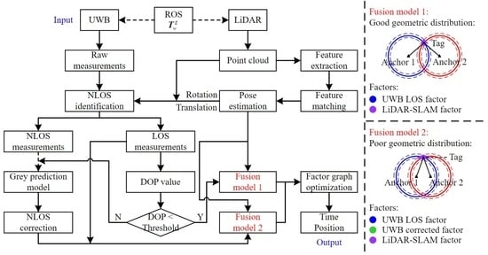
The framework of the proposed FGO-based UWB/LiDAR-SLAM tightly coupled integrated system with NLOS identification and correction using a grey prediction model is shown in
Figure 1. First, the temporal and spatial datums of both the UWB and LiDAR sensors are unified by the robot operating system (ROS) and the calibrated external parameter matrix (purple blocks in
Figure 1). Second, the NLOS identification algorithm using the laser point cloud in our previous work is adopted to distinguish the LOS measurements from NLOS measurements in real-time (green blocks in
Figure 1). Then, the DOP value of the remaining LOS anchors is calculated and compared with a threshold. Suppose this DOP value is higher than the threshold. In that case, the geometric distribution of the remaining LOS anchors is considered poor, the NLOS measurements need to be predicted using the grey prediction model, and the LOS and corrected measurements are used as the inputs to the integrated system (yellow blocks in
Figure 1). Alternatively, only the LOS measurements are used for integrated navigation (blue blocks in
Figure 1), effectively controlling the geometric distribution on the effect of positioning accuracy. Finally, considering that UWB measurements are also affected by signal multipath effects, intensity fading, and other factors, an FGO-based UWB/LiDAR-SLAM integrated system is designed, effectively enhancing the robustness of the integrated system to outliers by using the strong correlation of historical measurements within a sliding window in the time dimension while reducing the possibility of LiDAR-SLAM divergence (orange blocks in
Figure 1). The red dashed block in
Figure 1 represents the contribution of this work.
2.2. Coordinate Frame
A reference datum (coordinate system) is a crucial concept in the study of navigation systems. Sensor measurements, such as position, velocity, and attitude, are based on a description of a reference frame, and the description varies in different frames. The proposed integrated system has two different types of sensors, UWB and LiDAR. It is essential to unify the sensor measurements based on a common coordinate system and establish a functional relationship between the sensor measurements and navigation state information to fuse the measurements of these two types of sensors (as shown in
Figure 2).
w-frame: the UWB coordinate system, with the indoor control point as the origin, x-axis pointing right, y-axis pointing forward, and z-axis forming a right-handed cartesian coordinate system with x-axis and y-axis.
l-frame: the LiDAR coordinate system, moving with the vehicle [
15], with the LiDAR measurement center as the origin,
x-axis pointing forward,
y-axis pointing left, and
z-axis forming a right-handed cartesian coordinate system with
x-axis and
y-axis.
g-frame: the LiDAR-SLAM coordinate system, with the initial LiDAR-SLAM position as the origin, whose axes coincide exactly with the l-frame at the initial LiDAR-SLAM time.
Considering the computational efficiency of the subsequent NLOS identification algorithm using the laser point cloud, the
g-frame is used as the fusion coordinate system in this study. Therefore, the transformation matrix
from the
w-frame to the
g-frame needs to be accurately obtained to unify the measurements. As shown in
Figure 2, the LiDAR sensor can provide precise point cloud data of the surrounding environment in the
g-frame, and the total station can also accurately observe the edges (lines or points) of buildings in the
w-frame. Accordingly, based on the common-view method, this study takes the building edge points as the calibration objects and obtains the UWB anchor coordinates
in the
g-frame and the lever-arm vector
with the laser center pointing to the UWB mobile tag center in the
l-frame by solving the transformation matrix
through the observed multiple corresponding feature point pairs
.
2.3. UWB NLOS Identification Using a Laser Point Cloud Map
As an active sensor, LiDAR can take long-range, high-precision three-dimensional (3-D) measurements of the surrounding environment. LiDAR visually represents objects in the environment in the form of accurate, dense 3-D point clouds while using SLAM 6-DoF pose estimation to register raw laser point clouds into the SLAM coordinate system to obtain a globally consistent map.
Consequently, when positioning is performed in GNSS-denied scenarios, obstacles (fixed interior walls or moving objects) in the NLOS region that are prone to UWB ranging errors are known in the laser point cloud map in terms of their location and size, which is reflected as many point-cloud clusters of varying sizes. Based on this NLOS assumption, the UWB LOS and NLOS measurements can be effectively distinguished by combining the UWB anchor coordinates in the SLAM coordinate system. The NLOS identification algorithm using the laser point cloud consists of three modules: identification preprocessing, point cloud search, and collision detection.
Identification preprocessing module: LiDAR-SLAM is used to deduce the UWB mobile tag coordinate in accordance with the lever-arm vector and the UWB anchor set iterated through to obtain the coordinates of the UWB anchor to be identified for determining the NLOS identification search direction. According to the distance, vertical azimuth, and horizontal azimuth between the mobile tag and anchor, the search center points, and search times are calculated in steps of 1 m.
Point cloud search module: The global map is converted into a k-dimensional tree (KD-tree) structure, and point clouds are searched for in the neighborhood with a radius of 1 m. When the number of point clouds exceeds the set threshold, there may be obstacle occlusion in the line-of-sight direction (i.e., the search direction for NLOS identification); that is, the anchor may be an NLOS anchor.
Collision detection module: To avoid misjudgment and improve the accuracy of NLOS identification, whether the line-of-sight direction intersects with the searched neighboring point cloud cluster is evaluated to distinguish between true and false obstacles and further obtain the LOS anchor set
and NLOS anchor set
. More details of the NLOS identification algorithm using the laser point cloud can be found in [
27].
2.4. Calculation of the HDOP Value for the UWB LOS Anchor
To achieve satisfactory positioning performance of the UWB/LiDAR-SLAM integrated system, in our previous work, the UWB LOS measurements filtered by NLOS identification and the LiDAR-SLAM 6-DoF pose estimation were used as the measurement inputs to the integrated system in a tightly coupled form. Unfortunately, we found that the positioning accuracy of the integrated system is affected not only by the accuracy of the UWB measurements but also by the geometric distribution of the UWB anchors. Using only the LOS measurements can counterproductively introduce a large positioning error to the integrated system when the geometric distribution of the remaining LOS anchors is poor.
Consequently, this study draws on the concept of the DOP value in a GNSS to analyze the goodness of the geometric distribution of the remaining LOS anchors when all NLOS anchors are excluded. The DOP value includes the following parameters: the geometric dilution of precision (GDOP), position dilution of precision (PDOP), horizontal dilution of precision (HDOP), vertical dilution of precision (VDOP), and time dilution of precision (TDOP) [
36]. Since the ground in GNSS-denied environments is mostly flat, this study focuses on the positioning of the integrated system in a two-dimensional (2-D) plane.
Figure 3 shows the effect of different geometric distributions on the 2-D positioning errors. The thicker solid line represents the true ranging value, and the two nearby dashed lines indicate the possible ranging errors. The intersection of the thick solid lines is the true position of the mobile tag. The purple part represents the possible positioning area of the system due to the presence of ranging errors. With the same ranging errors, a smaller HDOP value represents a more uniform geometric distribution of the anchors (
Figure 3a), better positioning performance, and smaller positioning errors. Conversely, a larger HDOP value represents a poorer geometric distribution of the anchors (
Figure 3b), which significantly expands the possible positioning area and increases the positioning error.
The true distance
between the UWB mobile tag
and the
i-th LOS anchor
can be expressed as follows:
Using a Taylor series expansion of the observation equation at the approximate position of the mobile tag
and neglecting components above the second order, we can obtain:
where
where
denotes the directional cosine from an unknown point to a known point in both the
x and
y directions, and
denotes the Jacobian matrix of the distance equation.
The error covariance matrix
and the HDOP value can be obtained as follows:
where
denotes the covariance of the
i-th measurement with the
j-th measurement. The HDOP value is only related to the relative position of the mobile tag and the LOS anchors, independent of the selected coordinates. This positional relationship is the geometric distribution of the UWB system.
2.5. UWB NLOS Correction Using the Grey Prediction Model
If the HDOP value of the remaining LOS anchors fluctuates less and is lower than a threshold, subsequently, when fusing the data with LiDAR-SLAM, all NLOS measurements can be excluded, and only the filtered LOS measurements will be used as the measurement input. Otherwise, considering that the NLOS anchors have a great effect on the geometric distribution of the UWB anchors, excluding the NLOS anchors will lead to a poorer geometric distribution, which will impact the positioning accuracy.
This study proposes an NLOS correction method using a grey prediction model to improve the reliability of the positioning system [
37]. When the HDOP value of the remaining LOS anchors is higher than a threshold, all existing NLOS measurements are discarded, and the NLOS measurements are instead predicted using a grey prediction model based on a small number of historical measurements to obtain the corrected measurements, which are used together with the LOS measurements as the inputs to the integrated system. The inclusion of the corrected measurements better improves the geometric configuration of the original LOS anchors and minimizes the HDOP value of the positioning system, thereby effectively improving the positioning accuracy and robustness of the system. The NLOS correction method process using the grey prediction model is as follows.
where
denotes the nonnegative original time series; the subscripts
n and
m denote the number of UWB anchors and measurements, respectively;
denotes the
u-th historical measurement of the
i-th UWB anchor; and this study uses
.
- 2.
A first-order accumulated generation operation on the original data is performed to obtain a new data sequence with an approximate exponential law, aiming to reduce the impact of randomness and volatility on the data:
where
.
- 3.
The consecutive neighborhood sequence C(1) of sequence R(1) is as follows:
where
, and
.
- 4.
The grey differential equation of the GM(1,1) model is established according to the approximate exponential law:
where
denotes the background value of the grey differential equation and
and
denote the development coefficient and the grey action quantity, respectively, which can be solved for using the least squares (LS) method:
where
where
Y denotes the historical measurement vector, and
B denotes the sequence matrix.
- 5.
The whitening function for the differential equation is constructed using the solution to the above equation:
Thereby, the time response sequence of the grey differential equation is obtained as:
- 6.
Finally, the inverse transformation operation of Equation (12) is performed to obtain the prediction function of the original sequence of the i-th UWB anchor as follows:
The GM(1,1) model established by the UWB historical measurements (epoch 1 to epoch m) can be used to predict the NLOS measurement (epoch m + 1) when the HDOP value of the remaining LOS anchors is higher than the threshold. Meanwhile, after obtaining the corrected measurement (epoch m + 1), the initial measurement of the original sequence is discarded, and the remaining measurements (epoch 2 to epoch m) and the new measurement (epoch m + 1) are formed into a new sequence. The relevant parameters of the grey prediction model are recalculated to better accommodate the volatility of the measurements.
2.6. UWB/LiDAR-SLAM Integrated Model Based on Factor Graph Optimization
Filtering [
38,
39,
40] and graph optimization [
41,
42,
43] are the two main schemes for multisensor data fusion. A Bayesian filtering-based method finds the best estimate of the current state through prediction-measurement-correction, which has the advantages of low computational complexity and high accuracy. As an information transfer model, the optimization methods represented by factor graphs model the observed data as a kind of factor graph network with data association. Unlike the former, which only considers the state information of the last epoch and the measurements of the current epoch, the factor graph performs nonlinear optimization of the overall or partial state data set based on all or part of the historical measurements and the current measurements. Due to the temporal correlation between measurements and the redundant measurements of the system, the integrated system tends to achieve more accurate and robust state estimations.
The framework of the FGO-based UWB/LiDAR-SLAM integrated system is shown in
Figure 4, where both the UWB LOS and corrected measurements are tightly coupled to LiDAR-SLAM without loop closure using FGO. The navigation system states are represented by the variable nodes (hollow circles), and the a priori information, state transitions, and measurement processes are represented by the factor nodes (solid circles). As seen, the graphical representation makes the system highly versatile and extensible, allowing for the flexible combination of sensor information with different measurement frequencies and effectively coping with sensor failure or the introduction of new sensor information.
The goal of multisensor data fusion is to find the optimal posterior state of the system given the sensor measurements, which is a typical maximum a posteriori (MAP) estimation problem [
41,
44]. In this study, the measurements include UWB and LiDAR-SLAM measurements. Assuming that the UWB and LiDAR-SLAM measurements are independent of each other, the state estimation problem of the UWB/LiDAR-SLAM integrated system can be formulated as the following MAP problem:
where
denotes the set of system states to be estimated;
denotes the state vector;
and
denote the 3-D translation and rotation (denoted by a quaternion) between the
l-frame and
g-frame, respectively;
denotes the set of system optimal states;
z denotes the sensor measurements associated with state
x.
For any factor graph, the MAP problem can be reduced to maximizing the product of all factor graph potentials [
45]:
where
denotes the factor associated with the measurements.
In an FGO-based integrated model, the sensor measurements are all considered as factors
associated with the particular state
x, each of which represents an error function that should be minimized. Supposing that all sensor measurements are disturbed by Gaussian noise with a zero mean, the negative logarithm of
is proportional to the error function associated with the measurement and is defined as follows:
where
and
z denote the observation functions and actual measurements of different positioning systems, respectively; the Mahalanobis norm is
, which takes into account the effect of the observation accuracy;
denotes the covariance matrix of the observation process, in which the UWB and LiDAR-SLAM uncertainties are determined based on the ranging accuracy and the degree of matching, respectively; and
denotes the Euclidean norm of the vector.
Taking the negative logarithm of Equation (15) and discarding the coefficient terms, the MAP problem can be transformed into a nonlinear least squares (NLS) problem:
where the superscripts
and
denote the number of UWB measurement residuals and LiDAR-SLAM measurement residuals; the superscript
n denotes the number of UWB anchors; the subscripts
j and
k denote the indexes of UWB factors and LiDAR-SLAM factors in the factor graph; the subscript
i denotes the index of UWB anchors;
denotes the UWB anchor coordinates;
denotes the measurement residuals associated with the UWB sensor (residuals of ranging); and
and
denote the measurement residuals associated with the LiDAR sensor (residuals of translation and rotation). The error functions with UWB and LiDAR-SLAM factors are as follows:
where
denotes the multiplication operator of the quaternion;
denotes the actual UWB measurements; and
and
denote the actual LiDAR-SLAM measurements.
By minimizing the above objective function, the maximum a posteriori solution
of the state set can be obtained, and thus, multisensor data fusion can be realized. Considering that the computation amount will increase significantly with the increase in the factor graph scale as new measurement information is continuously added over time, this study adopts a sliding window method [
46] to maintain the relative stability of the number of optimized variables by discarding the earliest historical variables in the window while adding new variables.
3. System Performance Testing and Analysis
3.1. Platform Description and Experimental Setup
We build an integrated positioning experimental platform to test the proposed NLOS correction method using the grey prediction model and the FGO-based UWB/LiDAR-SLAM integrated system. All algorithms are implemented and evaluated on a computer with an Intel(R) Core(TM) 2.30 GHz i7-10875H central processing unit (CPU), 32 GB of RAM, and an Nvidia GeForce RTX 2060 graphics card, running a 64-bit Linux (Ubuntu 18.04) operating system. As shown in
Figure 5, a Velodyne VLP-16 scanner is installed in the center of the experimental platform, and a Time Domain UWB PulsON440 module and 360° total reflection prism are installed above the laser scanner. The centers of all three are on the same plumb line; therefore, the effect of the lever-arm on the integrated navigation in the 2-D plane can be ignored. The specifications of the UWB and LiDAR sensors are shown in
Table 1. Considering the high-precision performance of the Leica TS50 automatic tracking total station, it is assumed that its measured UWB anchor 3-D coordinates and the starting coordinates of the UWB mobile tag and LiDAR sensor when the experimental platform is stationary are error-free. In the dynamic test, the total station automatically tracks the total reflection prism and provides the reference with an accuracy of
every 0.1 s.
A dynamic experiment is conducted in an underground parking lot of a shopping mall, and the experimental scenario and layout are shown in
Figure 6. We deploy six UWB anchors in a 40 m × 40 m area to better demonstrate the UWB positioning accuracy fluctuation under a poor geometric distribution. The presence of many moving objects (passing pedestrians and vehicles) and stationary objects (wall pillars (70 cm × 70 cm) and stationary vehicles) in the underground parking lot makes the environment very challenging. For the total station to effectively track the experimental platform and provide an accurate reference trajectory, an evaluation dataset is obtained using ROS by an experimenter pushing the experimental vehicle along a travel lane (purple route) at a speed of 0.5 m/s. The parking space areas are not planned into the travel route considering the continuity of the reference trajectory.
3.2. Evaluation of the UWB NLOS Identification and Correction Algorithm
To evaluate the effectiveness of the proposed NLOS correction method using the grey prediction model, the time-synchronized UWB raw, LOS, and corrected measurements are all variously used as the inputs to the LS positioning method, and the following three methods are obtained for comparison:
LS positioning using the raw measurements (LS);
LS positioning using the LOS measurements (NLOS identification + LS, NI-LS);
LS positioning using the LOS and corrected measurements (NLOS identification + NLOS correction + LS, NINC-LS).
Figure 7 shows a comparison of the three UWB measurements with the reference measurement. The error curves between the measurements after discarding the zero value and the reference value are shown in
Figure 8 (the subgraphs above the figures are enlarged details of the error curves).
Table 2 reports the statistical results of the ranging errors for the three measurements. ‘RMSE’ in the table stands for the root mean square error, and ‘Max’ stands for the maximum error.
Figure 9 shows the UWB positioning trajectories solved using the LS, NI-LS, and NINC-LS methods.
Figure 10 shows the positioning errors of these three methods in the X, Y, and plane directions and the cumulative distribution function (CDF) of the plane errors. The specific evaluations are shown in
Table 3. ‘Availability’ in the table is calculated by dividing the number of solved positions by the total number of measurements.
It can be observed that the experimental scenario of the underground parking lot is challenging for the UWB positioning system. During the travel process, there are many measurement outliers in the UWB raw measurements due to obstacle occlusion. Anchors 1, 2, and 6 have lower ranging accuracy due to their poor surrounding environments (all are located near wall columns), with RMSEs of 0.8178 m, 1.3146 m, and 1.2918 m, respectively. Anchor 2 astonishingly has a maximum ranging error of 36.5315 m. Although the placements of anchors 3, 4, and 5 are more ideal, the RMSEs also reach 0.5012 m, 0.4089 m, and 0.4225 m, which are far below the accuracy level under the UWB line-of-sight. After filtering using the NLOS identification algorithm, the data quality of LOS measurements is significantly improved. Compared with the raw measurements, the ranging accuracy of UWB anchors is improved by 92.88%, 95.98%, 88.47%, 79.24%, 78.34%, and 93.84%. Correspondingly, the NI-LS method using LOS measurements has been considerably improved. Compared with the LS method, the RMSEs of the positioning errors in the X, Y and plane directions are reduced by 85.04%, 76.28%, and 79.60%, respectively, and the maximum errors are reduced by 92.80%, 92.05%, and 92.24%, respectively.
Nevertheless, we find that the solved trajectory of NI-LS still partially deviates from the reference trajectory, as shown in the purple dashed region in
Figure 9. Taking the cyan point as an example, when the experimental platform moves to the current position, it receives the measurement from anchors 1, 2, 3, 5, and 6, of which anchor 2 is identified as an NLOS anchor. Interestingly, although the ranging accuracy of the remaining LOS anchors generally reaches the subdecimeter level (0.138 m, 0.110 m, 0.136 m, and 0.020 m), the plane error of its solved position still reaches 0.487 m. This result indicates that using only the filtered LOS measurements as the input to the positioning system may still fail to meet the needs for indoor high-precision positioning. This is because the excessive rejection worsens the geometric distribution of the system, and the complete exclusion of the NLOS measurements reduces the system’s availability by 2.81%.
Figure 11 shows a comparison between the HDOP value and the NI-LS method error. After effective data quality control, the positioning error of the system is approximately positively correlated with the HDOP value, and variances within different intervals (e.g., 0–50 s) are caused by different levels of ranging accuracy. Therefore, to ensure the robustness of the system, considering the geometric distribution of the remaining LOS anchors during the positioning solution is essential.
The corrected ranging values obtained using the proposed method are shown in
Figure 9. Based on the threshold judgment principle, the method corrects some of the NLOS measurements to obtain the corrected measurements.
Table 2 shows that the corrected measurements maintain almost the same ranging accuracy as the LOS measurements, and the NINC-LS method using the LOS and corrected measurements subsequently achieves a corresponding improvement. In the purple dashed region where the NI-LS solution is worse, the NINC-LS method significantly improves the overall performance of the system under the poor geometric distribution, making it more closely fit the reference trajectory. Compared with the LS and NI-LS methods, the RMSEs of the positioning errors in the X, Y, and plane directions are reduced by 87.56%, 85.30%, and 86.26% and 16.84%, 38.01%, and 32.65% for the NINC-LS method, respectively. The RMSE in the plane direction is reduced to 0.132 m, which provides solid evidence for the rationality and effectiveness of the proposed method. However, the maximum error improvement is not obvious.
Figure 12 shows the number of NLOS measurements for the NI-LS and NINC-LS methods. After correction using the proposed method, the number of NLOS measurements is less than or equal to 3. While outputting high-precision positioning results, the system’s availability reaches 100%, even better than the raw measurement value (99.65%).
3.3. Evaluation of the UWB/LiDAR-SLAM Integrated Positioning Algorithm
The solved trajectories are compared with those of the single sensor, and five other UWB/LiDAR-SLAM integrated positioning methods to test the effectiveness of the proposed FGO-based UWB/LiDAR-SLAM tightly coupled integrated system with NLOS identification and correction using the grey prediction model (NLOS identification + NLOS correction + tightly coupled + FGO, NINC-FGO).
NINC-LS;
LeGO-LOAM without loop closure;
Tightly coupled + REKF (REKF);
NLOS identification + tightly coupled + REKF (NI-REKF) [
27];
NLOS identification + NLOS correction + tightly coupled + REKF (NINC-REKF);
Tightly coupled + FGO (FGO);
NLOS identification + tightly coupled + FGO (NI-FGO).
Figure 13 shows a comparison of the trajectories estimated using the different methods with the reference trajectory. The positioning errors of these eight methods in the X, Y, and plane directions and the CDF of the plane errors are shown in
Figure 14.
Table 4 reports the positioning performance of each method. In the table, the red, blue, and green results represent the best, second-best, and third-best accuracies, respectively.
As seen in
Table 4, the REKF method significantly improves the positioning performance of the integrated system by adjusting the measurement noise covariance matrix to reduce the contribution of abnormal measurements to parameter estimation when the UWB raw measurements polluted from NLOS errors are used directly as the input to the integrated system. It outperforms the NI-LS method (RMSEs in the X, Y, and plane directions are reduced by −2.53%, 19.81%, and 11.36%, respectively) and LeGO-LOAM (RMSEs in the X, Y, and plane directions are reduced by 16.49%, 6.59%, and 12.03%, respectively). However, the FGO method, which assigns the same weights to measurements of different qualities, achieves a positioning accuracy inferior to that of a single sensor (NINC-LS or LeGO-LOAM methods). Furthermore, if we define the availability as the error below 0.1 m due to the temporal correlation between measurements and the redundant system measurements, the FGO method (74.95%) is far superior to the REKF method (57.36%).
The advantages of the integrated positioning methods are manifested when the raw measurements are filtered once using the NLOS identification method. Both the NI-REKF and the NI-FGO methods achieve better accuracy than that of a single sensor. Compared with the conventional integrated model (REKF or FGO methods), the RMSEs of the positioning errors in the X, Y, and plane directions are reduced by 1.23%, 14.12%, and 7.69% and 38.74%, 37.62%, and 38.67%, respectively. Meanwhile, the NI-FGO method outperforms the NI-REKF method, reducing the RMSEs of the positioning errors in the X, Y, and plane directions by 15.00%, 13.70%, and 14.81%, respectively.
Comparing the six UWB/LiDAR-SLAM integrated positioning methods, whether the REKF-based integrated framework or the FGO-based integrated framework, the proposed methods (NINC-REKF and NINC-FGO methods), which use the LOS and corrected measurements as the inputs to the integrated system, achieve optimal results in their respective frameworks. Such improvements illustrate that the proposed methods for controlling the sensor data quality (NLOS identification + NLOS correction) can effectively improve the positioning performance of the UWB/LiDAR-SLAM integrated system. Compared with the REKF and NI-REKF methods, the RMSEs of the NINC-REKF method in the X, Y, and plane directions are reduced to 0.071 m, 0.069 m, and 0.099 m, respectively. Compared with the FGO and NI-FGO methods, the RMSEs of the NINC-FGO method in the X, Y, and plane directions are reduced to 0.062 m, 0.060 m, and 0.086 m, respectively. Similarly, the NINC-FGO method achieves better results than the NINC-REKF method (RMSEs in the X, Y, and plane directions are reduced by 12.68%, 13.04%, and 13.13%, respectively), and even the NI-FGO method outperforms the NINC-REKF method (RMSEs in the X, Y, and plane directions are reduced by 4.23%, 8.70%, and 7.07%, respectively), which fully demonstrates the superiority of the FGO-based UWB/LiDAR-SLAM integrated model.
Since the system models are designed based on a tightly coupled model, the availability of the six integrated methods is 100%. Similarly, if we define the availability as the error below 0.1 m, then it can be seen from
Figure 14d that the FGO-based integrated models all outperform the REKF-based integrated models. The availability of the NINC-FGO method is as high as 77.93%, which is better than that of any other method. In summary, the NINC-FGO method performs best when both accuracy and availability are considered, which fully verifies the superiority and accuracy of the proposed UWB/LiDAR-SLAM integrated system.
4. Conclusions
A UWB/LiDAR-SLAM integrated system is an effective solution to address the difficulty of precise positioning in GNSS-denied environments. However, the existence of UWB NLOS errors will affect the accuracy and effectiveness of the integrated system to varying degrees. For better fusion, we do the following. First, we use our previous work on UWB NLOS identification and exclusion to strictly control the data quality of the system input. Second, considering that the system positioning accuracy is affected not only by the ranging accuracy but also by the geometric distribution of UWB anchors, we calculate the HDOP value of the remaining LOS anchors to evaluate the layout accuracy. Then, for a poor geometric distribution, we propose an NLOS correction method using a grey prediction model. The high accuracy and robustness of the integrated system are effectively maintained by increasing the measurements. Finally, an FGO-based UWB/LiDAR-SLAM tightly coupled integrated system is designed. The evaluations of the dynamic positioning experiment show the following. (1) The corrected measurements constructed using the grey prediction model maintain almost the same ranging accuracy as the LOS measurements. The NINC-LS method using the LOS and corrected measurements as the system inputs also achieves satisfactory results, with the RMSE in the plane direction reduced to 0.132 m and the availability of errors below 0.1 m reaching 60.31%, proving the effectiveness of the proposed NLOS correction method. (2) The proposed FGO-based integrated models are all superior to the REKF-based integrated models. The NINC-FGO method takes the optimal positioning effect and robustness, with an RMSE of 0.086 m in the plane direction and 77.93% availability of errors below 0.1 m, thus fully demonstrating the superiority of the proposed method. In the future, our work will include the integration of the existing integrated system with low-cost inertial measurement units (IMUs) to enhance the accuracy and robustness of the positioning system in highly dynamic and degrading environments.


