


Fast Distributed Multiple-Model Nonlinearity Estimation for Tracking the Non-Cooperative Highly Maneuvering Target
College of Aerospace Science and Engineering, National University of Defense Technology, Changsha 410073, China
*
Author to whom correspondence should be addressed.
Remote Sens. 2022, 14(17), 4239; https://doi.org/10.3390/rs14174239
Submission received: 20 July 2022
/
Revised: 20 August 2022
/
Accepted: 25 August 2022
/
Published: 28 August 2022
(This article belongs to the Special Issue Distributed Spaceborne SAR: Systems, Algorithms, and Applications)
Abstract
:The newly developed near-space vehicle has the characteristics of high speed and strong maneuverability, being able to perform vertical skips and a wide range of lateral maneuvers. Tracking this kind of target with ground-based radars is difficult because of the limited detection range caused by the curvature of the Earth. Compared with ground-based radars, satellite tracking platforms equipped with Synthetic Aperture Radars (SARs) have a wide detection range, and can keep the targets in custody, making them a promising approach to tracking near-space vehicles continuously. However, this approach may not work well, due to the unknown maneuvers of the non-cooperative target, and the limited computing power of the satellites. To enhance tracking stability and accuracy, and to lower the computational burden, we have proposed a Fast Distributed Multiple-Model (FDMM) nonlinearity estimation algorithm for satellites, which adopts a novel distributed multiple-model fusion framework. This approach first requires each satellite to perform local filtering based on its own single model, and the corresponding fusion factor derived by the Wasserstein distance is solved for each local estimate; then, after diffusing the local estimates, each satellite performs multiple-model fusion on the received estimates, based on the minimum weighted Kullback–Leibler divergence; finally, each satellite updates its state estimation according to the consensus protocol. Two simulation experiments revealed that the proposed FDMM algorithm outperformed the other four tracking algorithms: the consensus-based distributed multiple-model UKF; the improved consensus-based distributed multiple-model STUKF; the consensus-based strong-tracking adaptive CKF; and the interactive multiple-model adaptive UKF; the FDMM algorithm had high tracking precision and low computational complexity, showing its effectiveness for satellites tracking the near-space target.
1. Introduction
Target tracking has been extensively researched and widely used in areas such as situational awareness, precision navigation, and marine surveillance [1,2]. However, accurate non-cooperative target tracking remains challenging, due to the unknown maneuvers of the targets. Recently, newly developed high-speed near-space vehicles have been widely investigated [3,4,5]. Non-cooperative near-space vehicles can perform diverse maneuvering modes, including vertical skips and a wide range of lateral maneuvers, posing higher requirements for tracking technology.
Generally, observation platforms can be separated into two main categories in target tracking: ground-based radar [3,6] and satellites [7]. Although ground-based radars are widely used in target tracking, they cannot guarantee the near-space target to be in custody, due to the limited detection range caused by the curvature of the Earth. In contrast, satellites have the advantage of a wide detection range, and thus they are feasible for tracking near-space targets. Spaceborne Synthetic Aperture Radar (SAR) systems have large imaging coverage, and can provide high-quality measurements, which are suitable as detection devices for satellite tracking systems [8,9,10]. The techniques of satellite tracking systems whose objects are mainly space orbital targets have been researched in recent years [11,12,13], while few studies have been conducted for near-space targets. Unlike the tracking of space orbital targets, there are two main issues in tracking near-space targets: (1) the maneuvers of the target are unknown and diverse, and thus a high-precision and stable tracking algorithm is required; (2) the computing power of satellites is limited; hence, an algorithm with low computational complexity is demanded. It has been necessary, therefore, to develop a tracking algorithm with high tracking accuracy, strong stability, and high computational efficiency for satellites tracking non-cooperative near-space targets.
The frameworks of multiple satellites tracking algorithms can generally be divided into ‘centralized’ and ‘distributed’. In centralized tracking algorithms [14,15], a central satellite is required to communicate with the remaining satellites, i.e., to receive and process data from them. Centralized tracking algorithms therefore usually impose a substantial computational burden on the central satellite. Moreover, the centralized framework relies heavily on the central satellite, meaning that the tracking system will break down once the central satellite fails. In contrast, in the distributed framework, no central node is needed [16], and the computing tasks of the entire network can be allocated to each satellite, which significantly speeds up the computing efficiency of the tracking system. Each satellite only exchanges data with adjacent satellites [15]. Even if one satellite fails, the tracking system, as a whole, will not break down. Due to this high computing efficiency and high resistance to satellite faults, the distributed framework is therefore more appealing.
To improve tracking precision, numerous motion models have been developed in recent years, to more accurately describe the state transition of the target, such as the Constant Velocity (CV) model, the Constant Acceleration (CA) model, and the Singer model [17]. However, a single model may not work well when the target maneuvers. Various Multiple-Model (MM) methods have been proposed, to resist maneuvering uncertainty by using combinations of multiple models [1,2,18,19]. Unlike the mechanism in MM methods, where each elemental filter works individually, an Interactive Multiple Model (IMM) can adaptively track maneuvering targets via the efficient interaction of each filter, which assigns weights to each sub-model according to the model likelihood and mode probability at each moment [20,21,22]. MM methods are usually designed for centralized frameworks, and cannot be directly applied to distributed tracking.
In distributed tracking algorithms, consensus-based algorithms are widely used [15,16,23,24,25,26,27,28,29]. This enables state estimations or measurements from each node to attain the same value, through a consensus protocol, and guarantees global convergence [16]. To deal with the target maneuver, a Consensus-based Distributed Multiple Model UKF (CDMM-UKF) algorithm has been proposed, based on the IMM in [23]. However, when the model set mismatches the target motion, the competition between sub-models cannot be ignored. In addition, each satellite needs to run multiple filters in every filtering period, and to exchange data frequently to reach a consensus, which also creates a considerable communication and computational burden. The Strong Tracking Filter (STF) is suitable for dealing with model mismatches [6,24,30,31,32,33]. The STF can reduce the impact caused by the motion model error, by enlarging the predicted state covariance based on the innovation sequence orthogonal principle [30]. To eliminate the effect of the dynamics model error, a Consensus-based Strong Tracking Adaptive Cubature Kalman Filtering (CSTACKF) algorithm has been proposed in [24]. This distributed algorithm combines the advantages of consensus and adaptive filter, to resist maneuver uncertainty. However, as the CSTACKF algorithm adopts a single motion model, the tracking stability of the CSTACKF algorithm cannot be guaranteed when tracking non-cooperative targets with intense maneuvers.
To improve the stability and precision of satellite tracking systems, the aim of this paper was to develop a new distributed algorithm based on the MM approach and STF. To further cope with the computational burden brought about by the MM, a novel distributed MM framework was put forward for the algorithm, to reduce the computation complexity for each satellite. The proposed algorithm was termed the Fast Distributed Multiple-Model (FDMM) algorithm. The main idea of the FDMM algorithm is as follows: firstly, each satellite performs a local estimation, based on its single motion model and an adaptive CKF algorithm; then, the corresponding fusion factor derived by the Wasserstein distance is solved for each local estimate; secondly, after diffusing the local estimations, each satellite performs multiple-model fusion on the received estimations, based on the minimum weighted Kullback–Leibler (KL) divergence. Finally, each satellite updates its state estimation according to the consensus protocol. The contributions of this study are summarized as follows:
- (1)
- A novel distributed multiple-model fusion framework was proposed, to lower the computational burden for the satellites. Unlike the mechanism in a distributed MM [23,25], where each satellite needs to process multiple filters in the local estimation process, each satellite in the FDMM algorithm only needs to process one filter, based on one motion model in the local filtering process.
- (2)
- The Wasserstein distance with triangular inequality and symmetry is applied, to derive weight factors for each sub-model, to deal with the sub-model competition problem in MM.
The remainder of this paper is organized as follows: Section 2 presents the related works on the fading factor and topology; Section 3 gives the problem formulation; in Section 4, the proposed FDMM tracking algorithm is introduced in detail; the effectiveness and advantages of the FDMM algorithm are demonstrated in two simulation experiments in Section 5; finally, Section 6 concludes our study.
2. Related Works
2.1. Fading Factor
The STF is appealing, for tracking non-cooperative maneuvering targets. The core part of the STF is the fading factor, , which can reduce the impact caused by the motion model error. When a dynamics model mismatch occurs, the value of the fading factor, , is enlarged, and the prediction covariance matrix, , is also enlarged by , in real time. This process reduces the contribution of the dynamics model, and improves the adaptability of the tracking algorithm to motion-modeling uncertainty [30].
Based on the mutual orthogonality between innovation sequences, the fading factor, , can be expressed as Equation (1):
where denotes the covariance of the innovation vector, quantifying the dynamics error; this is usually estimated according to Equation (2):
where is the innovation, and is the forgetting factor, determined to be .
2.2. Topology
The communication topology of the satellites at time can be represented by a graph, , where vertexes are the set of all satellites, and edges present the communication connection between the satellites. The set of adjacent satellites of the satellite is expressed as .
At time , the communication protocol between satellite and its adjacent satellite, , is set as the Metropolis matrix, [12], as shown in Equation (3):
where are indices of satellites.
3. Problem Formulation
3.1. Tracking Formulation
The dynamics and observation functions of the maneuvering target-tracking process are modeled as follows:
where and are the state vector and measurement vector of the maneuvering target at time , respectively; is the state transition function; is the process noise; and and are the measurement function and the measurement noise, respectively.
3.2. Measurement Model
Satellites operating in low orbits are applied to detect the target. As shown in Figure 1, a single satellite can provide two measurements of the target through processing SAR images, consisting of the azimuth, , and the elevation angle, . The detecting coordinate system is paralleled to the Earth-Centered Inertial (ECI) [34].
For satellite , the measurement model at time is described as Equation (6):
where the position of satellite, , and the target in ECI are and , respectively; and are noises in the corresponding measurement channels.
If , , Equation (6) can be further compacted into a measurement model of the standard form in Equation (7):
where is the measurement function of satellite . The measurement noise, , is modeled with the zero-mean Gaussian noise . The schematic diagram of multiple satellites tracking the target is shown in Figure 2.
4. Fast Distributed Multiple-Model Nonlinearity Estimation Algorithm
The traditional distributed multiple-model algorithms in [23,25] cannot track a non-cooperative highly maneuvering target stably, and impose a substantial computational burden on each satellite. Therefore, to reduce the computational burden and improve the tracking accuracy of the satellites, the Fast Distributed Multiple-Model (FDMM) nonlinearity estimation algorithm, combined with the adaptive Cubature Kalman filter, is put forward in this section.
In the FDMM algorithm, a novel distributed multi-model fusion framework is adopted to assign the computational tasks of MM filtering to each satellite. Unlike the framework in [23,25], where each node performs multiple filtering based on multiple-motion models, the FDMM algorithm allows each satellite to perform local filtering based only on a single but different motion model. After local filtering, the local estimates of each satellite are diffused to adjacent satellites, and then multiple-model fusion is performed on the obtained results in each satellite.
To deal with the motion model mismatches engendered by the non-cooperative target, the adaptive CKF algorithm, based on the fading factor for local filtering, is first introduced below. Next, the newly proposed fusion factor and the multiple-model fusion framework based on weighted KL divergence are introduced, to fuse each satellite’s obtained local estimation results.
4.1. Strong-Tracking Cubature Kalman Filter
Based on the fading factor, , shown in Equation (1), the strong-tracking CKF can be achieved by the following steps:
- Compute the cubature points at time :where is the Cholesky factor of ; denotes the dimension of the state ; and represents weighted coefficients of the ; the being the -th column of the following matrix:
- Time update:where, refers to the corresponding innovation sequence.
- Fading factor update:
- Measurement update:
4.2. Fusion Factor Derived from the Wasserstein Distance
As the detailed motion characteristics of the non-cooperative target cannot be obtained, a single model cannot work well when the target maneuvers. Considering that conventional distributed MM methods engender a substantial computational burden, we have proposed a new distributed multiple-model mechanism to cope with the target maneuvers, and to reduce the computational burden. Each satellite first performs local filtering based on a single but different motion model, then performs multiple-model fusion on the data obtained from adjacent satellites. By allocating the computing tasks of the MM filtering process to each satellite, the computational efficiency of the tracking system is significantly improved.
The distance function and fusion factor are introduced in this section. They are the core parameters for performing the fusion of distributed multiple-model estimations in the FDMM algorithm.
4.2.1. Distance Function
Before performing multiple-model fusion, it is necessary to evaluate the similarity of the current model to the actual motion mode of the target. In the traditional multiple-model algorithm, the model likelihood function, , represents the Gaussian probability of classifying the current mode of the target to the i-th model based on the measurement , and is solved as shown in Equation (29):
where is the innovation, and is the variance of the innovation.
In the proposed distributed algorithm, the measurements used by each satellite are different. Each satellite has different measurement errors. It is not appropriate to still use the model likelihood function, based on the respective measurements, to calculate the Gaussian probability of the model. Therefore, we introduced the Wasserstein distance [35,36], to evaluate the distance between the using model and the current motion mode.
Definition 1.
When , the Wasserstein distance has the following properties: symmetry and triangle inequality [35,36]. The properties of Wasserstein distance make it a good metric for evaluating the similarity between the used model and the target mode.
Specifically, for two Gaussian distributions, we can solve for their Wasserstein distance by Equation (31):
The measurement that satellite obtains at time can be expressed as Equation (32):
where represents the ideal measurement that does not contain noise.
The predicted measurement, , can be obtained according to Equation (18) at the satellite , and follows a Gaussian distribution, i.e., . Therefore, the similarity between the using model and the current motion mode can be quantified by the Wasserstein distance between the predicted measurement, , of local filtering, and the ideal measurement, , where .
According to Equation (31), we can compute the Wasserstein distance, , between the using model and the current motion mode as Equation (33):
4.2.2. Fusion Factor
After local filtering, the local estimates of each satellite are diffused to adjacent satellites. Before performing multiple-model fusion on the data, it is necessary to assign weights to the data from each satellite. The Wasserstein distance, , based on Equation (33), describes the distance between the model and the target motion mode. The smaller is, the closer the i-th model is to the target mode. In this paper, according to the characteristics of , the fusion factor was introduced, to evaluate the similarity of each local estimate in the FDMM algorithm.
Definition 2.
Assuming that the Wasserstein distance between the i-th motion model and the current motion mode at time k is , the fusion factor, , in the FDMM algorithm is defined as Equation (34).
The local estimates and the fusion factor of each satellite are simultaneously diffused to their adjacent satellites. According to the corresponding fusion factor, , the weight of each estimation obtained at the satellite can be calculated by Equation (22):
where refers to the weight of the estimation from the adjacent satellite, at the satellite , so .
4.3. Multiple-Model Fusion Based on Weighted KL Divergence
After each satellite receives the local estimates and the corresponding fusion factor, the multiple-model fusion is performed. This section takes the satellite as an example, to introduce how each satellite performs multiple-model fusion on the received data. Firstly, the satellite obtains the local estimation and corresponding fusion factor from the adjacent satellites. Secondly, based on the weighted sum minimization of the information entropy, a probability density function (PDF) is found, as the multiple-model fusion results that minimize the difference between the PDFs of the received estimations.
In order to solve the problem of multiple-state estimation fusion, combined with reference [37,38], the definition of weighted KL divergence is introduced.
Definition 3.
Given N PDFs, and relative weightssatisfying Equation (36),
their weighted KL average (KLA) is defined by Equation (37):
Lemma 1.
The weighted KLA defined in Equation (37) is given by Equation (38):
Lemma 2.
If all the PDFstake the Gaussian PDF form, their weightssatisfying Equation (36), their weighted KLA in Equation (38) takes the form of Equation (39):
then the meanand the covariancecan be computed from Equations (40) and (41):
The proof of Lemmas 1 and 2 can be found in [37].
After filtering, each satellite can obtain the local state estimation —where —the covariance , and the corresponding fusion factor, , through communication. Then, we can obtain the weight of each estimate, according to Equation (35). Because each local estimate is a Gaussian distribution, with mean and variance , we can approximate all obtained local estimates, , using a Gaussian distribution at satellite , based on lemma 1 and lemma 2. Then, we can get the multiple-model fusion results, , , from Equations (42) and (43), based on Weighted KL Divergence:
4.4. Fusion Framework
In the FDMM algorithm, a novel distributed multiple-model fusion framework is proposed, to reduce the computational burden of the tracking system by allocating tasks to each satellite. The fusion framework is introduced below. Each satellite performs local estimations, based on its own single-motion model. The motion model selecting rules that determine which satellite adopts which motion model are also discussed in this section.
4.4.1. Fusion Framework
The operation flow of satellite , from time to time , adopting the FDMM algorithm, is shown in Figure 3. Firstly, each satellite runs a different single-motion model, combined with the STCKF algorithm—based on the augmentation measurements from the adjacent satellites—and calculates the fusion factor, , derived from the Wasserstein distance. Then, the local estimates, , , and are exchanged with the adjacent satellites via the topology net. Then, multiple-model fusion is performed, based on the weighted KL divergence for the received state estimates from different motion models. Finally, each satellite updates its state estimation according to the consensus protocol.
4.4.2. Motion Model Selecting Rules
When deciding which motion model to choose for which satellite, the following two aspects are mainly considered. Firstly, construct a suitable model set, which contains the motion models that will be used. The set needs to describe the maneuvers of the target as much as possible. The CV model describes targets without maneuverability, and the CA is modeled for targets with constant acceleration in each sampling interval. The Singer models with different parameters (the maneuvering frequency, , and the acceleration variance, ) could represent the targets with different maneuvering capabilities [17]. Considering the characteristics of the models, the CA model, the CV model, and the Singer model were chosen as the element of the model set in this paper, to deal with the maneuvers of the non-cooperative target.
Secondly, the topology of satellites is a significant constraint to be aware of, when assigning the motion model to the satellite. In the FDMM algorithm, after the local filtering, each satellite performs multiple-model fusion on the received estimations solved by adjacent satellites. Therefore, the motion models used by adjacent satellites can affect this satellite’s multiple-model fusion results. If the neighbors of one satellite, and that satellite itself, all adopt the CV model, the multiple-model fusion results for that satellite will be at their worst when the target maneuvers. In addition, if the neighbors of one satellite, and that satellite itself, all adopt the CA model, the multiple-model fusion results of that satellite will also be poor when the target starts moving at a constant speed. Therefore, when assigning the motion model to each satellite, it is necessary to ensure that at least two models exist in each satellite and in its neighbors. One model is used to model the weak maneuvering or non-maneuvering situation of the target—such as the CV or the Singer with —and the other is used to model the situation where the target performs maneuvers, such as the Singer with or CA. Furthermore, after the multiple model fusion process, each satellite will update its state estimation according to the consensus protocol. In the consensus update process, each satellite can affect the outcome of the tracking system. Therefore, the satellite tracking system should use the motion models from the model set, as much as possible.
4.5. Implementation Steps of FDMM Algorithm
The FDMM algorithm applying to the satellite , from time to time , is shown in Algorithm 1.
| Algorithm 1 Fast Distributed Multiple-Model (FDMM) Nonlinearity Estimation |
|
|
|
5. Simulation and Discussion
In this paper, we focused on tracking a non-cooperative target, which could perform maneuvers such as equilibrium glide and skip glide in near space. To verify the effectiveness and advantages of the proposed FDMM algorithm for satellites’ tracking systems, two simulation scenarios were established: Case 1 was designed to track an equilibrium gliding target, and Case 2 was for tracking the skip-gliding target. The target trajectories in the two scenarios were designed according to [39]. Four LEO satellites were used as the tracking platform, and their communication topology is given in Figure 4.
Unlike a centralized framework, in the FDMM algorithm there is no need for a central satellite to communicate with and process data from the remaining satellites, and each satellite only exchanges data with its adjacent satellites. In both simulations, satellite 1 only communicated with satellite 2 and satellite 3; and satellite 2 only communicated with satellite 1 and satellite 4, as shown in Figure 4. In the centralized algorithms, one satellite was the central node to communicate with the others. In addition, in the FDMM algorithm, each satellite undertakes specific computing tasks, which is also different to a centralized framework, where most computational tasks are completed by the central satellite. By allocating the computing tasks of the MM filtering process to each satellite, the computational efficiency of the tracking system is significantly improved.
The initial orbital parameters of the satellites are shown in Table 1. Each satellite was able to observe the azimuth and elevation of the non-cooperative target at each sampling moment. The sampling interval was set as in this study.
Table 2 gives the detailed information of the model set in the multiple-model algorithm. In the FDMM algorithm, satellite 1 selects the Singer 2 model, satellite 2 selects the CA model, satellite 3 selects the CV model, and satellite 4 selects the Singer 1 model.
In the FDMM algorithm, the satellite tracking system tracks the target through a novel distributed multiple-model fusion framework, as shown in Figure 3. The communications between the four satellites in the FDMM algorithm, in the simulation, are presented below. Firstly, satellite 1, when it performed local filtering based on the Singer 2 model, needed to collect the measurements from satellites 2 and 3. After satellite 1 received the state estimates from satellites 2 and 3, it was able to perform the multiple-model fusion, based on the data . Finally, satellite 1 exchanged the data with satellites 2 and 3, and updated its state estimation according to the consensus protocol. The other satellites followed a similar communication process to that of satellite 1.
To objectively compare the performance of the tracking algorithms, the experimental results of each algorithm were obtained through 100 Monte Carlo runs. The root mean-squared error (RMSE) [23,40] of the network, and the average CPU time per period of each satellite, were adopted as the performance index.
For the distributed algorithm, the RMSE of the Position estimate (PRMSE) at the satellite , and at time , is shown in Equation (44):
where M refers to the number of the Monte Carlo experiments—which, in this study, was . The RMSE of the Velocity estimate (VRMSE) at satellite , and at time , is shown in Equation (45):
The PRMSE and VRMSE of the overall nodes of the satellite network at time were respectively calculated as Equations (46) and (47):
where refers to the number of computing satellites. For the distributed algorithm in this study, , and for the centralized algorithm, .
In the distributed algorithm, the average CPU time per period referred to the average time consumed by each satellite for computing in each cycle; correspondingly, in the centralized algorithm, it referred to the average time the central satellite spent in calculations per cycle. This reflected the computational complexity of the algorithm. Both simulation experiments were run on a laptop equipped with an AMD Ryzen 7 4800H with Radeon Graphics 2.90 GHz CPU and the Windows 10 operating system.
5.1. Case 1: Tracking the Equilibrium Gliding Target
5.1.1. Simulation Introduction and Results
In Case 1, we focused on tracking the non-cooperative target in the equilibrium glide mode. The flight lasted for about during the gliding phase. The trajectory of the target is shown in Figure 5. This scenario aimed to study the performance of tracking algorithms for a target with wide-ranging lateral maneuvers in 3D space.
The initial position and velocity of the target in the ECI were and , respectively. In order to simulate a more realistic scenario, and to test the robustness of each tracking algorithm, an initial disturbance was given, where the position errors were and the velocity errors were .
In this experiment, the proposed Fast Distributed Multiple-Model algorithm (FDMM) was compared with the following algorithms: the Consensus-based Strong Tracking Cubature Kalman Filter algorithm (CSTACKF) proposed in [24]; the Consensus-based Distributed Multiple-Model algorithm (CDMM) proposed in [23]; the Improved CDMM algorithm (ICDMM) combined with STF; and the IMM algorithm combined with STF. Specifically, the CSTACKF algorithm was applied where the satellites took the same single-motion model as the global model, and utilized the STACKF. Here, the Singer 2 model in Table 2 was used as the global model for the CSTACKF algorithm. The CDMM algorithm represented the satellites’ employment of a distributed multiple-model approach to track the maneuvering target. Moreover, the ICDMM algorithm indicated that the satellites simultaneously used the multiple-model approach and STF method, to track the non-cooperative target. The IMM algorithm indicated that the satellites applied the interactive multiple-model approach and the STF under a centralized framework.
The RMSE of the position and velocity for the different algorithms are given in Figure 6 and Figure 7, respectively. Figure 8 gives the comparison of the average CPU time per period, and Figure 9 gives the comparison of the estimated trajectories with the true trajectory in one Monte Carlo run. Table 3 gives the average tracking error of the total tracking process in each algorithm.
5.1.2. Analysis and Discussion
Although each tracking algorithm was able to achieve tracking of the non-cooperative target, they exhibited different performances. In terms of the algorithm convergence rates, after being affected by the initial disturbance, the proposed FDMM algorithm showed a similar tracking convergence rate to the CSTACKF algorithm, while the rest of the multiple-model algorithms had slower convergence rates, as shown in Figure 6 and Figure 7. As there was no prior information on the target dynamics, model errors inevitably existed in the chosen model set of the multiple-model algorithms. Intense competition among the mismatched sub-models resulted in slower convergence. As the FDMM algorithm adopted a new multiple-model fusion framework, where the introduction of Wasserstein distance made the weight distribution between models more reasonable, the initial disturbance had little impact on the convergence of the FDMM algorithm, whereas it had a greater influence on the other three MM algorithms.
In terms of algorithm precision, the proposed FDMM algorithm exhibited the smallest position and velocity average tracking errors among all the employed algorithms. After the filtering process converged, it showed the smallest RMSE of position tracking, about 25 m, as shown in Table 3, Figure 6 and Figure 7. The CDMM algorithm adopted the UKF in the tracking process, which had poor adaptability. The initial disturbance engendered a more significant impact on the CDMM algorithm, compared to the ICDMM algorithm with the STUKF. Moreover, the wide-ranging lateral maneuver also made the filtering of the CDMM algorithm take a long time to converge, as shown in Figure 6 and Figure 9. For other algorithms, the CDMM algorithm without the STF showed the worst performance. After the filtering finally converged, the ICDMM and IMM algorithms, which adopted the MM method, and combined STF, showed higher filtering convergence precision than the CSTACKF algorithm, which adopted a single model and STF. The results indicated that the integration of the MM method and STFs was effective and exhibited higher performance.
In terms of the average CPU time per period, compared to other MM algorithms, the results illustrated that the FDMM algorithm required far less computation time, as shown in Figure 8, meaning that the FDMM algorithm had far less computational complexity than other MM methods. In addition, the average CPU time of the FDMM algorithm was close to the CSTACKF, which employed a single model, proving that the new proposed distributed multi-model fusion framework in the FDMM algorithm could significantly reduce the computational complexity of the MM algorithm.
In conclusion, the FDMM algorithm exhibited the best performance, in terms of convergence speed, tracking precision, and average CPU time per period. Case 1 demonstrated the advantages and effectiveness of the FDMM algorithm for satellites tracking non-cooperative targets with wide-ranging lateral maneuvers in 3D space.
5.2. Case 2: Tracking the Skip-Gliding Target
5.2.1. Simulation Introduction and Results
In Case 2, we focused on tracking a non-cooperative target in the skip-gliding mode. This experiment was conducted to study the tracking performance of algorithms for strong-maneuvering non-cooperative targets.
The initial position and velocity of the target in the ECI were and , respectively. The initial altitude of the target was , and the initial longitude and latitude were (0°, 0°). The trajectory is given in Figure 10.
The position and velocity RMSE of the algorithms are shown in Figure 11 and Figure 12, respectively. Figure 13 gives the comparison of the average CPU time per period, and Figure 14 gives the comparison of the estimated trajectories to the true trajectory in one Monte Carlo run. The average tracking error of the total tracking process is given in Table 4.
In Case 2, the proposed FDMM algorithm was also compared with the CSTACKF, the CDMM, the ICDMM, and the IMM algorithms. The initial disturbance was also given, where the position errors were and the velocity errors were . Since the target was non-cooperative, no relevant prior dynamics information could be obtained, to build an accurate motion model for the tracking algorithm. To verify the robustness of these tracking algorithms, the same set-up as in Case 1 was used in each multiple-model algorithm, despite tracking the highly maneuvering target in Case 2.
5.2.2. Analysis and Discussion
When tracking the non-cooperative target in the skip-gliding mode, the position RMSE and the velocity RMSE of the CSTACKF algorithm were not stable, as can be seen in Figure 11 and Figure 12. The CSTACKF algorithm took a single model, which mismatched the motion of the target. Affected by the skip-gliding maneuver of the target, it showed lower tracking process stability, and its tracking precision also fluctuated up and down. As there was no adaptive filter, the CDMM algorithm was greatly affected by the initial disturbance. In addition, the skip-gliding maneuver also made the filtering of the CDMM algorithm take a long time to converge, as shown in Figure 11, Figure 12 and Figure 14. In Case 2, the CDMM algorithm still showed the worst performance among the five algorithms.
The ICDMM and IMM algorithms, which incorporated STFs and MM methods, had relatively high tracking accuracy after the filtering converged. Although the STFs and MM methods improved their stability in tracking the non-cooperative target with strong maneuverability, inaccurate sub-models in the MM algorithms engendered problems with the convergence rate. Due to the sub-model competition, the convergence rate of the tracking process was relatively slow when it came to the initial disturbances, as shown in Figure 11 and Figure 12.
In contrast, the proposed FDMM algorithm, which also combines the STFs and MM methods, showed the best performance among the algorithms. By using the proposed fusion factors, the FDMM algorithm drastically reduced the competition among sub-models in the multiple model methods, and improved the ability to handle the disturbance. As shown in Figure 11 and Figure 12, and Table 4, the FDMM algorithm exhibited a relatively fast convergence rate, extremely high tracking accuracy, and a highly stable tracking process. After the filter converged, the position-tracking error was reduced to about . Furthermore, the position-average-tracking error and the velocity-average-tracking error of the whole process were reduced to and , respectively.
The average computational costs per period of the ICDMM, CDMM, IMM, FDMM, and CSTACKF algorithms were assessed, as shown in Figure 13. This proved again that the FDMM algorithm had much lower algorithm computational complexity than other MM algorithms, and demonstrated the advantages of the newly proposed distributed multi-model fusion framework in the FDMM algorithm.
Overall, considering the performance of tracking-process stability, convergence rate, tracking precision, and the average CPU time per period, the FDMM algorithm demonstrated the best performance when tracking the target with a skip-gliding trajectory.
6. Conclusions
This paper puts forward a novel distributed multiple-model algorithm, the FDMM, for satellites tracking non-cooperative near-space targets. The FDMM algorithm had high robustness against disturbance, and high adaptability to the uncertainty modeling of non-cooperative targets. To improve the tracking precision, the strong-tracking CKF and the multiple-model methods were adopted in the FDMM algorithm, to cope with the intense maneuvers of the target. To reduce the computational burden, a new distributed multiple-model framework was developed. It first required each satellite to perform local filtering based on its own single model, and assigned corresponding weights to the local estimates based on the fusion factor; then, each satellite performed multiple-model fusion based on the minimum weighted KL divergence for the estimates from adjacent satellites; finally, the states of each satellite were updated based on the consensus protocol. The results of the two experiments demonstrated that the FDMM algorithm had higher tracking process stability, a faster convergence rate, higher tracking precision, and lower computational complexity, when compared with other multiple-model algorithms (e.g., the CDMM, the ICDMM, and the IMM algorithms). The effectiveness and advantages of the FDMM for satellites tracking non-cooperative near-space targets were thus validated.
In this paper, to reduce the computational burden and improve the accuracy of tracking a single non-cooperative near-space target, the FDMM algorithm was developed for satellite tracking systems equipped with SAR. A multi-target tracking scenario, employing the FDMM algorithm, has not yet been studied. In the future, we will develop the improved algorithm based on FDMM for multi-target tracking. Furthermore, the communication delay problem was not considered in this study. In the future, we will study the problem of satellites tracking non-cooperative targets in near-space with communication delays.
Author Contributions
Y.W. (Yidi Wang) and F.Z. (Fansen Zhou) conceived and designed this paper; F.Z. (Fansen Zhou), Z.L. and X.W. performed the experiments and analyzed the data; Y.W. (Yidi Wang) and F.Z. (Fansen Zhou) wrote the paper; W.Z. supervised the overall work, and reviewed the paper. All authors have read and agreed to the published version of the manuscript.
Funding
This research was funded by the science and technology innovation Program of Hunan Province (2021RC3078).
Data Availability Statement
The data presented in this study are available on request from the corresponding author.
Conflicts of Interest
The authors declare no conflict of interest.
References
- Zhang, L.; Mao, D.; Niu, J.; Wu, Q.M.J.; Ji, Y. Continuous Tracking of Targets for Stereoscopic HFSWR Based on IMM Filtering Combined with ELM. Remote Sens. 2020, 12, 272. [Google Scholar] [CrossRef]
- Sun, L.; Zhang, J.; Yu, H.; Fu, Z.; He, Z. Tracking of Maneuvering Extended Target Using Modified Variable Structure Multiple-Model Based on Adaptive Grid Best Model Augmentation. Remote Sens. 2022, 14, 1613. [Google Scholar] [CrossRef]
- Zhang, J.; Xiong, J.; Lan, X.; Shen, Y.; Chen, X.; Xi, Q. Trajectory Prediction of Hypersonic Glide Vehicle Based on Empirical Wavelet Transform and Attention Convolutional Long Short-Term Memory Network. IEEE Sens. J. 2022, 22, 4601–4615. [Google Scholar] [CrossRef]
- Li, F.; Xiong, J.; Lan, X.; Bi, H.; Chen, X. NSHV trajectory prediction algorithm based on aerodynamic acceleration EMD decomposition. J. Syst. Eng. Electron. 2021, 32, 103–117. [Google Scholar]
- Cheng, Y.; Yan, X.; Tang, S.; Wu, M.; Li, C. An adaptive non-zero mean damping model for trajectory tracking of hypersonic glide vehicles. Aerosp. Sci. Technol. 2021, 111, 106529. [Google Scholar] [CrossRef]
- Huang, J.; Zhang, H.; Tang, G.; Bao, W. Robust UKF-based filtering for tracking a maneuvering hypersonic glide vehicle. Proc. Inst. Mech. Eng. Part G J. Aerosp. Eng. 2021, 236, 2162–2178. [Google Scholar] [CrossRef]
- Li, Z.; Wang, Y.; Zheng, W. Observability analysis of autonomous navigation using inter-satellite range: An orbital dynamics perspective. Acta Astronaut. 2020, 170, 577–585. [Google Scholar] [CrossRef]
- Melzi, M.; Hu, C.; Dong, X.; Li, Y.; Cui, C. Velocity Estimation of Multiple Moving Targets in Single-Channel Geosynchronous SAR. IEEE Trans. Geosci. Remote. 2020, 58, 5861–5879. [Google Scholar] [CrossRef]
- Cui, C.; Liu, X.; Dong, X.; Hu, C.; Li, Y. Moving target modelling and indication in MIMO GEO SAR. J. Eng. 2019, 2019, 5529–5533. [Google Scholar] [CrossRef]
- Hu, C.; Li, Y.; Dong, X.; Wang, R.; Cui, C. Optimal 3D deformation measuring in inclined geosynchronous orbit SAR differential interferometry. Sci. China Inf. Sci. 2017, 60, 29–43. [Google Scholar] [CrossRef]
- Hu, Y.; Su, W.; Chen, L.; Liang, Y. Cooperative space object tracking via universal Kalman consensus filter. Acta Astronaut. 2019, 160, 343–352. [Google Scholar] [CrossRef]
- Chen, H.; Wang, J.; Wang, C.; Shan, J.; Xin, M. Composite weighted average consensus filtering for space object tracking. Acta Astronaut. 2020, 168, 69–79. [Google Scholar] [CrossRef]
- Li, Z.; Wang, Y.; Zheng, W.; Song, Z. Space-Based Optical Observations on Space Debris via Multipoint of View. Int. J. Aerosp. Eng. 2020, 2020, 8328405. [Google Scholar] [CrossRef]
- Song, T.L.; Kim, H.W.; Musicki, D. Distributed (nonlinear) target tracking in clutter. IEEE Trans. Aerosp. Electron. Syst. 2015, 51, 654–668. [Google Scholar] [CrossRef]
- Li, Z.; Wang, Y.; Zheng, W. Adaptive Consensus-Based Unscented Information Filter for Tracking Target with Maneuver and Colored Noise. Sensors 2019, 19, 3069. [Google Scholar] [CrossRef]
- He, S.; Shin, H.; Xu, S.; Tsourdos, A. Distributed estimation over a low-cost sensor network: A Review of state-of-the-art. Inform. Fusion 2020, 54, 21–43. [Google Scholar] [CrossRef]
- Li, X.; Jilkov, V.P. Survey of maneuvering target tracking. Part I. Dynamic models. IEEE Trans. Aerosp. Electron. Syst. 2003, 39, 1333–1364. [Google Scholar]
- Chen, Y.; Xu, L.; Wang, G.; Yan, B.; Sun, J. An Improved Smooth Variable Structure Filter for Robust Target Tracking. Remote Sens. 2021, 13, 4612. [Google Scholar] [CrossRef]
- Li, X.; Jilkov, V.P. Survey of maneuvering target tracking. Part V. Multiple-model methods. IEEE Trans. Aerosp. Electron. Syst. 2005, 41, 1255–1321. [Google Scholar]
- Zhou, H.; Zhao, H.; Huang, H.; Zhao, X. A Cubature-Principle-Assisted IMM-Adaptive UKF Algorithm for Maneuvering Target Tracking Caused by Sensor Faults. Appl. Sci. 2017, 7, 1003. [Google Scholar] [CrossRef]
- Blom, H.A.P.; Bar-Shalom, Y. The interacting multiple model algorithm for systems with Markovian switching coefficients. IEEE Trans. Autom. Control 1988, 33, 780–783. [Google Scholar] [CrossRef]
- Hernandez, M.; Farina, A. PCRB and IMM for Target Tracking in the Presence of Specular Multipath. IEEE Trans. Aerosp. Electron. Syst. 2020, 56, 2437–2449. [Google Scholar] [CrossRef]
- Li, W.; Jia, Y. Consensus-Based Distributed Multiple Model UKF for Jump Markov Nonlinear Systems. IEEE Trans. Autom. Control 2012, 57, 227–233. [Google Scholar]
- Zhang, Z.; Li, Q.; Han, L.; Dong, X.; Liang, Y.; Ren, Z. Consensus Based Strong Tracking Adaptive Cubature Kalman Filtering for Nonlinear System Distributed Estimation. IEEE Access 2019, 7, 98820–98831. [Google Scholar] [CrossRef]
- Li, W.; Jia, Y. Distributed Estimation for Markov Jump Systems via Diffusion Strategies. IEEE Trans. Aerosp. Electron. Syst. 2017, 53, 448–460. [Google Scholar] [CrossRef]
- Zhang, Z.; Dong, X.; Han, L.; Li, Q.; Ren, Z. Sensor network based distributed state estimation for maneuvering target with guaranteed performances. Neurocomputing 2022, 486, 250–260. [Google Scholar] [CrossRef]
- Xin, D.; Shi, L.; Yu, X. Distributed Kalman Filter With Faulty/Reliable Sensors Based on Wasserstein Average Consensus. IEEE Trans. Circuits Syst. II Express Briefs 2022, 69, 2371–2375. [Google Scholar] [CrossRef]
- Hu, C.; Chen, B. An Efficient Distributed Kalman Filter Over Sensor Networks With Maximum Correntropy Criterion. IEEE Trans. Signal Inf. Processing Over Netw. 2022, 8, 433–444. [Google Scholar] [CrossRef]
- Li, C.; Dong, H.; Li, J.; Wang, F. Distributed Kalman filtering for sensor network with balanced topology. Syst. Control Lett. 2019, 131, 104500. [Google Scholar] [CrossRef]
- Wang, Y.; Sun, S.; Li, L. Adaptively Robust Unscented Kalman Filter for Tracking a Maneuvering Vehicle. J. Guid. Control. Dyn. 2014, 37, 1696–1701. [Google Scholar] [CrossRef]
- Zhou, H.; Huang, H.; Zhao, H.; Zhao, X.; Yin, X. Adaptive Unscented Kalman Filter for Target Tracking in the Presence of Nonlinear Systems Involving Model Mismatches. Remote Sens. 2017, 9, 657. [Google Scholar] [CrossRef]
- Huang, Y.; Zhang, Y.; Wu, Z.; Li, N.; Chambers, J. A Novel Adaptive Kalman Filter With Inaccurate Process and Measurement Noise Covariance Matrices. IEEE Trans. Autom. Control 2018, 63, 594–601. [Google Scholar] [CrossRef]
- Wang, Y.; Zheng, W.; Sun, S.; Li, L. Robust Information Filter Based on Maximum Correntropy Criterion. J. Guid. Control Dyn. 2016, 39, 1126–1131. [Google Scholar] [CrossRef]
- Ye, J.; Pan, G.; Alouini, M. Earth Rotation-Aware Non-Stationary Satellite Communication Systems: Modeling and Analysis. IEEE Trans. Wirel. Commun. 2021, 20, 5942–5956. [Google Scholar]
- Zhu, D.; Cui, P.; Wang, D.; Zhu, W. Deep Variational Network Embedding in Wasserstein Space. In Proceedings of the 24th ACM SIGKDD International Conference on Knowledge Discovery and Data Mining, London, UK, 19–23 July 2018. [Google Scholar]
- Givens, C.R.; Shortt, R.M. A class of Wasserstein metrics for probability distributions. Mich. Math. J. 1984, 31, 231–240. [Google Scholar] [CrossRef]
- Battistelli, G.; Chisci, L. Kullback–Leibler average, consensus on probability densities, and distributed state estimation with guaranteed stability. Automatica 2014, 50, 707–718. [Google Scholar] [CrossRef]
- Li, W.; Jia, Y. An information theoretic approach to interacting multiple model estimation. IEEE Trans. Aerosp. Electron. Syst. 2015, 51, 1811–1825. [Google Scholar] [CrossRef]
- Li, G.; Zhang, H.; Tang, G. Maneuver characteristics analysis for hypersonic glide vehicles. Aerosp. Sci. Technol. 2015, 43, 321–328. [Google Scholar] [CrossRef]
- Cattivelli, F.S.; Sayed, A.H. Diffusion Strategies for Distributed Kalman Filtering and Smoothing. IEEE Trans. Autom. Control 2010, 55, 2069–2084. [Google Scholar] [CrossRef]
Figure 1.
The measurement model of the satellite.

Figure 2.
The schematic diagram of multiple satellites tracking the target.

Figure 3.
The operation flow of satellite , from time to time .

Figure 4.
The topology of four LEO satellites.

Figure 5.
The equilibrium glide trajectory of the non-cooperative target.

Figure 6.
The comparison of position RMSE for different algorithms in Case 1.

Figure 7.
The comparison of velocity RMSE for different algorithms in Case 1.
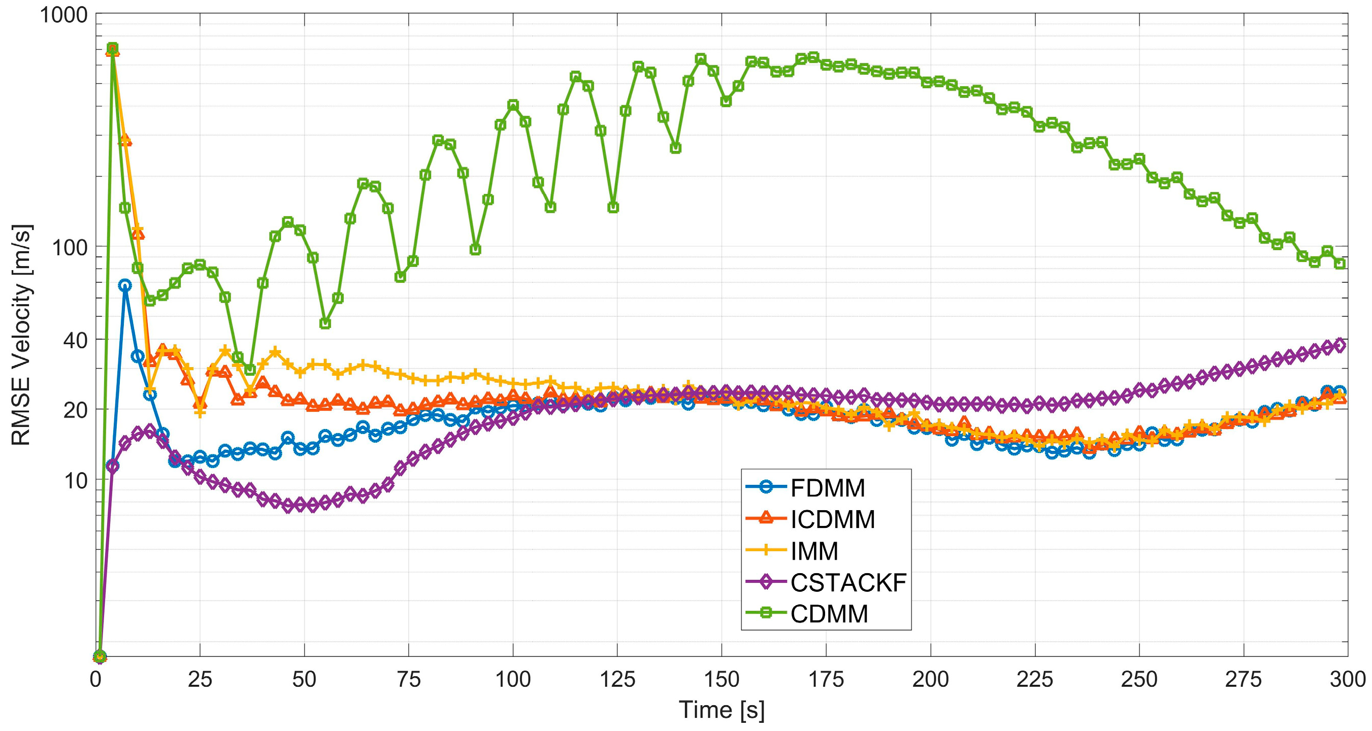
Figure 8.
The average CPU time per period for different algorithms in Case 1.

Figure 9.
The comparison of the estimated trajectories to the true trajectory in one Monte Carlo run in Case 1.
Figure 9.
The comparison of the estimated trajectories to the true trajectory in one Monte Carlo run in Case 1.

Figure 10.
The skip-gliding trajectory of the non-cooperative target.

Figure 11.
The comparison of position RMSE for different algorithms in Case 2.

Figure 12.
The comparison of velocity RMSE for different algorithms in Case 2.

Figure 13.
The average CPU time per period for different algorithms in Case 2.

Figure 14.
The comparison of the estimated trajectories to the true trajectory in one Monte Carlo run in Case 2.
Figure 14.
The comparison of the estimated trajectories to the true trajectory in one Monte Carlo run in Case 2.


Table 1.
The initial orbital parameters of the satellites.
| Parameters | (km) | |||||
|---|---|---|---|---|---|---|
| Satellite 1 | 7,300,000 | 0.000001 | 80.030 | 0 | 0.041 | 345 |
| Satellite 2 | 7,300,000 | 0.000001 | 75.030 | 15 | 0.041 | 345 |
| Satellite 3 | 7,300,000 | 0.000001 | 85.030 | 20 | 0.041 | 345 |
| Satellite 4 | 7,300,000 | 0.000001 | 70.030 | 5 | 0.041 | 345 |
Table 2.
The detailed information of the used models.
| Model | Parameter | Value |
|---|---|---|
| Singer 1 1 | ||
| Singer 2 | 1 | |
| 10 | ||
| 0.01 | ||
| 0.5 | ||
| CV | 2 | 100 |
| CA | 3 | 20 |
1 In the Singer model, refers to the maneuvering frequency; , , and are the design parameters for the different maneuvering modes; 2 refers to the variance of the white noise, ; 3 refers to the power spectral density of the white noise, .
Table 3.
The average tracking error of the total tracking process.
| Algorithm | Average Position Error 1 (m) | Average Velocity Error 2 (m/s) |
|---|---|---|
| FDMM | 35.9289 | 18.0141 |
| ICDMM | 63.5542 | 33.6745 |
| IMM | 70.9382 | 35.9268 |
| CSTACKF | 44.2134 | 19.9188 |
| CDMM | 1119.1594 | 294.4672 |
1 The average position error is the average of over time. 2 The average velocity error is the average of over time.
Table 4.
The average tracking error of the non-cooperative target in the skip-gliding mode.
| Algorithm | Average Position Error 1 (m) | Average Velocity Error 2 (m/s) |
|---|---|---|
| FDMM | 35.7261 | 15.9015 |
| ICDMM | 55.1157 | 29.2621 |
| IMM | 61.2298 | 30.5339 |
| CSTACKF | 56.2843 | 28.8910 |
| CDMM | 919.9887 | 239.1422 |
1 The average position error is the average of over time. 2 The average velocity error is the average of over time.
Publisher’s Note: MDPI stays neutral with regard to jurisdictional claims in published maps and institutional affiliations. |
© 2022 by the authors. Licensee MDPI, Basel, Switzerland. This article is an open access article distributed under the terms and conditions of the Creative Commons Attribution (CC BY) license (https://creativecommons.org/licenses/by/4.0/).
Share and Cite
MDPI and ACS Style
Zhou, F.; Wang, Y.; Zheng, W.; Li, Z.; Wen, X. Fast Distributed Multiple-Model Nonlinearity Estimation for Tracking the Non-Cooperative Highly Maneuvering Target. Remote Sens. 2022, 14, 4239. https://doi.org/10.3390/rs14174239
AMA Style
Zhou F, Wang Y, Zheng W, Li Z, Wen X. Fast Distributed Multiple-Model Nonlinearity Estimation for Tracking the Non-Cooperative Highly Maneuvering Target. Remote Sensing. 2022; 14(17):4239. https://doi.org/10.3390/rs14174239
Chicago/Turabian StyleZhou, Fansen, Yidi Wang, Wei Zheng, Zhao Li, and Xin Wen. 2022. "Fast Distributed Multiple-Model Nonlinearity Estimation for Tracking the Non-Cooperative Highly Maneuvering Target" Remote Sensing 14, no. 17: 4239. https://doi.org/10.3390/rs14174239
Note that from the first issue of 2016, this journal uses article numbers instead of page numbers. See further details here.