Article

Study on the Landscape Space of Typical Mining Areas in Xuzhou City from 2000 to 2020 and Optimization Strategies for Carbon Sink Enhancement

1
Precision Forestry Key Laboratory of Beijing, Beijing Forestry University, Beijing 100083, China
2
Energy Saving & Environmental Protection & Occupational Safety and Health Research Institute, Academy of Railway Sciences Corporation Limited, Beijing 100081, China
*
Author to whom correspondence should be addressed.
Remote Sens. 2022, 14(17), 4185; https://doi.org/10.3390/rs14174185
Submission received: 8 July 2022 / Revised: 11 August 2022 / Accepted: 21 August 2022 / Published: 25 August 2022
(This article belongs to the Special Issue Urban Ecophysiology: A Remote Sensing Perspective)

Abstract

:
The continuous extraction of mining resources has led to the destruction of landscape space, which has had a great impact on the human living environment and pristine ecosystems. Optimizing the ecological spatial networks of mining areas can restore and enhance the damaged ecological environment. However, there are few cases of ecological spatial network optimization in mining areas, and there are still some shortcomings. Therefore, in this study, we propose an ecological spatial network theory and a synergistic enhancement of ecological functions and carbon sink optimization model (SEEC) for urban restoration in mining areas, emphasizing the functional and carbon sink nature of ecological sources. We selected a typical mining area in Xuzhou City as the study area, explored the changes in the nature and function of the ecological spatial network from 2000 to 2020, and selected the ecological spatial network in the mining area of Xuzhou City in 2020 as the optimization study case, adding 27 ecological stepping stones and 72 ecological corridors. Through the comparison of robustness before and after optimization, we found that the optimized ecological spatial network has a stronger stability and ecological restoration ability. This study provides strategies and methods for ecological restoration projects in national mining cities and also provides references and lessons for ecological restoration in other mining areas in the future.

1. Introduction

In recent years, China’s industrialization and urbanization have accelerated [1]. A large number of human actions such as deforestation, surface mining, and sewage discharge have seriously damaged the natural ecosystem [2,3]. Especially in mining cities, long periods of resource extraction and urban expansion have changed the original spatial structure of the landscape [4,5]. Large ecological habitats have been destroyed and replaced by fragmented patches of poor ecological functionality, which weaken the stability and functionality of urban ecosystems and affect the transfer of material and energy information [6,7]. Therefore, the conservation and restoration of urban ecosystems has been a key research issue for a long time [7,8]. In addition, with the reduction in vegetation and ecological degradation, carbon sequestration in urban areas of mining areas has been equally affected by the elevated CO2 emissions, which further aggravates the greenhouse effect and seriously affects the daily lives of human beings [9,10]. However, by means of the monitoring technology of remote sensing, we can obtain information and data of various elements within the ecosystem, monitor and evaluate the ecological environment, and further understand the spatial structure of the landscape and carbon dioxide emissions, while, by combining ecological knowledge, we can further propose strategies to optimize the damaged ecological environment.
China is the largest developing country and CO2 emitter in the world [11]. The Chinese government has proposed to achieve carbon peaking by 2030 and carbon neutrality by 2060 [12]. However, with economic and social development, cities have become a huge source of carbon. Currently, China’s urban CO2 emissions account for 85% of energy consumption [13]. Unlike the carbon emissions of other cities, mining cities generate more CO2 emissions because of their superior coal mining resources and the large number of factories distributed around the mines. In addition, with the large amount of coal mining, the surface of mining cities is fragile and can collapse severely, which also accompanies the further deterioration of the ecological environment and seriously affects the development and transformation of cities [14]. Therefore, it is necessary to propose effective restoration tools for the ecological problems of mining cities.
Vegetation has the functions of water conservation, wind and sand control, and climate regulation, and it is also the best carrier to achieve carbon sequestration [15]. Increasing the amount of regional vegetation or improving the growth environment of regional vegetation can promote plants to perform their physiological functions and promote a virtuous ecological cycle and carbon sequestration [16]. In fact, plant population and growth depend on various environmental factors, such as humidity and temperature, soil microbial communities, hormones, etc., and these microscopic ecological elements are usually restricted in a more macroscopic spatial pattern [17]. A well-formed ecological energy cycle process can enhance ecological elements and ultimately improve the growth environment of vegetation. For mining cities with severe landscape fragmentation, their ecological energy and material cycles are severely hindered. Therefore, we can build protective ecological corridors to build a conducive path for energy transfer and connect the fragmented ecological sources to form an organic urban ecosystem. In addition, we can set up a certain number of ecological stepping stones to further enhance the communication and circulation of energy between the sources [18,19].
In order to protect the landscape space to a greater extent and realize a good way of material and energy transmission, we can construct an ecological spatial network [20]. An ecological spatial network is an ecological method that combines the original ecological network theory with the complex network theory [21]. At present, the primitive ecological network theory has formed a more complete theoretical system to identify ecological sources through ecological sensitivity evaluation, the ecological safety model, patch connectivity and other forms of evaluation systems, and to construct ecological corridors through the minimum cumulative resistance model (MCR) [22,23]. The spatial structure of the landscape in the study area can be initially formed through the original ecological network, yet this structure lacks quantitative indicators to explain the relationship between landscape elements. However, by combining complex network theory and using topological indicators, the role of each ecological element in the network can be better determined, the ecological network can be quantified and simplified, and an optimization scheme can be proposed based on the values in the topological indicators [24]. At present, the research on ecological spatial networks is still in the initial stage; some scholars simulate the ecological safety problem in the desert oasis area, and some scholars study the biodiversity, but most of them only construct the ecological spatial network in a certain year [17,25]. In addition, there are few cases that explore the ecological and carbon sink problems at an urban scale. In fact, the mining and destruction process of mining areas is time-series in nature, so we need to construct a time-series ecological spatial network to fully reflect the ecological spatial pattern and carbon sink change process.
The purpose of this paper is to study the changes in landscape spatial structure and function in typical mining areas in Xuzhou City during 2000–2020 and the strategies to enhance carbon sinks. Through the ecological construction of the country, the original ecological space is restored, and theoretical and methodological support is provided for future ecological restoration projects in mining cities. In this study, we propose the SEEC optimization model to optimize and enhance the nodes with weak functionality and carbon sink in the landscape space. We simulate ecological perturbations by malicious and random attacks, and finally we evaluate the optimization results of the model by comparing the robustness before and after optimization.

2. Materials and Methods
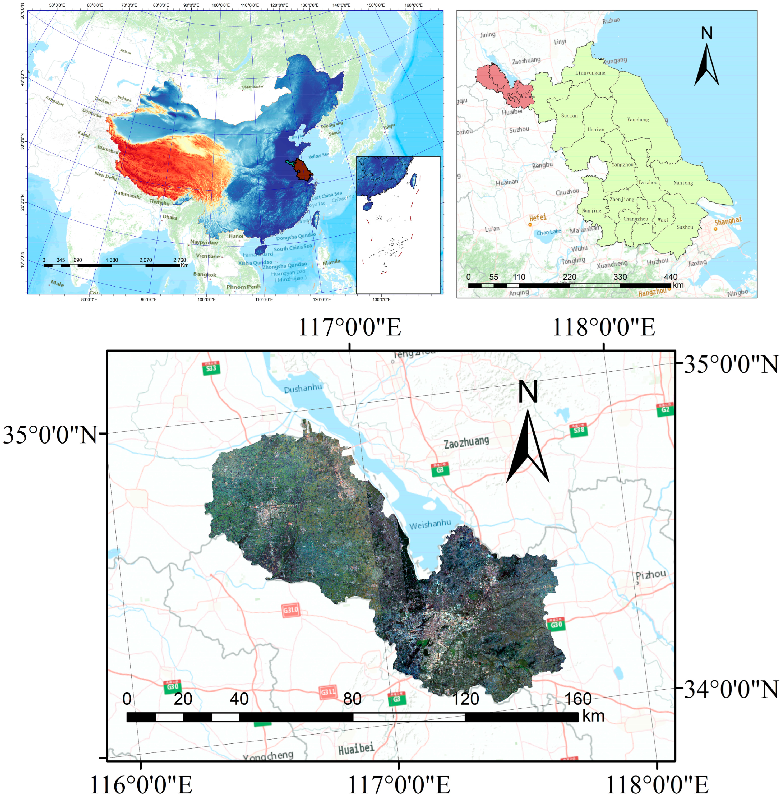
2.1. Study Area

The study area is located in the mining area of Xuzhou City, Jiangsu Province, in the northwestern part of Xuzhou City (Figure 1). The topography of the study area is high in the west and low in the east, dominated by plains and hills and is a transition zone from subtropical monsoon climate to warm temperate monsoon climate zone, with annual sunshine hours from 2284 to 2495, sunshine rate from 52% to 57%, annual temperature of 14.9 °C, and average annual precipitation from 800 to 930 mm. The study area is rich in mineral resources and is an important coal producing area in China. The study area involves four key mining areas in Xuzhou City, which are the key mining area for rock salt in Feng County, the key mining area for coal in Peixian County, the key mining area for limestone for cement in Tongshan District, and the key mining area for limestone for cement in Jiawang District.

2.2. Data Sources and Processing

Multiple datasets from 2000 to 2020 were used in this study (Figure 2). (1) Road network and water network data were obtained from OpenStreetMap (https://www.openstreetmap.org/, accessed on 7 July 2022), and we obtained the road network density and water network density by density analysis in Arcgis. (2) DEM and land use data were obtained from the Resource and Environment Science and Data Center of Chinese Academy of Sciences (https://www.resdc.cn/, accessed on 7 July 2022), and we obtained the study area data by Arcgis clipping. (3) Slope data were obtained from the Geographical Detection Cloud Platform (http://www.dsac.cn/DataProduct/Index/2010, accessed on 7 July 2022). We obtained the data of the study area by Arcgis cropping. (4) NDVI and MNDWI data were obtained from Google Earth Engine data analysis platform (https://earthengine.google.com/, accessed on 7 July 2022). We obtained the study area data by Arcgis cropping [26,27]. (5) population density data from WorldPop (https://www.worldpop.org/, accessed on 7 July 2022), (6) nighttime light data from Harvard dataverse (https://dataverse.harvard.edu/, accessed on 7 July 2022). We obtained the study area data by Arcgis cropping.

3. Methods

The research method of this paper is divided into 3 parts (Figure 3). The first part is the construction of ecological spatial network, and we screened ecological sources by landscape morphological spatial pattern analysis method (MSPA). We used nighttime lighting data and energy factors to modify the original MCR model, and by combining the eight ecological resistance factors of DEM, SLOPE, NDVI, MNDWI, LUCC, population density, water network density, road network density from 2000 to 2020. The minimum ecological cumulative resistance surface and ecological corridors were calculated from 2000 to 2020, and the changes in the minimum ecological cumulative resistance surface were analyzed. The second part is the construction of SEEC optimization model. We comprehensively considered the functionality and carbon sink of ecological sources and screened out the weak functional nodes and weak carbon sink nodes and proposed the optimization strategy by calculating the node topology values and Pearson correlation analysis. The third part is the validation part. We verified the effect of optimization by calculating and comparing the robustness of ecological spatial network before and after optimization.

3.1. Construction of Ecological Space Network

Ecological space network is an application of ecological network theory and complex network theory in landscape ecology. Using complex network theory, ecological sources and ecological corridors can be abstracted as nodes and edges of a network. In fact, many observed networks have properties corresponding to the undirected, small-world network type. While primitive ecological networks are usually used as a static network form, actual networks are characterized by a large number of dynamic ecological processes such as energy and material information exchange, which can be better described by the topological indicators of complex network theory, as well as further understanding of the inherent structure and information of the network.

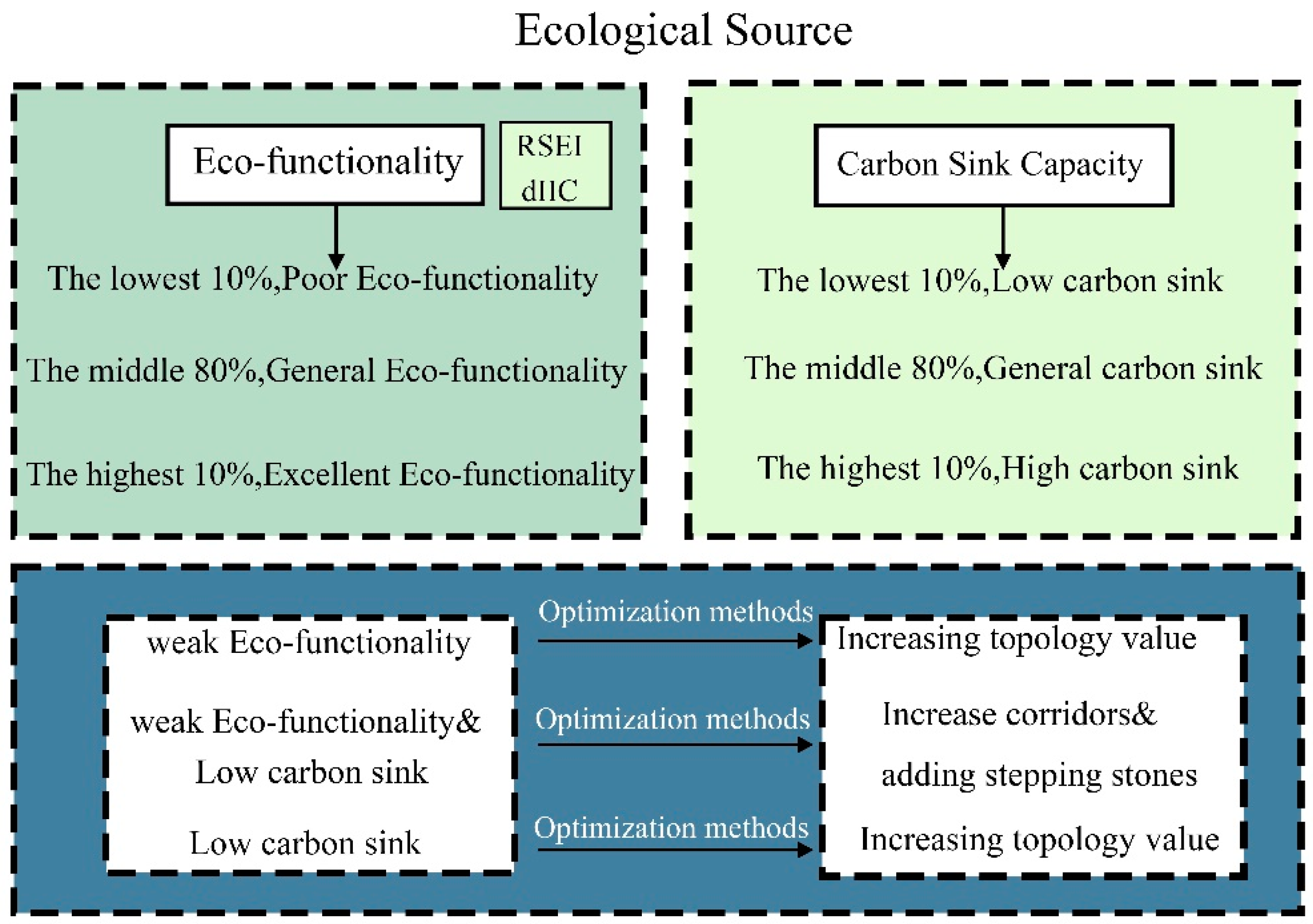
3.1.1. Ecological Sources Identification Based on MSPA Analysis

Morphological spatial pattern analysis (MSPA) is an image processing method to measure, identify and segment the space of raster images based on mathematical morphological principles such as expansion, open operation, and closed operation, which can better identify important habitat patches in the study area and obtain core area patches by erosion calculation, and after a series of mathematical operations such as expansion reconstruction and skeleton extraction, we obtained core. We obtained seven types of patches, including core, islet, edge, perforation, bridge, loop, and branch [28,29]. We used the eight-neighborhood method to extract the core area larger than 0.2 km as the ecological source area and classify the ecological source area into four types according to the ecological function and carbon sink capacity: forest, shrub, grassland, and water.

3.1.2. Ecological Corridor Construction Based on the Modified MCR Model

Ecological corridors can connect different ecological sources and provide channels for the exchange of energy and materials between sources [30,31]. The traditional method of extracting ecological corridors is obtained by constructing the minimum resistance model (MCR), which is calculated in Arcgis using cost paths and cost distances [32]. However, the original MCR model ignores the hindering effect of humans on the landscape under different development intensities in different land types, and also the process of ecological energy flow is hindered differently in different locations. Therefore, we revised the original MCR model as follows.
V MCR = f min i = 1 , j = 1 i = m , m = j ( D ij R i N j P j )
where V MCR is the face value of the minimum ecological cumulative resistance of the modified ecological land. f min is the minimum value of cumulative resistance of a land unit. D ij is the spatial distance from ecological sources j to land unit i. R i is the resistance coefficient of the movement process of land unit i. N j is the radiation value of nighttime light data in ecological sources j. P j is the energy factor of ecological sources j, the larger the value indicates the greater the ecological energy of the ecological source patch, where the energy factor P j is calculated by the formula
P j = A j N j  
where A j is the area of the j ecological source land patch, N j is the r normalized index of the j ecological land patch, NDVI and MNDWI were selected as normalized indices in this study, so r was taken as 1 and 2.
In addition, we graded the eight resistance factors according to the natural breakpoint method, determined the weights of each factor using the entropy value method, and accumulated all the factors in a graded manner to obtain a comprehensive resistance surface, and the gradation of resistance values is shown in Table S1.

3.2. Ecological Stepping Stones

Ecological stepping stones are a series of small patches located between large ecological patches [33]. Unlike other fragmented ecological patches, ecological stepping stones have stronger connectivity and stability, which can better connect and transfer material energy. In the context of serious ecological deterioration in mining cities, ecological stepping stones are a good application for urban stock ecological space. Therefore, we chose to add ecological stepping stones in areas with long ecological corridors, and we also used the patch shape index to screen ecological stepping stones. In ecology, the simpler the shape of the patches, the less they are subject to human activity intervention, and the higher the stability of the patches
LSI = E 2 π A
where E is the total length of all patch boundaries in the landscape and A is the total area of the landscape.

3.3. Topological Indicators for Evaluating Ecological Spatial Networks

Topological indicators of ecological spatial networks are a way to quantify the structure and function of the network [34,35]. In this study, nine topological indicators of degree, average path length, clustering coefficient, proximity centrality, meso-centrality, eigenvector centrality, modularity, Integral Index of Connectivity (dIIC), and Remote Sensing Ecological Index (RSEI) were used to describe the ecological spatial network. The different metrics are defined in Supplementary Materials.

3.4. SEEC Optimization Model

Ecological connectivity has been the key indicator for evaluating ecological sources; however, we believe that in addition to connectivity, the ecological values of the ecological sources themselves are equally important, so we introduced RSEI as an indicator for evaluating the inherent ecological attributes of ecological sources. We combined the two indicators and thus evaluated ecological sources comprehensively. In addition, for mining cities, as well as ecological issues, the carbon sink capacity of ecological sources is equally important, so we calculated the carbon sink value of each ecological source site through the carbon sink formula, and then evaluated the carbon sink capacity of ecological sources. Through the SEEC model, we obtained three types of weak ecological sources: sources with weak ecological function, sources with weak carbon sink function, and sources with both weak ecological and carbon sink capacity. We followed different strategies to optimize and enhance the three types of sources (Figure 4). Among them, the carbon sink equation is as follows:
C t = i = 1 n A i S i
where C t is the total amount of carbon sink. i is the land use type. A is the land area. S is the carbon sink coefficient. The carbon sink coefficients are determined from the existing domestic and international literature, as shown in Table 1.

4. Result

4.1. Ecological Spatial Network Construction in the Study Area from 2000 to 2020

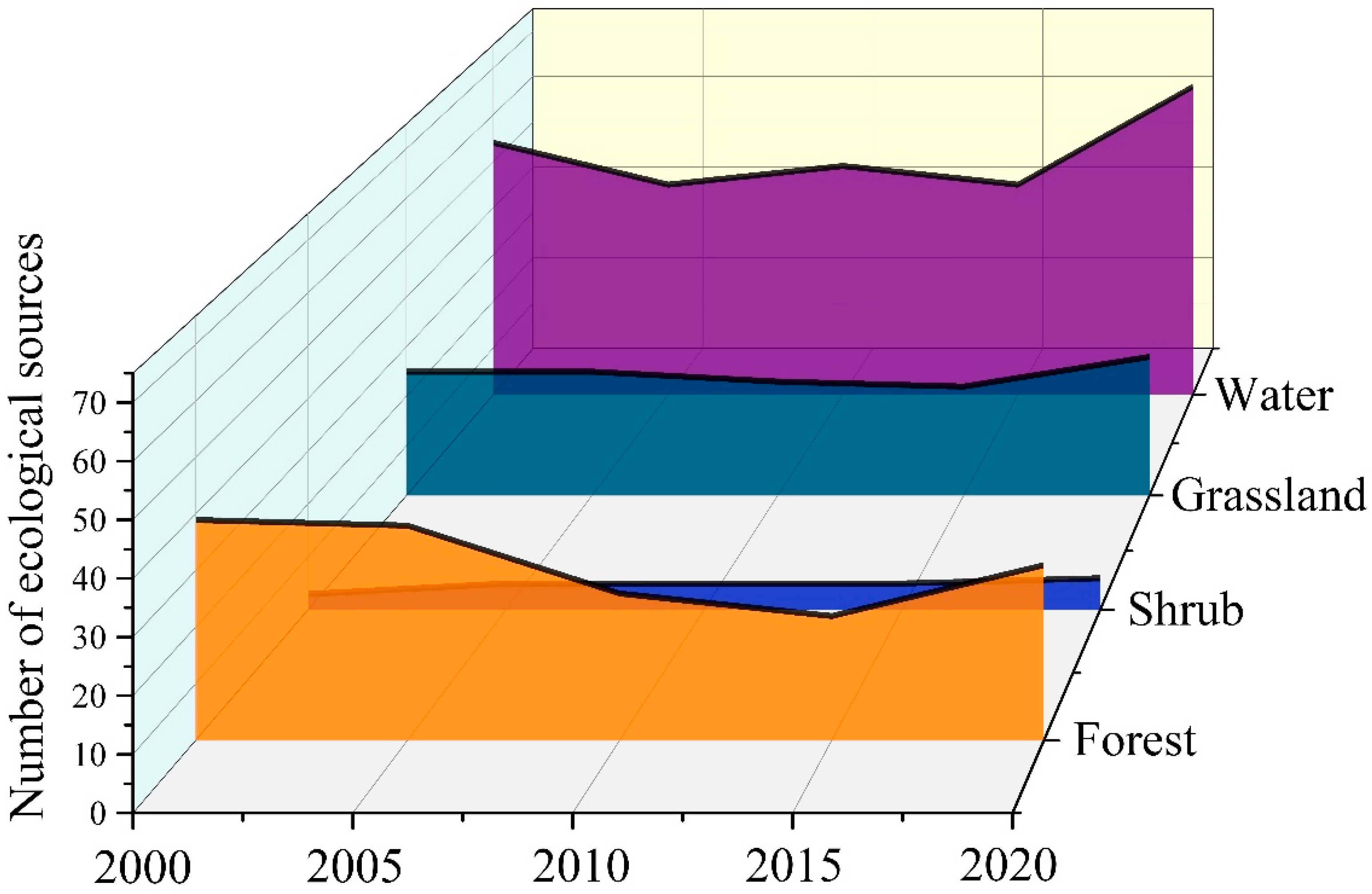
4.1.1. Extraction and Classification of Ecological Sources in the Study Area from 2000 to 2020

According to the actual situation of the study area, we identified forests, shrubs, grasslands, and water bodies in the core area patches with an area larger than 0.2 km2 as ecological sources. We finally obtained 121 ecological sources in 2000, 113 ecological sources in 2005, 103 ecological sources in 2010, 94 ecological sources in 2015, and 131 ecological sources in 2020, and we found that the number of ecological sources showed a decreasing trend year by year between 2000 and 2015, which indicates that the study area may have been damaged by anthropogenic damage such as surface mining, the quality of the ecological environment is not added, and the number of sources decreases. However, in 2020, the number of ecological sources reached the highest value in all of the years, which indicates that the government has paid more attention to the protection of the ecological environment and the ecological restoration project has achieved a certain effect. In addition, the changes in the number of different types of ecological sources are shown in Figure 5. We found that the number of forest ecological sources, grassland ecological sources, and water ecological sources showed a decreasing trend during 2000–2015, while the number of shrub ecological sources remained stable. Between 2015 and 2020, the number of all types of ecological sources increased to some extent.

4.1.2. Minimum Cumulative Ecological Resistance Surface Analysis for 2000–2020

We found that the minimum cumulative ecological resistance surface in the study area showed an increasing trend from 2000 to 2020, and the resistance value showed a large increase from 2005 to 2010, and nearly the same value from 2010 to 2015, indicating a good ecological control during this period (Figure 6). This indicates that although the number of ecological sources has increased, they are not performing as ecologically effective as they should, and therefore an in-depth understanding of the spatial function and structure of the landscape in the study area is still needed. In addition, we found that the areas with higher resistance values each year are almost located in the same geospatial location (Peixian and Fengxian), probably due to the fact that the area has a key rock salt mining area in Fengxian and a key coal mining area in Peixian, Xuzhou, and thus has a poor ecological environment and higher ecological resistance.

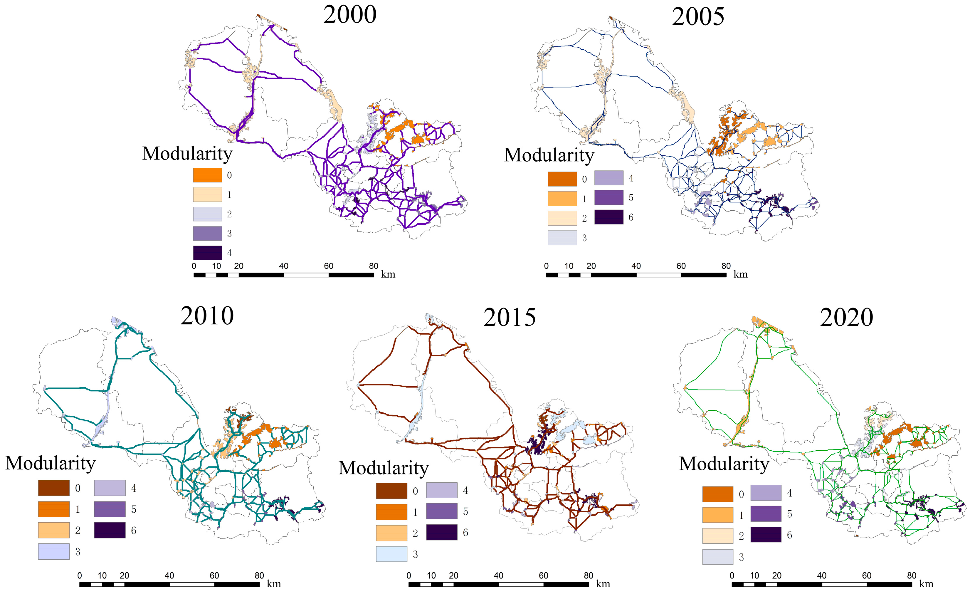
4.1.3. Ecological Spatial Network Analysis 2000–2020

We generated the ecological corridors of the ecological spatial network from 2000 to 2020 by the cost path model in Arcgis. We extracted 290 ecological corridors in 2000, 276 ecological corridors in 2005, 251 ecological corridors in 2010, 227 ecological corridors in 2015, and 333 ecological corridors in 2020, and the number of ecological corridors showed an overall trend of first decreasing and then increasing, and this change was the same as the trend of the number of ecological sources. In addition, we found that the number of ecological corridors and ecological sources in the western part of the study area is smaller and the length of ecological corridors is longer, and the distribution of ecological sources is sparse, while the ecological corridors in the eastern part are shorter and the distribution of ecological sources is dense (Figure 7). This indicates that the ecological localities in the western region are poor and the spatial pattern of the landscape needs to be optimized and enhanced.
We also found that the spatial pattern of the landscape in the study area showed a community-like distribution form, and we assigned the calculated modularity index to the ecological sources to obtain the zoning of the modularity of the ecological sources (Figure 8). We found that the ecological spatial network was divided into six communities in all of the years except 2000, which indicated that the landscape heterogeneity among ecological sources was more obvious in 2005–2020, and the differences among different community networks were more obvious. According to the definition of modularity, ecological nodes with the same modularity possess stronger connectivity and resilience in the face of anthropogenic disturbance, and natural aggression. In addition, we also found that the classification of community networks was correlated with geospatial location, and ecological nodes with the same modularity were located similarly in geospatial space. We speculate that this may be related to natural factors such as humidity, temperature, sunshine duration, and rainfall because natural factors have similar properties in similar geospatial spaces, duration, and rainfall.

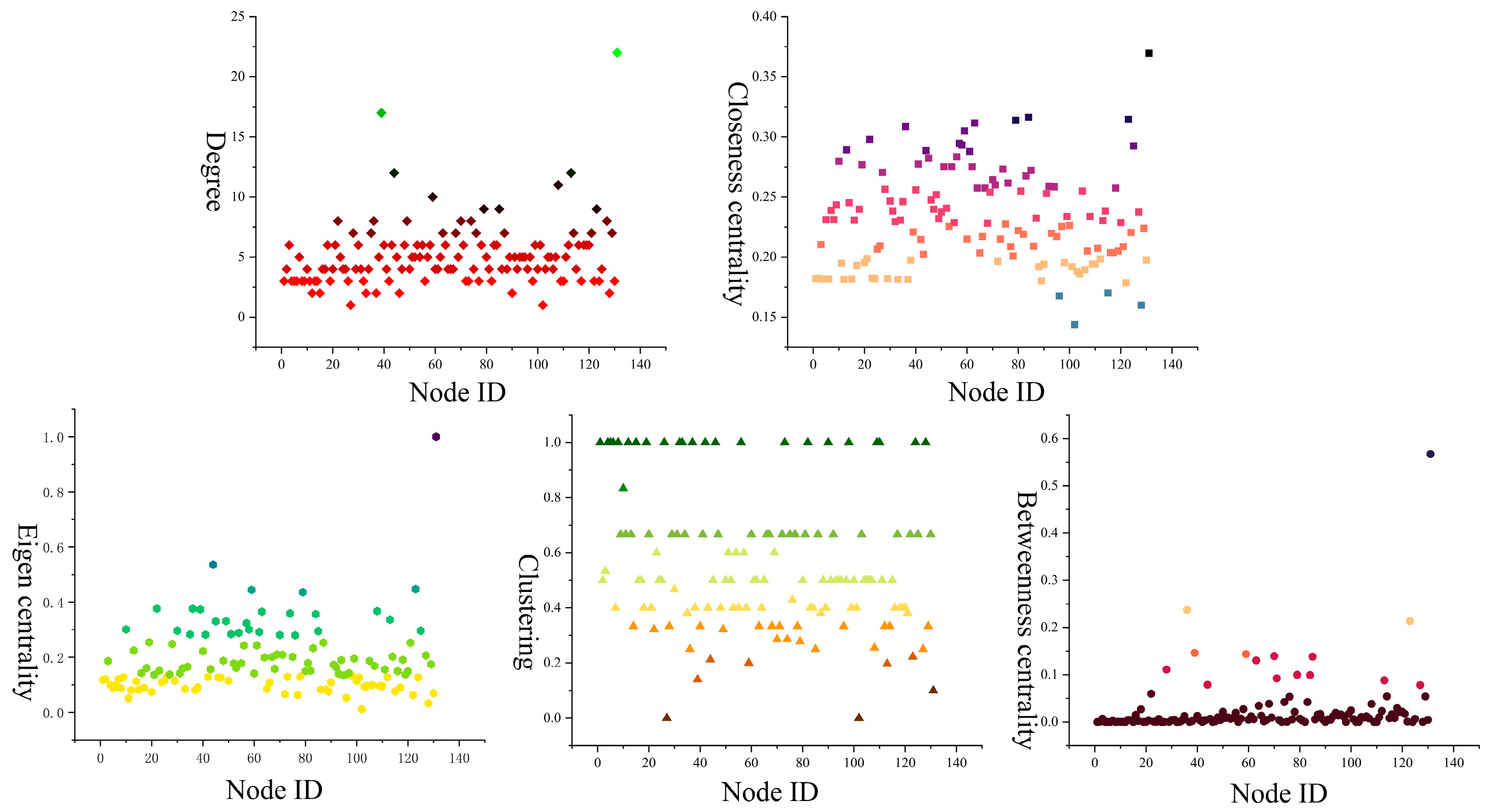
4.2. Average Network Topology Metrics Analysis 2000–2020

We calculated the average topological values of the ecological spatial network for 2000–2020 as shown in Table 2. We find that degree shows an increasing trend, which indicates that the importance of ecological nodes has been enhanced in 2000–2020. Betweenness centrality and eigen centrality show a decreasing trend, which indicates that the energy and information transfer ability between ecological nodes is weakened and the connectivity of ecological nodes is reduced. In addition, closeness centrality and clustering showed little change and remained basically stable.

4.3. SEEC Optimization Enhancement

We selected the ecological spatial network of the study area in 2020 as a case of optimization and enhancement and identified the 10% nodes with the lowest ecological functionality as weak ecological functionality nodes and the 10% nodes with the lowest carbon sink values as weak carbon sink nodes. Finally, we extracted 10 nodes with weak ecological functionality only, 7 nodes with weak carbon sink only, and 3 nodes with weak ecological functionality and weak carbon sink. We proposed the strategy of increasing ecological corridors and ecological stepping stones for the weak ecological function nodes, and the strategy of improving betweeness centrality for the weak carbon sink nodes.

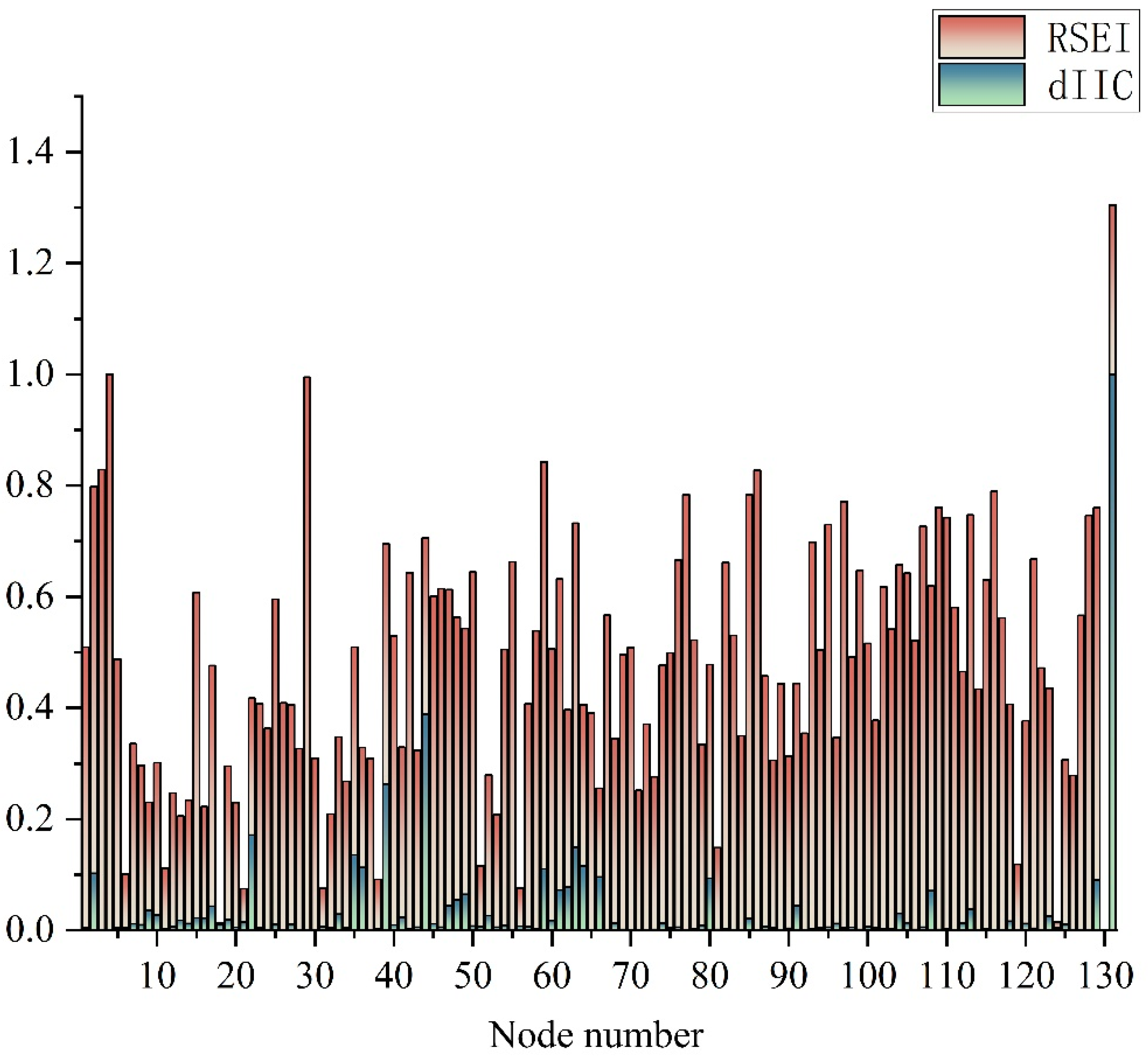
4.3.1. 2020 Carbon Sink Relevance Analysis

We calculated the carbon sink value of each ecological source site and constructed the relationship between carbon sink and topological indicators by Pearson correlation analysis. We found that the betweeness centrality of shrubs, grasslands, and water showed highly significant positive correlation and significant positive correlation with carbon sinks (Figure 9). Therefore, we identified the 10% nodes with the lowest carbon sink values in shrubs, grasslands, and water bodies as the weak carbon sink nodes: 10 nodes in total. Increasing the betweeness centrality of these nodes will improve the carbon sink of ecological sources.

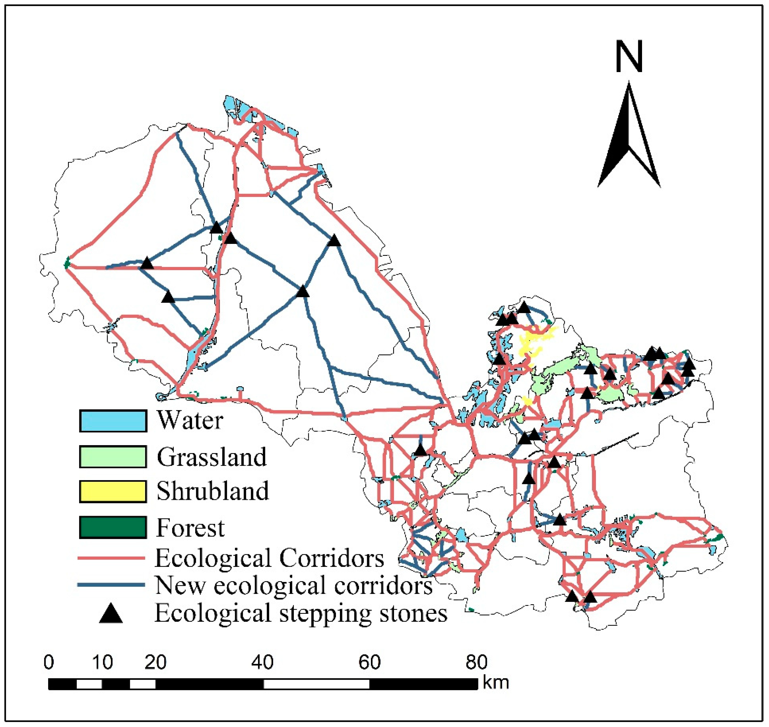
4.3.2. Optimization and Enhancement of Ecological Spatial Network in Xuzhou Mining Area

We identified 10 ecologically weak nodes (6, 11, 13, 18, 21, 31, 38, 51, 56, 124) and 7 carbon sink weak nodes (5, 32, 69, 88, 93, 101, 115) through the SEEC model, and 3 ecologically weak nodes (81, 119, 130). For the nodes with weak ecological functionality, we proposed to increase the ecological corridors and ecological stepping stones, and for the nodes with weak carbon sinks, we proposed to increase the shortest paths of the nodes to improve their Betweenness Centrality. For nodes with both weaknesses, we adopted both of these policies. We selected the areas around the weak nodes, screened the ecological stepping stones by the landscape patch shape index, and obtained the new ecological spatial network by the original integrated cumulative resistance surface, and finally we added 27 ecological stepping stones and 72 ecological corridors(Figure 10). We found that the ecological sources in the northwestern part of the study area were better connected in the new ecological spatial network, and the ecological corridors around the weak nodes were increased.

4.3.3. Comparison of Network Robustness before and after Optimization

We used random attacks to simulate natural disasters such as fires, pests, and earthquakes in the landscape space, and malicious attacks to simulate man-made disasters such as deforestation and water pollution in the landscape space, and finally we evaluated the optimization results by the performance of the robustness before and after optimization. In this study, we chose three kinds of robustness: the recovery robustness of the nodes, recovery robustness of edges, and connection robustness(Figure 11).
In the recovery robustness of the nodes, we found that the robustness of the optimized ecospatial network decreased significantly slower than that of the pre-optimized network in random attacks. The network before and after optimization maintained high values above 0.9 after attacking 89,105 nodes, respectively, and after attacking 129,152 nodes, the network robustness fell below 0.1 and the network eventually collapsed. We found that the robustness of the network before optimization was below 0.1 when 126 nodes were maliciously attacked and the network crashed; however, the robustness of the network after optimization was still maintained at a high value until 156 nodes were attacked and the network robustness was below 0.1. In the recovery robustness of edges, we found that the network robustness before and after optimization was below 0.1. We found that the network robustness improved slightly but not significantly before and after the optimization, especially in the initial attack when the network robustness started to decrease before the optimization, but the network robustness still maintained a high value after the optimization; however, the robustness decreased at about the same rate in the subsequent attacks. In connection robustness, we found that the robustness of the network was significantly enhanced, and unlike the first two forms of network robustness decline, connection robustness showed a wave-like decline. We found that the stability of the network was significantly improved in both malicious and random attacks. When 42 nodes were maliciously attacked, the pre-optimization network robustness was below 0.1 and the network crashed, while the post-optimization network robustness was only below 0.1 after 84 nodes were maliciously attacked. In the random attack, the pre-optimization network robustness decreased rapidly with the increase in attacked nodes, while the post-optimization network still maintained a high robustness and decreased slowly. In addition, we also found that the network robustness kept trying to recover during the random attack, and the pre-optimized network only recovered to 0.29, while the optimized network recovered up to 0.4. Combining the performance of the three types of robustness, we believe that the stability and ecological recovery of the optimized ecological space network were improved.

5. Discussion

5.1. Topological Properties of the Ecological Spatial Network in 2020

We used Gephi to obtain the values of each topological index of the ecological spatial network in 2020 (Figure 12). We found a total of six nodes with a degree greater than 10, namely, nodes 131, 39, 44, 113, 108, and 59, which indicates that these nodes have a high degree of influence in the network and have multiple nodes connected to them, with node 131 reaching a maximum degree of 22. A total of nine nodes were found with a degree less than 3: nodes 27, 102, 12, 33, 37, 90, 15, 46 and 128, of which 27 and 102 have the lowest degree of 1. The seven nodes with a closeness centrality greater than 0.3 are 131, 84, 123, 79, 63, 36, and 59, of which 131 has a maximum closeness centrality of 0.37, which indicates that these nodes are closer to the center of the network. There are five nodes with a closeness centrality lower than 0.18: 102, 128, 96, 115, and 122, of which 102 has the lowest closeness centrality value of 0.144. Betweeness centrality is higher than 0.2. The nodes with a betweeness centrality higher than 0.2 are 131, 36, and 123, and the highest value of betweeness centrality is 0.567211, which indicates that this node has the strongest ability for information and energy transfer. Twenty-five nodes have a betweeness centrality of 0.23. There are 23 nodes with clustering of 1 and 2 nodes with clustering of 0, which are nodes 102 and 27, indicating that these nodes are poorly aggregated and their stability is poor and easily destroyed. The node with an eigen centrality of 1 is node 131, which is significantly higher than other nodes, indicating that the node’s proximity nodes are of high importance, and there are two nodes below 0.05.
We extracted and obtained the RSEI and dIIC of each ecological source site, and normalized the two indicators separately and then summed them, and the results are shown in Figure 13. We found that the normalized dIIC of node 131 was 1, which was significantly higher than the other nodes, indicating that node 131 had the strongest connectivity, and the normalized dIIC of node 71 was 0, which required additional ecological corridors to enhance its connectivity. We also found that the nodes with an RSEI higher than 0.8 were 4, 29, 3, and 86, indicating that the ecological quality of these nodes was higher, and the RSEI of node 4 reached the highest value of 1. The eight nodes with an RSEI lower than 0.1 were nodes 130, 18, 124, 21, 56, 31, 38, and 6, which had a poor ecological background and needed to be enhanced. By calculating the superimposed values of the RSEI and dIIC, we found that nodes 131, 4, 29, 59, 3, and 86 were at higher values, indicating that these nodes are more functional, with node 131 having the highest value. There were seven nodes with superposition values lower than 0.1, namely, nodes 130, 18, 124, 21, 31, 56, and 38.
Combining the topology values, we found that node 123 performed better in the complex network topology metrics, with higher values in closeness centrality and betweeness centrality, while nodes 102 and 128 had lower values in closeness centrality, clustering and eigen centrality. In addition, nodes 131 and 59 had high values in the complex network topology index and ecological functional coupling index, especially node 131, which had the highest value in all types of topology index. Therefore, focusing on the protection of these two ecological nodes is beneficial to the conservation of ecological functions and structures in the study area.

5.2. Dynamic Variability of Landscape Patterns

With the continuous expansion of cities and resource extraction, the landscape ecological issues of mining cities have become increasingly important [40]. In order to further explore the impact of mining on the urban ecological space, we introduced a landscape pattern index for the study of temporal changes (Figure 14). With FRAGSTATS software, we selected total landscape area (TA), largest patch index (LPI), landscape shape index (LSI), fractal dimension (PAFRAC), spread index (CONTAG), separation (SPLIT), Shannon diversity index (SHDI), Shannon evenness index (SHEI), and their meanings are shown in Table S2.
We found that the TA varied greatly over 20 years, but remained stable in general, which indicates that the overall landscape area was destroyed, but Xuzhou City has taken effective measures to restore the destroyed landscape area. An increasing trend was shown in 2020. SPLIT increased year by year and reached the highest value in 2020, which indicates the increasing fragmentation of the landscape, and PAFRAC showed a wave-like increasing trend, which indicates the decreasing stability of the landscape patches.
We found that although Xuzhou City has taken certain ecological restoration measures to ensure that the number of patches in the landscape space remains stable, there is still no solution to the increasing intensity of human interference with the landscape space, as evidenced by the comprehensive cumulative resistance surface from 2000 to 2020. As the intensity of development increases, this also aggravates the fragmentation of patches in the ecological space, and the stability of patches gradually decreases. Therefore, this tells us that merely increasing the number of sources cannot improve the ecological environment and ecological functions of the Xuzhou mining area, and we still need to further understand its intrinsic structure and characteristics by constructing an ecological spatial network in order to propose a more scientific and accurate optimization strategy.

5.3. Advantages of SEEC Model for Urban Ecological Optimization in Mining Areas

In the current screening of ecological sources, many studies only consider the connectivity of ecological sources (dIIC) and ignore the ecological quality of the sources [41,42]. We believe that in addition to the connectivity function of ecological sources with other ecological sources, their inherent ecological properties should also be valued, so we introduced the RSEI evaluation index in the SEEC model to further screen ecological sources. In addition, we believe that the measures and tools adopted in the optimization process should be different for different ecological problems, but, unfortunately, in the current optimization studies, the tools used are usually to improve the connectivity of ecological sources, and this optimization approach lacks the specificity of solving different ecological problems, and the optimization improvement effect is not significant. As a result, a large amount of resources may be wasted in the implementation of ecological restoration projects. The SEEC model in this study focuses on the restoration of ecological problems in mining areas. In addition to solving the fragmentation of ecological sources, we also consider the carbon sequestration capacity of the mining landscape space and propose an optimization strategy to improve carbon sinks in response to the high carbon emission problem in mining areas, so the SEEC model is more typical and specific for restoring mining areas.

5.4. Advantages of Building a Time-Series Ecological Spatial Network

Human resource extraction for mining areas has always been a behavioral process with temporal characteristics. As the intensity of exploitation increases, the topological nature and function of the ecological spatial network will inevitably change as well. Therefore, a dynamic perspective should be adopted to explore the ecological spatial structure of mining areas. However, most studies have only examined the ecological network for a particular year, which leads to there being insufficient knowledge about the ecological spatial network in mining areas [43,44]. Therefore, we constructed an ecological spatial network of the Xuzhou mining area from 2000 to 2020 to fully explore the ecological functions and nature of the network. In addition, the ecological spatial network is different from the original ecological network. We introduced the complex network theory on top of the ecological network. In fact, ecological sources and ecological corridors exhibit different ecological functions and ecological roles in different geographic spaces, yet the original ecological network lacks quantitative indicators for the functions of different sources and corridors. Through the topological indicators of complex networks, we can further explore the nature of ecological networks and propose optimization strategies.

5.5. Limitations and Prospects

Ecospatial networks help us to understand the structural characteristics of landscape spaces while enabling the conservation and regional development of landscape spaces [45]. However, there are still some limitations of ecospatial networks. Firstly, the ecological spatial network is still in the theoretical stage, and the effect of optimization needs to be further determined by the government after a long period of ecological engineering construction. Secondly, the ecological network is mainly constructed to achieve ecological restoration, but it lacks the influence of socio-economic factors. The construction of ecological corridors requires a lot of human and physical economic costs, so how to weigh the economic costs spent and the ecological benefits obtained is worth further study. Finally, there is no internationally accepted standard for the selection of ecological resistance factors, which inevitably leads to the formation of different ecological networks in the same study area due to the adoption of different resistance factors. To some extent, the ecological network theory still needs further improvement and unification.

6. Conclusions

In this study, we constructed the ecological spatial network of the Xuzhou mining area from 2000 to 2020, and analyzed the changes in ecological spatial network function, nature, and resistance surface during 20 years by combining complex network theory. In addition, we selected the ecological spatial network in 2020 and obtained 10 nodes with weak ecological functionality only, 7 nodes with weak carbon sink only, and 3 nodes with weak ecological functionality and weak carbon sink by screening through the SEEC model. Through Pearson correlation coefficient analysis, we found that carbon sequestration showed a highly significant and significant positive correlation with the betweeness centrality of shrub, grassland, and water ecological nodes. Finally, we added 27 ecological stepping stones and 72 ecological corridors and found that the robustness of the optimized ecological spatial network was better than that of the pre-optimized network.
Nowadays, the international community is highly focused on carbon emission and carbon sequestration, and mining cities as a huge carbon source have great potential to enhance the ecological environment and carbon sequestration. However, without human intervention, measures to close coal mines can lead to long and slow ecological restoration cycles. Therefore, we can enhance the natural ecological background and reduce the ecological restoration cycle by adding ecological stepping stones and ecological corridors to facilitate the transfer of energy and material information through ecological restoration projects. At present, in the context of ecological restoration construction in China, ecological restoration planning in mining cities has a certain necessity. In this study, a typical mining area in Xuzhou City is selected for optimization and enhancement to provide a reference for ecological restoration projects in mining areas in Xuzhou City and other mining areas.

Supplementary Materials

The following supporting information can be downloaded at: https://www.mdpi.com/article/10.3390/rs14174185/s1, Table S1. Evaluation factors of ecological resistance; Definition of topology indicators; Table S2. Landscape Pattern Index Definition.

Author Contributions

Conceptualization, S.Q., Q.Y., T.N. and M.F.; Methodology, S.Q., Q.Y. and H.G.; Software, S.L.; Supervision, H.L.; Writing—original draft, S.Q. All authors have read and agreed to the published version of the manuscript.

Funding

This work was supported by the Youth Science Foundation of National Natural Science Foundation of China (No. 42001211).

Data Availability Statement

Publicly available datasets were analyzed in this study. The data sources and access links are indicated in the text.

Conflicts of Interest

The authors declare no conflict of interest.

References

  1. Shi, Y.; Feng, C.-C.; Yu, Q.; Han, R.; Guo, L. Contradiction or coordination? The spatiotemporal relationship between landscape ecological risks and urbanization from coupling perspectives in China. J. Clean. Prod. 2022, 363, 132557. [Google Scholar] [CrossRef]
  2. Wang, Z.; Liang, L.; Sun, Z.; Wang, X. Spatiotemporal differentiation and the factors influencing urbanization and ecological environment synergistic effects within the Beijing-Tianjin-Hebei urban agglomeration. J. Environ. Manag. 2019, 243, 227–239. [Google Scholar] [CrossRef]
  3. Zou, C.; Zhu, J.; Lou, K.; Yang, L. Coupling coordination and spatiotemporal heterogeneity between urbanization and ecological environment in Shaanxi Province, China. Ecol. Indic. 2022, 141, 109152. [Google Scholar] [CrossRef]
  4. Wu, J.; Zhu, Q.; Qiao, N.; Wang, Z.; Sha, W.; Luo, K.; Wang, H.; Feng, Z. Ecological risk assessment of coal mine area based on “source-sink” landscape theory—A case study of Pingshuo mining area. J. Clean. Prod. 2021, 295, 126371. [Google Scholar] [CrossRef]
  5. Wu, Z.; Lei, S.; Yan, Q.; Bian, Z.; Lu, Q. Landscape ecological network construction controlling surface coal mining effect on landscape ecology: A case study of a mining city in semi-arid steppe. Ecol. Indic. 2021, 133, 108403. [Google Scholar] [CrossRef]
  6. Osman, A.; Mariwah, S.; Yawson, D.O.; Atampugre, G. Changing land cover and small mammal habitats: Implications for landscape ecological integrity. Environ. Chall. 2022, 7, 100514. [Google Scholar] [CrossRef]
  7. Wei, Y.; Song, B.; Wang, Y. Designing cross-region ecological compensation scheme by integrating habitat maintenance services production and consumption—A case study of Jing-Jin-Ji region. J. Environ. Manag. 2022, 311, 114820. [Google Scholar] [CrossRef]
  8. Song, W.; Feng, Y.; Wang, Z. Ecological restoration programs dominate vegetation greening in China. Sci. Total Environ. 2022, 848, 157729. [Google Scholar] [CrossRef]
  9. Lv, T.; Hu, H.; Zhang, X.; Wang, L.; Fu, S. Impact of multidimensional urbanization on carbon emissions in an ecological civilization experimental area of China. Phys. Chem. Earth Parts A/B/C 2022, 126, 103120. [Google Scholar] [CrossRef]
  10. Sadorsky, P. The effect of urbanization on CO2 emissions in emerging economies. Energy Econ. 2014, 41, 147–153. [Google Scholar]
  11. Shan, Y.; Guan, D.; Liu, J.; Mi, Z.; Liu, Z.; Liu, J.; Schroeder, H.; Cai, B.; Chen, Y.; Shao, S. Methodology and applications of city level CO2 emission accounts in China. J. Clean. Prod. 2017, 161, 1215–1225. [Google Scholar]
  12. Sun, L.-L.; Cui, H.-J.; Ge, Q.-S. Will China achieve its 2060 carbon neutral commitment from the provincial perspective? Adv. Clim. Chang. Res. 2022, 13, 169–178. [Google Scholar] [CrossRef]
  13. Li, W.; Zhang, S.; Lu, C. Exploration of China’s net CO2 emissions evolutionary pathways by 2060 in the context of carbon neutrality. Sci. Total Environ. 2022, 831, 154909. [Google Scholar]
  14. Huang, Y.; Wang, J.; Li, J.; Lu, M.; Guo, Y.; Wu, L.; Wang, Q. Ecological and environmental damage assessment of water resources protection mining in the mining area of Western China. Ecol. Indic. 2022, 139, 108938. [Google Scholar] [CrossRef]
  15. Liu, H.; Liu, S.; Wang, F.; Liu, Y.; Yu, L.; Wang, Q.; Sun, Y.; Li, M.; Sun, J.; Han, Z. Management practices should be strengthened in high potential vegetation productivity areas based on vegetation phenology assessment on the Qinghai-Tibet Plateau. Ecol. Indic. 2022, 140, 108991. [Google Scholar] [CrossRef]
  16. Guo, H.; Yu, Q.; Pei, Y.; Wang, G.; Yue, D. Optimization of landscape spatial structure aiming at achieving carbon neutrality in desert and mining areas. J. Clean. Prod. 2021, 322, 129156. [Google Scholar] [CrossRef]
  17. Su, K.; Yu, Q.; Yue, D.; Zhang, Q.; Yang, L.; Liu, Z.; Niu, T.; Sun, X. Simulation of a forest-grass ecological network in a typical desert oasis based on multiple scenes. Ecol. Model. 2019, 413, 108834. [Google Scholar] [CrossRef]
  18. Luo, Y.; Wu, J.; Wang, X.; Peng, J. Using stepping-stone theory to evaluate the maintenance of landscape connectivity under China’s ecological control line policy. J. Clean. Prod. 2021, 296, 126356. [Google Scholar] [CrossRef]
  19. Nie, W.; Shi, Y.; Siaw, M.J.; Yang, F.; Wu, R.; Wu, X.; Zheng, X.; Bao, Z. Constructing and optimizing ecological network at county and town Scale: The case of Anji County, China. Ecol. Indic. 2021, 132, 108294. [Google Scholar] [CrossRef]
  20. Liang, C.; Zeng, J.; Zhang, R.-C.; Wang, Q.-W. Connecting urban area with rural hinterland: A stepwise ecological security network construction approach in the urban–rural fringe. Ecol. Indic. 2022, 138, 108794. [Google Scholar] [CrossRef]
  21. Yu, Q.; Yue, D.; Wang, Y.; Kai, S.; Fang, M.; Ma, H.; Zhang, Q.; Huang, Y. Optimization of ecological node layout and stability analysis of ecological network in desert oasis: A typical case study of ecological fragile zone located at Deng Kou County(Inner Mongolia). Ecol. Indic. 2018, 84, 304–318. [Google Scholar] [CrossRef]
  22. Chen, J.; Wang, S.; Zou, Y. Construction of an ecological security pattern based on ecosystem sensitivity and the importance of ecological services: A case study of the Guanzhong Plain urban agglomeration, China. Ecol. Indic. 2022, 136, 108688. [Google Scholar] [CrossRef]
  23. Yang, Y.; Feng, Z.; Wu, K.; Lin, Q. How to construct a coordinated ecological network at different levels: A case from Ningbo city, China. Ecol. Inform. 2022, 70, 101742. [Google Scholar] [CrossRef]
  24. Puga-Gonzalez, I.; Sueur, C. Emergence of complex social networks from spatial structure and rules of thumb: A modelling approach. Ecol. Complex. 2017, 31, 189–200. [Google Scholar]
  25. Liu, H.; Niu, T.; Yu, Q.; Yang, L.; Ma, J.; Qiu, S.; Wang, R.; Liu, W.; Li, J. Spatial and temporal variations in the relationship between the topological structure of eco-spatial network and biodiversity maintenance function in China. Ecol. Indic. 2022, 139, 108919. [Google Scholar] [CrossRef]
  26. Valjarević, A.; Filipović, D.; Valjarević, D.; Milanović, M.; Milošević, S.; Živić, N.; Lukić, T. GIS and remote sensing techniques for the estimation of dew volume in the Republic of Serbia. Meteorol. Appl. 2020, 27, e1930. [Google Scholar]
  27. Wang, J.; Price, K.; Rich, P. Spatial patterns of NDVI in response to precipitation and temperature in the central Great Plains. Int. J. Remote Sens. 2001, 22, 3827–3844. [Google Scholar]
  28. Soille, P.; Vogt, P. Morphological segmentation of binary patterns. Pattern Recognit. Lett. 2009, 30, 456–459. [Google Scholar]
  29. Vogt, P.; Riitters, K.H.; Estreguil, C.; Kozak, J.; Wade, T.G.; Wickham, J.D. Mapping spatial patterns with morphological image processing. Landsc. Ecol. 2007, 22, 171–177. [Google Scholar]
  30. Li, P.; Cao, H.; Sun, W.; Chen, X. Quantitative evaluation of the rebuilding costs of ecological corridors in a highly urbanized city: The perspective of land use adjustment. Ecol. Indic. 2022, 141, 109130. [Google Scholar] [CrossRef]
  31. Wang, Y.; Qu, Z.; Zhong, Q.; Zhang, Q.; Zhang, L.; Zhang, R.; Yi, Y.; Zhang, G.; Li, X.; Liu, J. Delimitation of ecological corridors in a highly urbanizing region based on circuit theory and MSPA. Ecol. Indic. 2022, 142, 109258. [Google Scholar] [CrossRef]
  32. Hou, W.; Zhou, W.; Li, J.; Li, C. Simulation of the potential impact of urban expansion on regional ecological corridors: A case study of Taiyuan, China. Sustain. Cities Soc. 2022, 83, 103933. [Google Scholar] [CrossRef]
  33. Dickson, B.G.; Albano, C.M.; McRae, B.H.; Anderson, J.J.; Theobald, D.M.; Zachmann, L.J.; Sisk, T.D.; Dombeck, M.P. Informing strategic efforts to expand and connect protected areas using a model of ecological flow, with application to the western United States. Conserv. Lett. 2017, 10, 564–571. [Google Scholar]
  34. Liang, W.; Yan, F.; Iliyasu, A.M.; Salama, A.S.; Hirota, K. A Hadamard walk model and its application in identification of important edges in complex networks. Comput. Commun. 2022, 193, 378–387. [Google Scholar] [CrossRef]
  35. Zhang, Q.; Li, M. A betweenness structural entropy of complex networks. Chaos Solitons Fractals 2022, 161, 112264. [Google Scholar] [CrossRef]
  36. Fang, J.; Yu, G.; Liu, L.; Hu, S.; Chapin III, F.S. Climate change, human impacts, and carbon sequestration in China. Proc. Natl. Acad. Sci. USA 2018, 115, 4015–4020. [Google Scholar]
  37. Tang, X.; Zhao, X.; Bai, Y.; Tang, Z.; Wang, W.; Zhao, Y.; Wan, H.; Xie, Z.; Shi, X.; Wu, B. Carbon pools in China’s terrestrial ecosystems: New estimates based on an intensive field survey. Proc. Natl. Acad. Sci. USA 2018, 115, 4021–4026. [Google Scholar]
  38. Zhang, H.; Peng, Q.; Wang, R.; Qiang, W.; Zhang, J. Spatiotemporal patterns and factors influencing county carbon sinks in China. Acta Ecol. Sin. 2020, 40, 8988–8998. [Google Scholar]
  39. Kong, D.; Zhang, H. Economic value of wetland ecosystem services in the Heihe National Nature Reserve of Zhangye. Acta Ecol. Sin. 2015, 35, 972–983. [Google Scholar]
  40. Hou, X.-Y.; Liu, S.-L.; Cheng, F.-Y.; Su, X.-K.; Dong, S.-K.; Zhao, S.; Liu, G.-H. Variability of environmental factors and the effects on vegetation diversity with different restoration years in a large open-pit phosphorite mine. Ecol. Eng. 2019, 127, 245–253. [Google Scholar]
  41. Wang, T.; Li, H.; Huang, Y. The complex ecological network’s resilience of the Wuhan metropolitan area. Ecol. Indic. 2021, 130, 108101. [Google Scholar] [CrossRef]
  42. Zhang, R.; Zhang, L.; Zhong, Q.; Zhang, Q.; Ji, Y.; Song, P.; Wang, Q. An optimized evaluation method of an urban ecological network: The case of the Minhang District of Shanghai. Urban For. Urban Green. 2021, 62, 127158. [Google Scholar] [CrossRef]
  43. Wang, S.; Wu, M.; Hu, M.; Fan, C.; Wang, T.; Xia, B. Promoting landscape connectivity of highly urbanized area: An ecological network approach. Ecol. Indic. 2021, 125, 107487. [Google Scholar] [CrossRef]
  44. Zeng, Y.; Zhao, Y.; Qi, Z. Evaluating the ecological state of Chinese Lake Baiyangdian (BYD) based on Ecological Network Analysis. Ecol. Indic. 2021, 127, 107788. [Google Scholar] [CrossRef]
  45. Fang, M.; Si, G.; Yu, Q.; Huang, H.; Huang, Y.; Liu, W.; Guo, H. Study on the Relationship between Topological Characteristics of Vegetation Ecospatial Network and Carbon Sequestration Capacity in the Yellow River Basin, China. Remote Sens. 2021, 13, 4926. [Google Scholar]
Figure 1. Location of the study area.
Remotesensing 14 04185 g001
Figure 2. Elements of ecological spatial networks constructed based on datasets.
Remotesensing 14 04185 g002
Figure 3. Research framework.
Remotesensing 14 04185 g003
Figure 4. An optimization model for synergistic enhancement of ecological functions and carbon sinks.
Remotesensing 14 04185 g004
Figure 5. Changes in the number of different types of ecological sources.
Remotesensing 14 04185 g005
Figure 6. Cumulative resistance surface 2000–2020.
Remotesensing 14 04185 g006
Figure 7. Ecospatial network 2000–2020.
Remotesensing 14 04185 g007
Figure 8. Ecological sources modularity subdivision 2000–2020.
Remotesensing 14 04185 g008
Figure 9. Carbon sink correlation analysis. The asterisks denote statistical significance: * p < 0.05, ** p < 0.01.
Remotesensing 14 04185 g009
Figure 10. Optimized ecological space network.
Remotesensing 14 04185 g010
Figure 11. Robustness of ecological space network before and after optimization.
Remotesensing 14 04185 g011
Figure 12. Topology metrics.
Remotesensing 14 04185 g012
Figure 13. RSEI and dIIC coupling indicators.
Remotesensing 14 04185 g013
Figure 14. Landscape pattern index 2000–2020.
Remotesensing 14 04185 g014
Table 1. Carbon sequestration coefficient for different land use types.
Land Use TypeCarbon Sequestration Coefficient (t/hm2a)Literature Sources
Forest0.870Fang et al. 2018 [36]
Shrubland0.230Tang et al. 2018 [37]
Grassland0.191Zhang et al. 2020 [38]
Watershed0.671Kong et al. 2015 [39]
Table 2. Average topological values of ecological spatial networks in 2000–2020.
YearDegreeCloseness CentralityBetweenness CentralityClusteringEigen Centrality
20004.873950.2200920.0313440.5427750.259935
20054.9285710.2350970.0307070.5517420.219954
20104.8737860.2347030.0334930.5622040.228303
20154.6914890.2341890.0342870.5741680.222233
20205.1230770.2314140.0269390.55440.186928
Publisher’s Note: MDPI stays neutral with regard to jurisdictional claims in published maps and institutional affiliations.

