GPS, BDS-3, and Galileo Inter-Frequency Clock Bias Deviation Time-Varying Characteristics and Positioning Performance Analysis

Abstract

Multi-frequency observations are now available from GNSSs, thereby bringing new opportunities for precise point positioning (PPP). However, they also introduce new challenges, such as inter-frequency clock bias (IFCB) between the new frequencies and the original dual-frequency observations due to triple-frequency observations, which severely impact the PPP. In this paper, we studied the estimation and correction methods of uncombined inter-frequency clock bias of GPS, BDS-3, and Galileo, analyzed the time-varying characteristics and short-term stability of IFCB, and analyzed the influence of IFCB on the positioning of the GPS, BDS-3, and Galileo, based on a triple-frequency un-differential non-combined PPP model. The obtained results show that the amplitude of Block IIF satellites of the GPS can reach up to 10–20 cm, and the IFCB in BDS-3, Galileo, and GPS Block III satellites can be neglected. After correction by IFCB, the 3D positioning accuracy of the GPS triple-frequency PPP was 1.73 cm and 4.75 cm in the static and kinematic modes, respectively, while the convergence time was 21.64 min and 39.61 min. Compared with the triple-frequency GPS PPP without any correction with IFCB, the static and kinematic 3D positioning accuracy in this work was improved by 27.39% and 17.34%, and the corresponding convergence time was improved by 10.55% and 15.22%, respectively. Furthermore, the delayed IFCB was also used for positioning processing, and it was found that a positioning performance comparable to that of the same day can be obtained. The standard deviation of IFCB for a single satellite was found to be no more than 1 cm, when the IFCB value of a neighboring day was subtracted from the IFCB value of same day, which proves the short-term stability of IFCB.

1. Introduction

With the development and application of Global Navigation Satellite Systems (GNSSs), GNSSs are now gradually moving from dual-frequency to multi-frequency, modes and likewise, multi-frequency precise point positioning (PPP) is widely studied by many scholars [1,2,3,4]. Among them, the MEO and ISGO satellites of the BeiDou-3 (BDS-3) can provide data in five frequencies (B1C, B1I, B2a, B3I, and B2b), GPS Block IIF and Block III satellites can provide triple-frequency observation data, and the Galileo system currently has 26 satellites providing five-frequency data [5,6,7]. Information on the available multi-frequency GPS, Galileo, and BDS-3 satellites is provided in

Table 1. Information on the available multi-frequency GPS, Galileo, and BDS-3 satellites.

System	Remark	PRN
GPS	Block IIF (12)	G01, G03, G06, G08, G09, G10, G24, G25, G26, G27, G30, G32
	Block III (5)	G04, G11, G14, G18, G23
BDS-3	MEO (24)	C19~C30, C32~C37, C41~C46
	IGSO (3)	C38, C39, C40
Galileo	(26)	E1~E5, E7~E15, E18, E19, E21, E24~E27, E30, E31, E33, E34, E36

. It is well-known that accurate satellite orbits and clocks are important prerequisites for PPP. Zhou et al. [8]. performed PPP analysis using the orbit and clock products of iGMAS and obtained GNSS kinematic PPPs of 1.4, 1.2, and 2.9 cm in the E, N, and U directions, respectively, along with orbit/clock agreement of 1.5 cm and 60 s, respectively, compared to the orbit/clock of the IGS. Yang et al. [9] used a triple-frequency ambiguity solution based on undifferentiated observations for satellite clock estimation and compared it with ambiguity floating-point clock and found that the ambiguity-fixed clock was solution improved by 32% and 42.9% in the horizontal and vertical directions. However, with the widespread use of triple-frequency observations, the impact of periodic variation in satellite phase hardware delay on the triple-frequency data is becoming significant [10,11]. Montenbruck et al. [12] found that the carrier phase observations of L1, L2, and L5 of the GPS have an inconsistency of 20 cm, which was labeled as the inter-frequency clock bias (IFCB).

In order to make better use of the multi-frequency observations, numerous scholars have investigated the IFCB. Montenbruck et al. [13] employed prior correction of the satellite IFCB to weaken the impact of IFCB on PPP. Pan et al. [14] found that the east, north, and up accuracy improved from 3.1 cm, 1.1 cm, and 3.3 cm to 2.1 cm, 0.7 cm, and 2.3 cm, respectively, after taking into account the triple-frequency PPP with IFCB compared to the PPP localization with uncorrected IFCB. In another work, Li et al. [15] observed that correcting the IFCB while performing the triple-frequency uncalibrated phase delay (UPD) estimation can significantly improve the quality of extra-wide-line UPD. Fan et al. [16] analyzed the IFCB of the GPS Block IIF satellite via eight months of observations, and concluded that the inter-peak amplitude could reach up to 10–40 cm and that the IFCB varied more during the eclipse than during the other periods. Furthermore, Zhao and Montenbruck et al. [17,18] analyzed the IFCB of BDS-2 satellites, which are affected by 2–4 cm of IFCB. In contrast, Steigenberger and Zhao [19,20] showed good consistency among the triple frequencies of Galileo and QZSS. In addition to these works, a better understanding of the characteristics of the BDS-3 IFCB is needed. Furthermore, the compatibility of ionosphere-free combination with non-combination estimated IFCB was also focused on in one of the reported studies [21].

Additionally, some scholars further analyzed the cycle variation in IFCB. In this regard, Gong [22] pointed out that due to solar illumination variations, such as the relative Sun–satellite–Earth geometry changes, the internal temperature of the satellite also changes, leading to periodic changes in the satellite phase delay, thereby resulting in the periodic changes in IFCB. Therefore, Li et al. [23] modeled the estimated IFCB using linear and fourth-order harmonic functions and reported more than 89% correction of the IFCB, with an average fitted RMS of 1.35 cm for the GPS IFCB. Moreover, Zhang [24] found that the periodic variation in IFCB is to some extent related to the orbital plane in which the satellite is located, and for the two satellites distributed in same orbital plane, IFCB shows similar amplitudes and waveforms.

Considering the current status of the existing research on IFCB, this paper utilized 117 MGXE (muti-GNSS experiment) stations worldwide for IFCB estimation, and analyzed the intra-day and inter-day time-varying characteristics of IFCB. Furthermore, this work analyzed the impact of IFCB on the GPS, BDS-3, and Galileo multi-frequency precise point positioning in terms of IFCB amplitude, PPP positioning accuracy, and post-test residuals, and investigated the short-term stability of IFCB.

2. Methods

2.1. Triple-Frequency Uncombined PPP Model with IFCB

The pseudorange $P_{r,i}^s$ and carrier phase $L_{r,i}^s$ observation equations of GNSSs are given as [15]:

$$\begin{array}{l}{P}_{r,i}^s={\rho }_r^s+d{t}_r^{}-d{t}^s+T_r^s+{\mu }_i{I}_{r,1}^s+d_{r,i}+d_i^s+{\epsilon }_{r,i}^s\\ L_{r,i}^s={\rho }_r^s+d{t}_r-d{t}^s+T_r^s-{\mu }_i{I}_{r,1}^s+{\lambda }_i{N}_{r,i}^s+b_{r,i}+b_i^s+{\zeta }_{r,i}^s\end{array}$$

(1)

where $s$ is the satellite and $r$ is the receiver; $i$ ($i$ = 1, 2, 3) is the carrier frequency; ${\rho }_r^s$ is the geometric distance between satellite and receiver; $d{t}_r$ and $d{t}^s$ are the receiver and satellite clock errors, respectively; $T_r^s$ is the tropospheric delay; $I_{r,1}^s$ is the slant ionospheric delay at frequency $f_1$; ${\mu }_i=\raisebox{1ex}{$f_1^2$}\!\left/ \!\raisebox{-1ex}{$f_i^2$}\right.$ is the frequency-dependent ionospheric delay amplification factor; $f$ is the frequency; ${\lambda }_i$ is the carrier wavelength; $N_{r,i}^s$ is the carrier phase ambiguity; $d_{r,i}$ and $d_i^s$ are the code hardware delays at the receiver and satellite, respectively; $b_{r,i}$ and $b_i^s$ are the phase hardware delays from the receiver and satellite, respectively; and ${\epsilon }_{r,i}^s$ and ${\zeta }_{r,i}^s$ are the unmodeled error and the observation noise of the code and carrier phase observations for each frequency.

The phase hardware deviation has obvious time-varying characteristics, and accordingly, it can be decomposed into a constant part and a time-varying part [7,13], as elaborated in Equation (2).

$$\{\begin{array}{l}{b}_{r,i}={\overline{b}}_{r,i}+\delta b_{r,i}\\ b_i^s={\overline{b}}_i^s+\delta b_i^s\end{array}$$

(2)

where ${\overline{b}}_{r,i}$ and ${\overline{b}}_i^s$ are the constant parts of the receiver and satellite phase hardware delays, respectively, while $\delta b_{r,i}$ and $\delta b_i^s$ are the time-varying parts of the receiver and satellite phase hardware delays. Moreover, the following variables are defined herein for the ease of expression:

$$\{\begin{array}{l}{\alpha }_{12}=\frac{f_1^2}{f_1^2-f_2^2}\\ {\beta }_{12}=-\frac{f_2^2}{f_1^2-f_2^2}\\ DC{B}_{12}^s=d_1^s-d_2^s\\ DC{B}_{r,12}=d_{r,1}-d_{r,2}\\ \delta DP{B}_{12}^s=\delta b_1^s-\delta b_2^s\\ \delta DP{B}_{r,12}=\delta b_{r,1}-\delta b_{r,2}\\ \delta b_{IF12}^s={\alpha }_{12}\delta b_1^s+{\beta }_{12}\delta b_2^s\\ \delta b_{r,IF12}={\alpha }_{12}\delta b_{r,1}+{\beta }_{12}\delta b_{r,2}\\ d_{IF12}^s={\alpha }_{12}{d}_1^s+{\beta }_{12}{d}_2^s\\ d_{r,IF12}={\alpha }_{12}{d}_{r,1}+{\beta }_{12}{d}_{r,2}\end{array}$$

(3)

where ${\alpha }_{12}$ and ${\beta }_{12}$ are the frequency factors’ ionosphere-free combinations; $DC{B}_{12}^s$ and $DC{B}_{r,12}$ are the satellite and receiver differential code bias values, respectively; $\delta DP{B}_{12}^s$ and $\delta DP{B}_{r,12}$ are the satellite and receiver time-variant parts of differential phase bias, respectively; $\delta b_{IF12}^s$ and $\delta b_{r,IF12}$ are the ionosphere-free combination time-variant parts of receiver and satellite phase hardware delays, respectively; and $d_{IF12}^s$ and $d_{r,IF12}$ are the IF pseudorange hardware delays at the receiver and satellite, respectively.

After applying the precise satellite clock, track, and DCB product corrections, a triple-frequency uncombined PPP model with IFCB is expressed as:

$$\{\begin{array}{l}{P}_{r,1}^s=u_r^{s}x+d{\overline{t}}_r+m_r^s{Z}_r+{\overline{I}}_{r,1}^s+\delta b_{r,1}^s+{\epsilon }_{r,1}^s\\ P_{r,2}^s=u_r^{s}x+d{\overline{t}}_r+m_r^s{Z}_r+{\mu }_2{\overline{I}}_{r,1}^s+\delta b_{r,2}^s+{\epsilon }_{r,2}^s\\ P_{r,3}^s=u_r^{s}x+d{\overline{t}}_r+m_r^s{Z}_r+{\mu }_3{\overline{I}}_{r,1}^s+IF{B}_r+\delta b_{r,3}^s+{\epsilon }_{r,3}^s\\ L_{r,1}^s=u_r^{s}x+d{\overline{t}}_r+m_r^s{Z}_r-{\overline{I}}_{r,1}^s+{\lambda }_1{\overline{N}}_{r,1}^s+{\zeta }_{r,1}^s\\ L_{r,2}^s=u_r^{s}x+d{\overline{t}}_r+m_r^s{Z}_r-{\mu }_2{\overline{I}}_{r,1}^s+{\lambda }_2{\overline{N}}_{r,2}^s+{\zeta }_{r,2}^s\\ L_{r,3}^s=u_r^{s}x+d{\overline{t}}_r+m_r^s{Z}_r-{\mu }_3{\overline{I}}_{r,1}^s+{\lambda }_3{\overline{N}}_{r,3}^s+IFCB+{\zeta }_{r,3}^s\end{array}$$

(4)

with

$$\{\begin{array}{l}d{\overline{t}}_r=d{t}_r+d_{r,IF12}+\delta b_{r,IF12}\\ {\overline{I}}_{r,1}^s=I_{r,1}^s+{\beta }_{12}DC{B}_{r,12}-{\beta }_{12}(\delta DP{B}_{12}^s+\delta DP{B}_{r,12})\\ IF{B}_r=d_{r,3}-d_{r,IF12}-{\mu }_3{\beta }_{12}DC{B}_{r,12}\\ \delta b_{r,j}^s={\mu }_j{\beta }_{12}(\delta DP{B}_{12}^s+\delta DP{B}_{r,12})-(\delta b_{IF12}^s+\delta b_{r,IF12})\\ IFCB=(\delta {\mathrm{b}}_3^s-\delta {\mathrm{b}}_{IF12}^s-{\mu }_3{\beta }_{12}\delta DP{B}_{12}^s)+(\delta {\mathrm{b}}_{r,3}-\delta {\mathrm{b}}_{r,IF12}-{\mu }_3{\beta }_{12}\delta DP{B}_{r,12})\\ {\lambda }_i{\overline{N}}_{r,i}^s={\lambda }_i{N}_{r,i}^s+{\overline{b}}_{r,i}+{\overline{b}}_i^s-d_{IF12}^s-d_{r,IF12}+{\mu }_i{\beta }_{12}DC{B}_{r,12}\end{array}$$

(5)

where $u_r^s$ is the directional cosine of the receiver–satellite linkage and $x$ is the 3D coordinate correction value; $Z_r$ is the wet troposphere delay at the zenith path with a mapping function $m_r^s$; $IF{B}_r$ is the inter-frequency bias; and $\delta b_{r,j}^s$ is the combined time-varying part of the unparameterized satellite and receiver-side phase hardware deviations, the effect of which can be ignored owing to its small magnitude [7]. Moreover, $d{\overline{t}}_r$ is the estimated receiver clock error; ${\overline{I}}_{r,1}^s$ is the estimated slant ionospheric delay at frequency $f_1$; and ${\overline{N}}_{r,i}^s$ is the estimated carrier phase ambiguity. ALL estimated parameters in our PPP models with IFCB are listed as:

$$X=\left[x,d{\overline{t}}_r,Z_r,{\overline{I}}_{r,1}^s,IF{B}_r,{\overline{N}}_{r,1}^s,{\overline{N}}_{r,2}^s,{\overline{N}}_{r,3}^s\right]$$

(6)

2.2. IFCB Estimation Method

In this work, IFCB was estimated by using a difference for two ionosphere-free combinations, where the ionosphere-free combined carrier observations of L1 and L2, and L1 and L5 for $L_{r,IF12}^s$ and $L_{r,IF13}^s$, respectively, are

$$\begin{array}{l}{L}_{r,IF12}^s={\rho }_r^s+d{t}_r-d{t}^s+T_r^s+{\lambda }_{IF12}{N}_{r,IF12}^s+b_{r,IF12}+b_{IF12}^s+{\zeta }_{r,IF12}^s\\ L_{r,IF13}^s={\rho }_r^s+d{t}_r-d{t}^s+T_r^s+{\lambda }_{IF13}{N}_{r,IF13}^s+b_{r,IF13}+b_{IF13}^s+{\zeta }_{r,IF13}^s\end{array}$$

(7)

Note that the errors in the above equation between the receiver and the satellite antenna, phase winding, etc., have been corrected by the proposed model. Essentially, the difference between $L_{r,IF12}^s$ and $L_{r,IF13}^s$ yields a combination of triple-frequency geometry-free and ionosphere-free phase observations (GFIF).

$$\begin{array}{cc}\hfill GFIF& \equiv L_{r,IF12}^s-L_{r,IF13}^s\hfill \\ & =N_{GFIF}+B_{r,GFIF}^s+\delta B\hfill \end{array}$$

(8)

where $N_{GFIF}$ is the carrier phase ambiguity of the GFIF combination, and $B_{r,GFIF}^s$ is the combination of the constant parts of pseudorange and phase hardware delays for GFIF combination. Meanwhile, $\delta B$ is the IFCB value of the ionosphere-free combination, and its relationship with the non-combined $IFCB$ is given as:

$$\delta B=\frac{f_3^2}{f_1^2-f_3^2}IFCB$$

(9)

In order to eliminate the ambiguity $N_{GFIF}$ and the constant term $B_{r,GFIF}^s$ of phase hardware delay, the difference between epoch elements is calculated in the continuous observation arc without cycle slip:

$$\Delta \delta B_{(t,t-1)}=GFI{F}_t-GFI{F}_{t-1}$$

(10)

where $\Delta \delta B_{(t,t-1)}$ is the variation between the epochs at time t and t − 1. A weighted average of $\Delta \delta B_{(t,t-1)}$ is usually calculated for the multiple stations of same epoch to improve the data stability and avoid the occasionality of the solution. For $n$ stations, the following expression can be written:

$$\Delta \delta {\overline{B}}_{(t,t-1)}=\frac{{\displaystyle \sum _{r=1}^n\Delta \delta B_{(t,t-1)}·{\omega }_{r,(t,t-1)}}}{{\displaystyle \sum _{r=1}^n{\omega }_{r,(t,t-1)}}}$$

(11)

where $\Delta \delta {\overline{B}}_{(t,t-1)}$ is the weighted average of the variation, and ${\omega }_{r,(t,t-1)}$ is the corresponding weight of each station, as expressed in Equation (12).

$${\omega }_{r,(t,t-1)}=\{\begin{array}{ll}0\hfill & E_{r(t,t-1)}^s<{10}^{°}\hfill \\ \sin E_{r(t,t-1)}^s\hfill & {10}^{°}\le E_{r(t,t-1)}^s<{30}^{°}\hfill \\ 1\hfill & {30}^{°}\le E_{r(t,t-1)}^s\hfill \end{array}$$

(12)

where $E_{r(t,t-1)}^s=\frac{E_r^s(t)+E_r^s(t-1)}{2}$ and $E_r^s(t)$ are the elevation angles formed by the station $r$ and the satellite $s$ at moment $t$. It is worthwhile to note that the use of a segmented elevation angle weighting method also reduces the impact of errors caused by the low elevation angles, while avoiding the chance of high elevation angles caused by the fewer moments of measuring stations. Therefore, the value of $\delta B_t$ at moment t is:

$$\delta B_t=\delta {\overline{B}}_0+{\displaystyle \sum _{k=1}^{k=t}\Delta \delta {\overline{B}}_{(k,k-1)}}$$

(13)

In this study, $\delta {\overline{B}}_0$ was set to 0 to introduce a common deviation for all epoch elements, which has no effect on the PPP floating solution, and the common deviation will be absorbed into the fuzziness parameter. Nevertheless, while conducting PPP-AR, the same benchmark needs to be added to the deviation products of the third frequency to avoid $\delta {\overline{B}}_0$ effect [14].

3. Experiment and Analysis

3.1. Data Introduction and Processing Strategy

To ensure the continuity of IFCB series and to avoid the influence of IFCB calculation occasionality, 117 globally distributed MGXE stations for 43–71 days in 2022 were selected for the IFCB estimation, whereas 21 stations for 65–71 days in 2022 were selected for the experimental validation, and the distribution of stations is shown in Figure 1. To analyze the impact of IFCB on the positioning accuracy, two schemes were selected to evaluate the positioning performance of PPP following the IFCB correction, where scheme-1 “PPP” represents triple-frequency PPP positioning without IFCB correction and scheme-2 “PPP + IFCB” represents triple-frequency PPP positioning with IFCB correction. Meanwhile, in order to analyze the short-term stability of IFCB, the PPP accuracy with IFCB correction was analyzed using one-day-delayed and two-day-delayed IFCB products, where the difference in the IFCB of adjacent days was analyzed. In such scenarios, “PPP + IFCB1” means IFCB was delayed by one day and “PPP + IFCB2” means IFCB was delayed by two days. For other data processing strategies, see

Table 2. Triple-frequency PPP positioning processing strategy.

Type	Processing Strategies
Observation data	GPS: L1, L2, L5 BDS-3: B1I, B3I, B2a Galileo: E1, E5a, E5b
Sampling interval	30s
Cutoff elevation	10°
Clock and orbital products	CODE
Satellite antenna correction	igs14.atx
Receiver antenna correction	igs14.atx
Weight for observations	Elevation-dependent weight
Receiver coordinates	Static mode: estimated as constant Kinematic mode: estimated as white noise
Receiver clock	Estimated as white noise
Inter-frequency bias	Estimated as white noise
Ionospheric delay	Estimated as white noise
Tropospheric delay	Dry component corrected by Saastamoinen mode; wet component estimated as a random walk
Phase ambiguity	Float

. In this work, the PCO and PCV of the GPS Block IIF satellite were corrected with the PCO and PCV of only L2, because the PCO and PCV of the L5 frequency were not available. GPS L1 and L2 were corrected using PCO and PCV information on their respective frequency, and GPS Block III satellite L5 was corrected using PCO and PCV information on L5 frequency. BDS and Galileo satellites were corrected by PCO and PCV at their respective frequencies. In addition, since the frequencies between L2 and L5 are closer, the receiver PCO and PCV of L2 were used to correct the L5. The coordinates in the SINEX file of the IGS were used as the reference coordinates of each station, and the filtering was considered to be converged when the positioning deviations in the three directions of east (E), north (N), and up (U) of the coordinates were less than 10 cm in 30 consecutive epochs. Next, the positioning deviations after the solution filtering were selected for the statistical positioning accuracy.

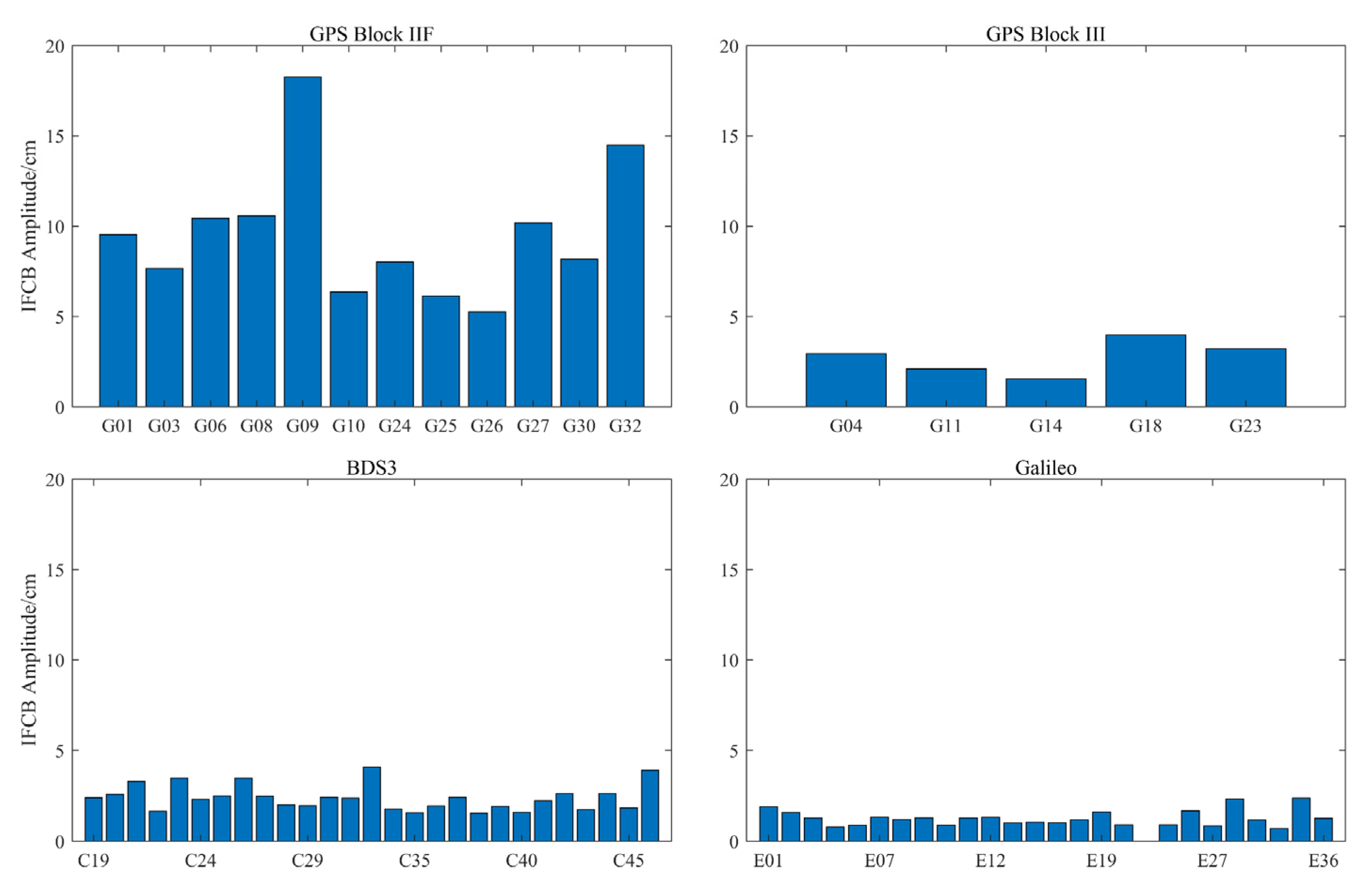
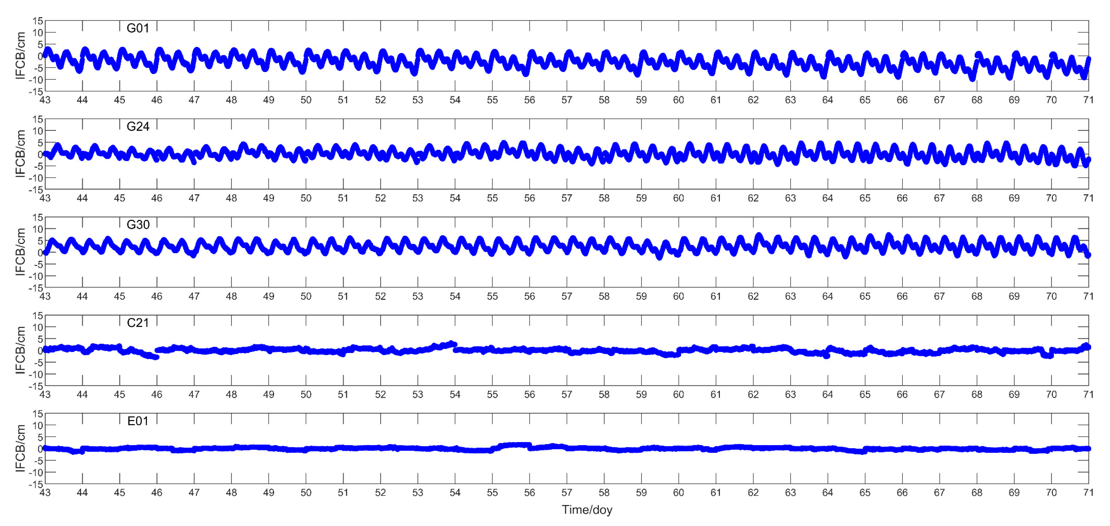
3.2. Time-Varying Feature Analysis of IFCB

3.2.1. Intraday Time-Varying Characteristics Analysis of IFCB

Figure 2 and Figure 3 show the IFCB time series and the IFCB amplitude for each satellite, respectively. It can be seen that the single-day amplitude of GPS Block IIF satellites was large among all, and the amplitude size was between 10 and 20 cm, which is evidently a non-negligible error for PPP. Alternatively, the single-day amplitudes of GPS Block III and BDS-3 satellites were in the range of 1 to 3 cm, and those of the Galileo satellites were below 2 cm. Meanwhile, the standard deviation of IFCB for Block III satellites of the BDS-3, Galileo, and GPS was about 1.5 mm for a single epoch, which was almost unaffected by the IFCB. Therefore, it was necessary to focus on the variation in IFCB of only GPS Block IIF satellites, and analyze the corresponding impact of IFCB on multi-frequency positioning in terms of both positioning performance and residuals; see Section 3.3 and Section 3.4. Since IFCB is considered as a temperature-dependent inter-frequency hardware bias, the different IFCB characteristics of the GPS, BDS-3, and Galileo may be caused by the different designs and payloads of the satellites. However, the IFCBs for GPS Block III and Block IIF satellites express different characteristics and require more information from inside and outside the GPS satellites, for their comprehensive analysis and determination.

3.2.2. Inter-Day Variation Characteristics of IFCB

Figure 4 shows the IFCB time series plot for DOY 43 to 71 in 2022. The IFCB of the GPS Block IIF satellite varied between −15 cm and 15 cm, and exhibited a clear repetitive feature. Meanwhile, the IFCB of Galileo satellites still exhibited relatively small magnitudes, and the large errors in the IFCB of the BDS-3 in some periods were caused by the small number of observable BDS-3 B2a frequency stations present, which indicates that although the IFCB can maintain a good stability and periodicity in most cases, there still exist serious errors in some periods that need further improvement. Montenbruck and Li et al. [13,25,26] found that the IFCB of the GPS Block IIF satellite had 12 and 6 h periods, where the 12 h period is due to the satellite receiving the same amount of sunlight and the 6 h period is due to the satellite having the same amount of heat at two orbital positions around 6 h. Since IFCB has a 6 h and 12 h periodicity expression, it can be further expressed that the IFCB exhibits a 24 h periodicity, and Figure 4 also shows a characteristic single-day periodicity of IFCB. The single-day periodicity of IFCB further assisted in the analysis of the short-term stability of IFCB provided in Section 3.5.

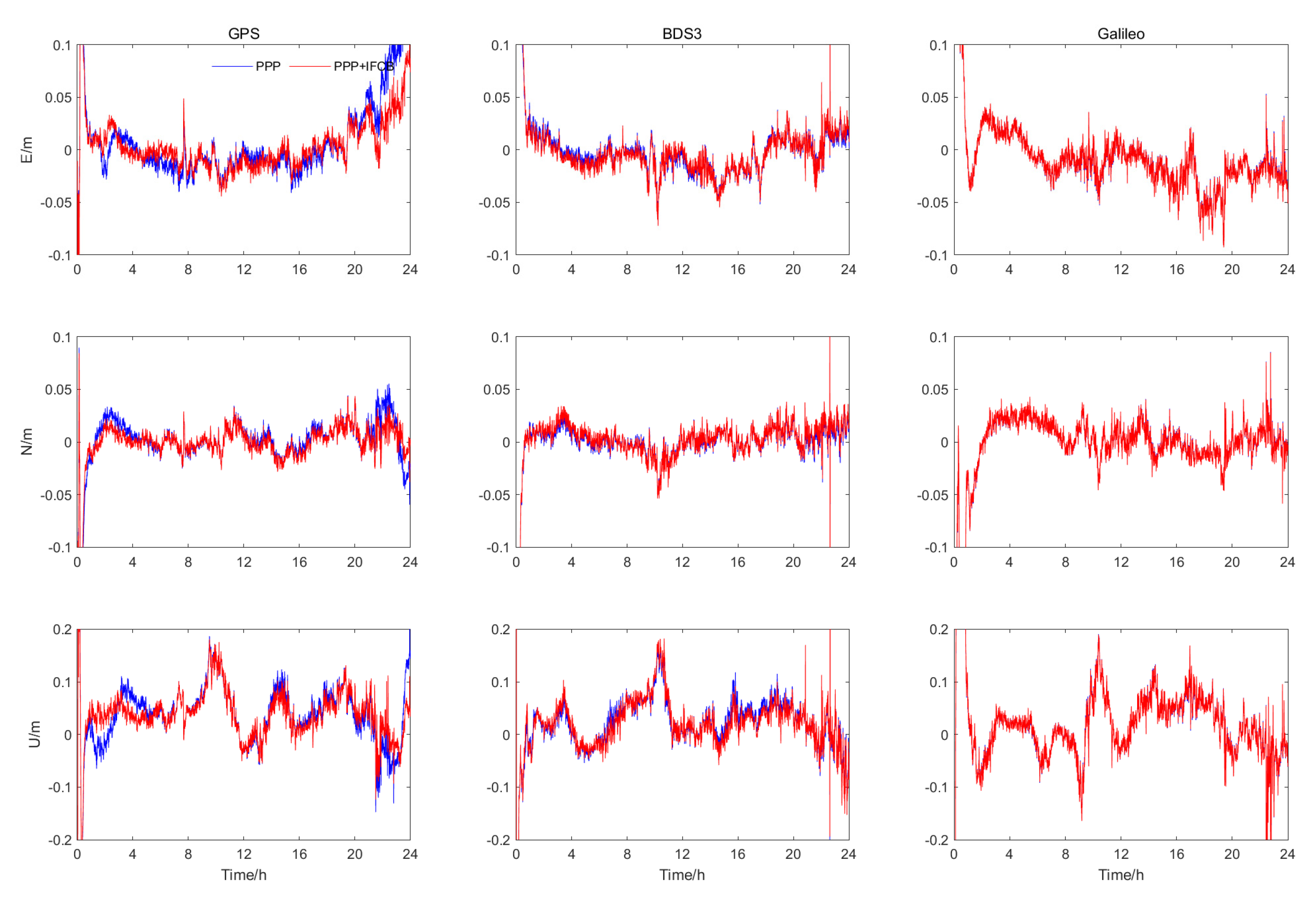
3.3. Triple-Frequency PPP Positioning Performance Analysis

3.3.1. Static Mode

First, the static results of the ASCG station for 2022 DOY 65, from 00:00 UTC to 4:00 UTC, were compared for 1 of the 21 stations. The static PPP positioning error curves under the two solutions of the GPS, BDS-3, and Galileo are shown in Figure 5. During this period, the number of triple-frequency satellites for the ASCG stations of GPS, BDS-3, and Galileo systems was 4.8, 7.6, and 6.6, respectively, indicating that the triple-frequency satellites were involved in the triple-frequency PPP solution.

From Figure 5, it can be observed that the GPS positioning accuracy for the ASCG station was more stable after correcting the IFCB. Meanwhile, for the BDS-3 and Galileo, the change in single-day positioning accuracy was less than 0.1 mm after the IFCB correction, i.e., the positioning accuracy was basically unchanged, which further verifies that the influence of IFCB on the positioning of the BDS-3 and Galileo can simply be ignored. Furthermore, to further analyze the impact of IFCB on GPS positioning, the static PPP accuracy and convergence time under the two scenarios of the GPS at 21 stations for 7 days were recorded, as shown in

Table 3. Statistics of PPP positioning accuracy and convergence time under 7-day GPS static mode for 21 stations (RMS, unit: cm; convergence time, unit: min).

Static	E	N	U	3D	Convergence Time
PPP	1.56	0.60	1.69	2.38	24.19
PPP + IFCB	0.99	0.48	1.34	1.73	21.64
Improvement	36.89%	19.18%	21.16%	27.39%	10.55%

. Without correcting the IFCB, the E, N, U, and 3D positioning accuracy of the GPS system was 1.56 cm, 0.6 cm, 1.69 cm, and 2.38 cm, respectively. On the other hand, following the IFCB correction, the positioning accuracy of the GPS improved to 0.99 cm, 0.48 cm, 1.34 cm, and 1.73 cm, respectively, among which the 3D positioning accuracy was improved by 27.39%. The convergence times for the GPS with corrected and uncorrected IFCB were 21.64 min and 24.19 min, respectively, illustrating a 10.55% improvement in the convergence time. It can be clearly seen that IFCB had a serious impact on the GPS static positioning, and the multi-frequency PPP performance of the GPS was improved by adding the IFCB.

3.3.2. Imitation Kinetic Mode

Regarding the kinematic mode, the results of the ASCG measurement station for 2022 DOY 65 are compared as an example. The positioning error curves under the two schemes of GPS, BDS-3, and Galileo satellites are plotted in Figure 6. During this period, the number of triple-frequency satellites in the GPS, BDS-3, and Galileo systems was 5.2, 7.6, and 6.5, respectively.

As evident from Figure 6, the kinematic and static modes followed a similar pattern, and likewise, the positioning accuracy of the ASCG station GPS was more stable after the IFCB correction, while for the BDS-3 and Galileo, the single-day 3D positioning accuracy was improved from 6.21 cm and 6.30 cm to 6.20 cm and 6.29 cm, respectively, and the change in positioning accuracy was less than 0.1 mm. The statistics related to PPP positioning accuracy and convergence time in the kinematic mode under the two solutions of the GPS at 21 stations for 7 days are provided in

Table 4. Statistics of PPP positioning accuracy and convergence time under 7-day GPS kinematic mode for 21 stations (RMS, unit: cm; convergence time, unit: min).

Kinematic	E	N	U	3D	Convergence Time
PPP	2.59	1.77	4.81	5.74	46.72
PPP + IFCB	2.00	1.43	4.06	4.75	39.61
Promote	22.86%	19.45%	15.53%	17.34%	15.22%

. Without correcting the IFCB, the E, N, U, and 3D positioning accuracy of the GPS was 2.59 cm, 1.77 cm, 4.81 cm, and 5.74 cm, respectively, whereas after the IFCB correction, the GPS positioning accuracy was enhanced to 2 cm, 1.43 cm, 4.06 cm, and 4.75 cm, respectively, where the 3D positioning accuracy was improved by 17.34%. Furthermore, the convergence times for the GPS with corrected and uncorrected IFCB were 21.64 min and 24.19 min, respectively, indicating a 15.22% improvement. Similar to the static mode, the impact of IFCB on the multi-frequency precise point positioning in the GPS kinematic mode was also significant, and the multi-frequency precise point positioning performance of the GPS was further improved by the addition of IFCB.

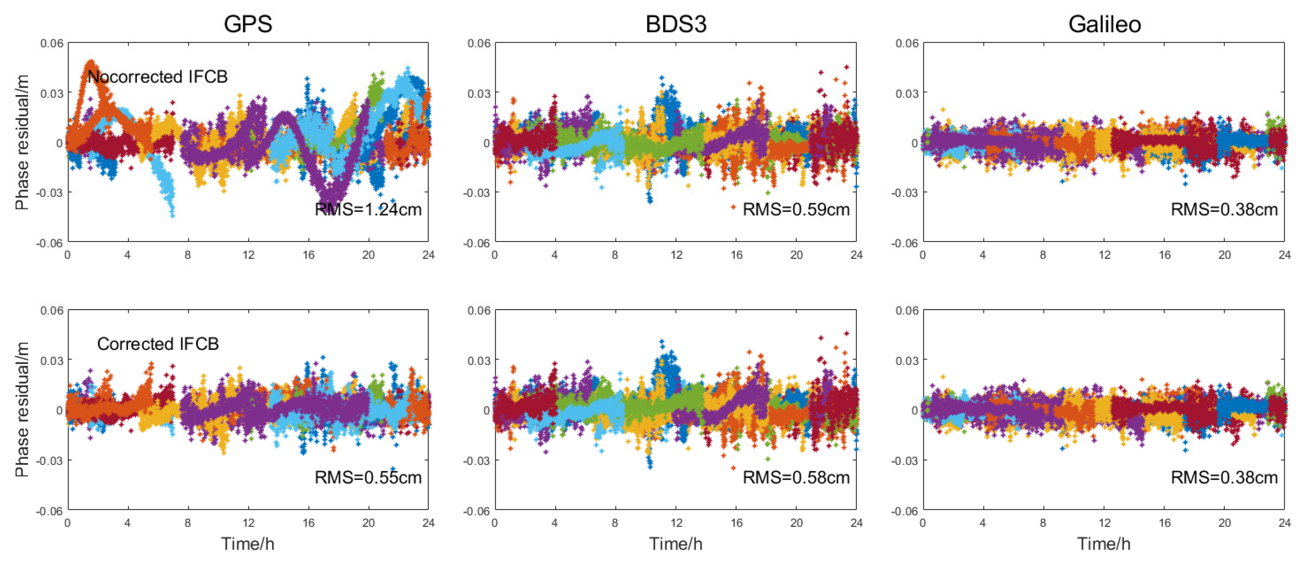
3.4. Model Deviation and Residual Analysis

In addition to the observation noise, some non-modeled errors (e.g., IFCB) were reflected in the post-test residuals of the observation equations, and the time series of the post-test residuals of corrected IFCB and uncorrected IFCB third-frequency phases for the ASCG stations of the GPS, BDS-3, and Galileo are presented in Figure 7. As expected, the GPS without the corrected IFCB exhibited a significant systematic bias effect in the L5 phase residuals, while the IFCB-corrected L5 eliminated this bias effect. Contrary to the GPS, for the BDS-3 and Galileo, the residuals did not show any influence of IFCB, further demonstrating that the IFCB can be neglected for the BDS-3 and Galileo. Meanwhile, to further analyze the effect of IFCB on the GPS L5 phase residuals, the root mean square error of the L5 phase residuals of the GPS at 21 stations for 7 days is given in

Table 5. Root mean square error of GPS L5 phase residuals for 21 stations in 7 days (RMS, unit: cm).

Stations	PPP	PPP + IFCB	Promote	Stations	PPP	PPP + IFCB	Promote
ABPO	1.09	0.43	60.05%	BRUX	1.33	0.23	82.74%
ALIC	1.20	0.35	70.97%	BSHM	1.37	0.30	78.46%
ASCG	1.14	0.55	52.07%	DAV1	0.82	0.36	56.46%
CRO1	1.29	0.46	64.79%	DGAR	1.12	0.48	57.16%
CUSV	1.05	0.35	66.12%	MBAR	1.34	0.44	66.81%
FAA1	1.35	0.55	59.49%	MDO1	1.18	0.33	71.57%
FFMJ	1.34	0.22	83.88%	MET3	1.26	0.30	76.27%
KRGG	1.03	0.43	58.59%	QAQ1	1.13	0.38	66.67%
MAYG	1.19	0.55	53.61%	QUIN	1.25	0.35	71.56%
TOW2	1.17	0.42	63.82%	SUTM	1.19	0.51	57.28%
ULAB	0.98	0.53	45.84%

. The standard deviation of the L5 phase residuals of the GPS before and after the IFCB correction was 1.18 cm and 0.41 cm, respectively, with a 65.12% reduction. Accordingly, it was concluded that after correcting the IFCB, the effect of apparent systematic bias in the L5 residuals of the GPS can be eliminated, and thus, the rejection in the positioning solution process due to excessive residuals can be avoided.

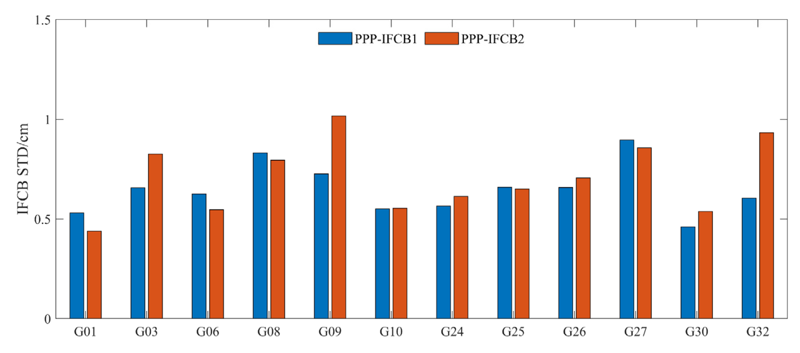
3.5. Short-Term Stability of IFCB

To investigate the short-term stability of IFCB, Figure 8 provides the average STD of IFCB with a one-day delay versus a two-day delay in 2022 for 65 to 71 days. From Figure 8, the average STD of the one-day-delayed and two-day-delayed IFCB was 0.6 and 0.7 cm, respectively. Essentially, the average STD of IFCB of a single satellite did not exceed 1 cm. The statistics for 7-day positioning of 21 stations were recorded using both one-day-delayed and two-day-delayed IFCB, as shown in

Table 6. Statistics of 7-day positioning accuracy and convergence time for 21 stations (RMS, unit: cm; convergence time, unit: min).

Mode		E	N	U	3D	Convergence Time
Static	PPP + IFCB	0.99	0.48	1.34	1.73	21.64
	PPP + IFCB1	0.98	0.48	1.34	1.73	22.16
	PPP + IFCB2	0.99	0.49	1.36	1.76	21.96
Kinematic	PPP + IFCB	2.00	1.43	4.06	4.75	39.61
	PPP + IFCB1	2.01	1.44	4.06	4.76	39.66
	PPP + IFCB2	2.04	1.46	4.09	4.79	39.70

. It can be seen that IFCB products with a one-day delay and a two-day delay could both obtain the same positioning performance as that of the same-day IFCB products to a certain extent, thereby validating the short-term stability of IFCB.

4. Conclusions

IFCB is crucial for high-precision triple-frequency PPP. In this paper, the time-varying characteristics of IFCB for the GPS, BDS-3, and Galileo were analyzed using 117 MGEX station observations, and it was found that the amplitude of GPS Block IIF satellites could reach 10–20 cm, the amplitude of Block III and BDS-3 satellites of the GPS was around 1–3 cm, and the amplitude of Galileo satellites was below 2 cm.

Then, the positioning performance of triple-frequency PPP before and after the IFCB correction was analyzed using the 7-day data from 21 MGEX stations. After the IFCB correction, the positioning performance of BDS-3 and Galileo systems changed negligibly, whereas for the GPS, the 3D positioning accuracies of triple-frequency PPP in static and kinematic modes were improved to 1.73 cm and 4.75 cm, respectively. Compared with the GPS triple-frequency PPP without any IFCB correction, the 3D accuracy post-IFCB-correction improved by 27.39% and 17.34% (static mode and dynamic mode), and the convergence time improved by 10.55% and 15.22% (static mode and dynamic mode), respectively. In addition, the L5 phase post-check residuals of the GPS showed obvious systematic errors. However, the influence of bias could be eliminated by L5 after the IFCB correction. That is to say, the implementation of IFCB estimation can effectively solve the systematic bias problem arising from the multi-frequency positioning results, and realize the unification of traditional clock-difference products and multi-frequency precision positioning.

Since IFCB exhibits obvious periodic characteristics, the short-term stability of IFCB was also investigated in this paper, and the same positioning performance as that of the same day was obtained by using the IFCB products with a one-day delay and a two-day delay.

References

1. Zumberge, J.F.; Heflin, M.B.; Jefferson, D.C.; Watkins, M.M.; Webb, F.H. Precise point positioning for the efficient and robust analysis of GPS data from large networks. J. Geophys. Res. Solid Earth 1997, 102, 5005–5017. [Google Scholar] [CrossRef]
2. Guo, J.; Geng, J. GPS satellite clock determination in case of inter-frequency clock biases for triple-frequency precise point posi-tioning. J. Geod. 2017, 92, 1133–1142. [Google Scholar] [CrossRef]
3. Liu, G.; Zhang, X.; Li, P. Improving the Performance of Galileo Uncombined Precise Point Positioning Ambiguity Resolution Using Triple-Frequency Observations. Remote Sens. 2019, 11, 341. [Google Scholar] [CrossRef]
4. Zhang, X.; Hu, J.; Ren, X. New progress of PPP/PPP-RTK and positioning performance comparison of BDS/GNSS PPP. Acta Geod. Cartogr. Sin. 2020, 49, 1084–1100. [Google Scholar]
5. Su, K.; Jin, S. Analytical performance and validations of the Galileo five-frequency precise point positioning models. Measurement 2021, 172, 108890. [Google Scholar] [CrossRef]
6. Cai, H.; Meng, Y.; Geng, C.; Weiguang, G.; Tianqiao, Z.; Gang, L.; Bo, S.; Jie, X.; Hongyang, L.; Yue, M.; et al. BDS-3 performan ceassessment: PNT, SBAS, PPP, SMC and SAR. Acta Geod. Cartogr. Sin. 2021, 50, 427–435. [Google Scholar]
7. Zhou, F.; Xu, T. Modeling and assessment of GPS/BDS/Galileo treple-frequency precise point positioning. Acta Geod. Cartogr. Sin. 2021, 50, 61–70. [Google Scholar]
8. Zhou, W.; Cai, H.; Chen, G.; Jiao, W.; He, Q.; Yang, Y. Multi-GNSS Combined Orbit and Clock Solutions at iGMAS. Sensors 2022, 22, 457. [Google Scholar] [CrossRef]
9. Yang, X.; Gu, S.; Gong, X.; Song, W.; Lou, Y.; Liu, J. Regional BDS satellite clock estimation with triple-frequency ambiguity resolution based on un-differenced observation. GPS Solut. 2019, 23, 33. [Google Scholar] [CrossRef]
10. Montenbruck, O.; Steigenberger, P.; Prange, L.; Deng, Z.; Zhao, Q.; Perosanz, F.; Romerof, I.; Nollg, C.; Stürzeh, A.; Weber, G.; et al. The Multi-GNSS Experiment (MGEX) of the International GNSS Service (IGS)—Achievements, prospects and challenges. Adv. Space Res. 2017, 59, 1671–1697. [Google Scholar] [CrossRef]
11. Li, B.; Shen, Y.; Zhang, X. Three frequency GNSS navigation prospect demonstrated with semi-simulated data. Adv. Space Res. 2013, 51, 1175–1185. [Google Scholar] [CrossRef]
12. Montenbruck, O.; Hauschild, A.; Steigenberger, P.; Langley, R. Three’s the Challenge: A Close Look at GPS SVN62 Triple-frequency Signal Combinations Finds Carrier-phase Variations on the New L5. GPS World 2010, 21, 8–19. [Google Scholar]
13. Montenbruck, O.; Hugentobler, U.; Dach, R.; Steigenberger, P.; Hauschild, A. Apparent clock variations of the Block IIF-1 (SVN62) GPS satellite. GPS Solut. 2012, 16, 303–313. [Google Scholar] [CrossRef]
14. Pan, L.; Zhang, X.; Li, X.; Liu, J.; Li, X. Characteristics of inter-frequency clock bias for Block IIF satellites and its effect on triple-frequency GPS precise point positioning. GPS Solut. 2017, 21, 811–822. [Google Scholar] [CrossRef]
15. Li, P.; Jiang, X.; Zhang, X.; Ge, M.; Schuh, H. GPS + Galileo + BeiDou precise point positioning with triple-frequency ambiguity resolution. GPS Solut. 2020, 24, 78. [Google Scholar] [CrossRef]
16. Fan, L.; Shi, C.; Li, M.; Wang, C.; Zheng, F.; Jing, G.; Zhang, J. GPS satellite inter-frequency clock bias estimation using triple-frequency raw observations. J. Geod. 2019, 93, 2465–2479. [Google Scholar] [CrossRef]
17. Zhao, Q.; Wang, G.; Liu, Z.; Hu, Z.; Dai, Z.; Liu, J. Analysis of BeiDou Satellite Measurements with Code Multipath and Geometry-Free Iono-sphere-Free Combinations. Sensors 2016, 16, 123. [Google Scholar] [CrossRef] [PubMed]
18. Montenbruck, O.; Hauschild, A.; Steigenberger, P.; Hugentobler, U.; Teunissen, P.; Nakamura, S. Initial assessment of the COMPASS/BeiDou-2 regional navigation satellite system. GPS Solut. 2013, 17, 211–222. [Google Scholar] [CrossRef]
19. Steigenberger, P.; Hauschild, A.; Montenbruck, O.; Rodriguez-Solano, C.; Hugentobler, U. Orbit and Clock Determination of QZS-1 Based on the CONGO Network. Navig. J. Inst. Navig. 2013, 60, 31–40. [Google Scholar] [CrossRef]
20. Zhao, L.; Ye, S.; Song, J. Handling the satellite inter-frequency biases in triple-frequency observations. Adv. Space Res. 2017, 59, 2048–2057. [Google Scholar] [CrossRef]
21. Su, K.; Jin, S.; Jiao, G. GNSS carrier phase time-variant observable-specific signal bias (OSB) handling: An absolute bias perspective in multi-frequency PPP. GPS Solut. 2022, 26, 71. [Google Scholar] [CrossRef]
22. Gong, X.; Gu, S.; Lou, Y.; Zheng, F.; Yang, X.; Wang, Z.; Liu, J. Research on empirical correction models of GPS Block IIF and BDS satellite inter-frequency clock bias. J. Geod. 2020, 94, 36. [Google Scholar] [CrossRef]
23. Li, H.; Li, B.; Xiao, G.; Wang, J.; Xu, T. Improved method for estimating the inter-frequency satellite clock bias of triple-frequency GPS. GPS Solut. 2016, 20, 751–760. [Google Scholar] [CrossRef]
24. Zhang, F.; Chai, H.; Li, L.; Xiao, G.; Du, Z. Estimation and analysis of GPS inter-fequency clock biases from long-term triple-frequency ob-servations. GPS Solut. 2021, 25, 126. [Google Scholar] [CrossRef]
25. Li, P.; Zhang, X.; Ge, M.; Schuh, H. Three-frequency BDS precise point positioning ambiguity resolution based on raw observables. J. Geod. 2018, 92, 1357–1369. [Google Scholar] [CrossRef]
26. Li, H.; Zhou, X.; Wu, B. Fast estimation and analysis of the inter-frequency clock bias for Block IIF satellites. GPS Solut. 2013, 17, 347–355. [Google Scholar] [CrossRef]
Figure 1. MGEX stations used in the experiment. The blue dots represent the stations used to estimate IFCB, and the red dots represent the stations used for PPP validation.
Remotesensing 14 03991 g001
Figure 2. IFCB time series plot for GPS, BDS-3, and Galileo, where each color represents a satellite (DOY 65, 2022).
Remotesensing 14 03991 g002
Figure 3. IFCB amplitudes of GPS, BDS-3, and Galileo satellites (DOY 65, 2022).
Remotesensing 14 03991 g003
Figure 4. IFCB time series plot consisting of G01, G24, G30, C21, and E01 (DOY 43–71, 2022).
Remotesensing 14 03991 g004
Figure 5. ASCG station static mode PPP positioning error curve (DOY 65, 2022; UTC: 00:00 to 4:00).
Remotesensing 14 03991 g005
Figure 6. ASCG station kinematic mode PPP positioning error curve (DOY 65, 2022; UTC: 00:00 to 24:00).
Remotesensing 14 03991 g006
Figure 7. Post-check residual time series of GPS, BDS-3, and Galileo (corrected and uncorrected IFCB) third-frequency phase for ASCG stations (DOY 65, 2022).
Remotesensing 14 03991 g007
Figure 8. IFCB-STD statistics; blue is the STD of the difference between one-day delay and same day, and red is the STD of two-day delay and same day (DOY 65–71, 2022).
Remotesensing 14 03991 g008