
Application of a PLS-Augmented ANN Model for Retrieving Chlorophyll-a from Hyperspectral Data in Case 2 Waters of the Western Basin of Lake Erie

1
Department of Geology and Environmental Geosciences, College of Charleston, University of Charleston, Charleston, SC 29424, USA
2
Naval Research Laboratory, Washington, DC 20375, USA
*
Author to whom correspondence should be addressed.
Remote Sens. 2022, 14(15), 3729; https://doi.org/10.3390/rs14153729
Submission received: 28 June 2022
/
Revised: 30 July 2022
/
Accepted: 1 August 2022
/
Published: 3 August 2022
(This article belongs to the Special Issue Remote Sensing for Water Resources and Environmental Management)
Abstract
:We present results that demonstrate the utility of machine learning techniques that are based on partial least squares (PLS) and artificial neural networks (ANNs) for estimating low-moderate chlorophyll-a (chl-a) concentrations in the western basin of Lake Erie (WBLE). Previous ocean color studies have resulted in a large number of algorithms that are based on spectral indices to estimate water quality parameters (WQPs) such as chl-a concentration from remote sensing reflectance. However, these spectral index algorithms are based on reflectance features at specific wavelengths and do not take advantage of the wealth of spectral information that is contained in hyperspectral data, and are often not easily adaptable to waters with conditions that are different from those in the datasets that were used to originally calibrate the indices. Recently, there have been efforts to use machine learning techniques that are based on ANNs and PLS regression to exploit the spectral richness contained in hyperspectral data and retrieve WQPs. In this study, we have combined an ANN model with output from PLS regression to retrieve chl-a concentration from hyperspectral data in the WBLE. We compared the results from the PLS-ANN method to those that were obtained from a band-ratio algorithm that is based on reflectances in the blue and green spectral regions, a band ratio algorithm that is based on reflectances in the red and near-infrared (NIR) spectral regions, and a PLS-only approach. For a dataset that was collected in 2012, with chl-a concentrations ranging from 0.48 to 21.2 µg/L, the PLS-ANN method yielded a root mean square error (RMSE) of 1.22 µg/L, whereas the blue-green ratio algorithm yielded an RMSE of 1.75 µg/L, the NIR-red ratio algorithm yielded an RMSE of 1.95 µg/L, and the PLS-only approach yielded an RMSE of 1.95 µg/L. The PLS-ANN method takes advantage of the PLS regression to identify specific wavelengths that contain most information about the variation in chl-a concentration, minimize spectral collinearity and redundancy in the data, and simplify the neural network’s input structure. The better performance of the PLS-ANN method can also be attributed to the neural network’s ability to account for nonlinearity in the relationship between chl-a concentration and spectral reflectance. The results indicate that the PLS-ANN method can be reliably used to estimate and monitor low-moderate chl-a concentrations in optically complex waters.
1. Introduction
The spectral response of water in the visible-near-infrared (VNIR) range contains information on the composition of optically significant constituents in water and forms the basis for retrieving water quality parameters (WQPs) such as chlorophyll-a (chl-a) concentration from satellite data [1]. Historically, methods employed to quantitatively retrieve WQPs from remote sensing signals have included semi-empirical regression techniques that are based on ratios of or differences between reflectances at two or three spectral regions [2,3,4,5] and spectral inversion techniques that are based on the radiative transfer model e.g., [6,7]. In optically complex Case 2 waters [8] such as the Western Basin of Lake Erie (WBLE) [9], where the spectral signature is a function of multiple, non-covarying WQPs, retrieving estimates of various WQPs using reflectance at only a few select bands is challenging [10]. Approaches that are based on spectral feature selection and full spectral optimization to determine an optimal set of solutions for retrieving numerous WQPs from individual satellite-measured reflectance spectra have been attempted but found to be computationally too expensive and too time-consuming for operational implementation, especially when they are implemented on a per-pixel basis on local processors [11,12]. With the introduction of Application Programming Interfaces (APIs) that are run on cloud computing infrastructure such as the Google Earth Engine, the computational burden has become less critical of an issue, and there is renewed interest in using full spectral optimization as an operational tool to retrieve WQPs from hyperspectral data e.g., [13]. Several spaceborne hyperspectral sensors have been launched recently or are scheduled to be launched in the near future, resulting in an abundance of global hyperspectral data for the next several years, ready to be exploited for environmental monitoring and resource management purposes. The sensors include the recently launched Italian mission PRecursore IperSpettrale della Missione Applicativa (PRISMA), the recently launched German mission Environmental Mapping and Analysis Program (EnMAP), and NASA’s future hyperspectral missions, the Plankton, Aerosol, Cloud, ocean Ecosystem (PACE) mission and the Surface Biology and Geology (SBG) mission, both of which are currently under development.
With the availability of large volumes of high dimensional remote sensing data and enhanced computational efficiency, linear methods such as the partial least squares (PLS) regression and machine learning techniques such as the artificial neural network (ANN), which is well suited for modeling non-linear relationships, are increasingly being applied in many remote sensing studies. In 1999, Schiller and Doerffer [14] developed a neural network (NN), which was later applied to data from the multispectral MEdium Resolution Imaging Spectrometer (MERIS) to retrieve concentrations of chl-a and suspended particulate matter (SPM) [15]. Several other NN-based approaches have also been developed to retrieve WQPs, especially chl-a concentration, from satellite data (e.g., [16,17,18,19,20,21]), with varying levels of success. In general, NN-based approaches tend to yield accurate estimates when they are applied to data from waters with biophysical conditions within the range of parameters that are used to train the NN model and fail when they are applied to conditions outside the training data range. This is a limitation, especially for multispectral NN-based algorithms that are based on modeled relationships between WQPs and reflectance at a few specific wavelengths. Hyperspectral data offer the ability to capture minor spectral variations in optical properties of water and its constituents and are well suited for optically complex waters. However, hyperspectral images contain large volumes of data that are inherently collinear, with often significant correlation amongst adjacent spectral channels. The large volume of the data and high correlation amongst data variables can introduce complexity to the neural network and can lead to overfitting of the model [21,22], thereby yielding inaccurate estimates. It is, therefore, necessary to reduce dimensionality and multicollinearity in hyperspectral data before applying NN-based algorithms. Data dimensionality and multicollinearity can be reduced by using methods such as the PLS, resulting in a low-dimensional dataset with a simplified structure, consisting of variables that are most significant for explaining variations in the dataset. PLS reduces the spectrally rich hyperspectral dataset to an optimal, low-dimensional set of variables that are most sensitive to parameters of interest to be retrieved. Once the redundancy and multicollinearity in the data are removed or minimized, ANNs are well suited to account for nonlinearity in the dataset and retrieve the parameter of interest. Optimized neural network algorithms that are based on feature dimension reduction have been successfully used for many applications [23].
Because of the complementary advantages of PLS and ANN, we combined both methods in a two-step process to estimate chl-a concentration in optically complex waters of the western basin of Lake Erie (WBLE) using hyperspectral data. A similar approach has been previously tested by Song et al. [24], who applied a PLS-ANN approach to datasets from several inland water bodies in Indiana, USA, and China for retrieving chl-a concentration and reported that the PLS-ANN approach yielded accurate results, marginally outperforming a three-band model that was based on reflectances in the red and near-infrared (NIR) spectral regions. The dataset that was used by Song et al. [24] encompassed a very wide range of chl-a concentrations, ranging over two orders of magnitude. While the overall accuracy reported by Song et al. [24] for the PLS-ANN algorithm is high for the entire range of chl-a concentrations, one may wonder whether similar accuracies may be obtained if the algorithm is applied to data from optically complex waters with a narrower range of low-moderate chl-a concentrations. Accurate retrieval of low-moderate chl-a concentrations (~5–15 ) in optically complex, Case 2 waters [8] is often problematic [25,26,27,28,29] because it is at the high end of sensitivity for algorithms that rely on chl-a-specific features in the blue and green spectral regions and at the low end of sensitivity for algorithms that rely on chl-a-specific features in the red and NIR spectral regions. Moreover, at low-moderate chl-a concentrations, chl-a-specific spectral features at wavelengths of interest are affected, and in some cases overwhelmed, by contributions from other optically significant constituents such as SPM and colored dissolved organic matter (CDOM). The objective of this study is to test the suitability of the PLS-ANN approach for retrieving low-moderate chl-a concentrations, using as a case study the WBLE, which is an optically complex water body [9] with significant concentrations of SPM and CDOM, which do not co–vary with chl-a concentration. We focused on data that were collected in late spring and early summer, before chl-a concentrations attain peak values. First, we used the PLS framework to assess the relationship between hyperspectral reflectance measurements and chl-a concentrations and identify the spectral channels of importance that contribute significantly to explaining variations in chl-a concentration. We also used PLS to identify spectral channels that are highly correlated to each other and used the information to reduce dimensionality and multicollinearity in the hyperspectral dataset. Second, we used information from the PLS output in an ANN framework to model the nonlinear relationship between hyperspectral reflectance and chl-a concentrations, determine the relative importance and predictive value of the input wavelengths, and estimate chl-a concentration. We have also provided estimates of chl-a concentration retrieved through the PLS method alone and through well-established semi-empirical algorithms that are based on the blue-green and NIR-red reflectance ratios for the sake of comparison with PLS-ANN retrievals.
2. Data and Methods
2.1. Data
The data consisted of reflectance and chl-a concentrations that were collected from 18 stations in the WBLE (Figure 1) in June and July of 2012 using the research vessel Gibraltar III.
2.1.1. Reflectance Measurements
Hyperspectral data were collected at each station using a GER 1500 Visible and Near-Infrared (VIS-NIR) spectroradiometer at continuous wavelengths within the spectral range 350–1080 nm at 1.5 nm spectral intervals and 3.2 nm spectral resolution. Upwelling radiance, and downwelling irradiance, were collected simultaneously. To minimize adjacency effects from the vessel, the measurements were taken from the sun-lit side of the vessel using an optical fiber that was attached to an extendable pole, with the tip of the optical fiber placed a few centimeters below the water surface and pointed towards nadir. In order to minimize the effect of uncertainties due to noise, six spectra were taken and averaged for each station. Each average spectrum was then spectrally averaged at 10 nm intervals between 400 and 750 nm, resulting in 36 spectral channels of data for each spectrum. A white Spectralon® reflectance standard was used to calibrate the GER 1500 spectra. The remote sensing reflectance (Rrs) was calculated by normalizing the upwelling radiance, by the downwelling irradiance, as follows [30]:
where and are the upwelling radiance from and the downwelling irradiance incident on the Spectralon® reflectance standard, respectively, is the known irradiance reflectance of the Spectralon® reflectance standard, is used to transform the irradiance reflectance into remote sensing reflectance, is the water-to-air transmittance (), is the refractive index of water relative to air (n = 1.34 at 20 °C), and is the spectral immersion factor, which accounts for the radiance transfer between water and air [31,32].
Figure 2 shows hyperspectral data that were collected from the WBLE. The spectral signatures are characteristic of productive waters with absorption and scattering features across various spectral regions [30,33,34]. The features are indicative of the effects of optically significant in-water constituents, such as absorption and scattering of phytoplankton and other associated WQPs. Absorption minima near the green (560 nm) and NIR (710 nm) spectral regions and maxima near 440, 620, and 680 nm are clearly apparent in the data; these features indicate the presence of phytoplankton biomass [35,36,37]. The NIR reflectance peaks are much higher for chl-a concentrations > 1.5 . The absorption minima near 560 nm and the maxima near 680 nm are more distinct for samples from stations that are closer to stream and river inlets, such as in the Sandusky Bay, compared to those further offshore in the open waters of the WBLE (Figure 1).
2.1.2. Chl-a Measurements
At each of the 18 stations, water samples were collected at 0.5 m depth, filtered using glass fiber filters (GF/F), and temporarily stored in a freezer at −20 °C for subsequent analysis in the laboratory. Chl-a was extracted from the samples and quantified following the U.S. Environmental Protection Agency’s (EPA) 445 protocol [38]. The average in situ chl-a concentration for the whole dataset was 4.83 . The concentration tended to increase throughout the sampling period. The concentrations across the basin varied between 0.48 and 21.2 , with higher concentrations recorded at stations located in the Sandusky Bay (Figure 1). The standard deviation of the chl-a concentrations was 4 (Figure 3). The high standard deviation is attributed to the relatively higher seasonal algal density in the Sandusky Bay. During late spring and early summer, river discharges are high, and significant amounts of terrestrial matter, including nutrients, are transported into the bay. This increases the combined concentrations of allochthonous and autochthonous phytoplankton and, consequently, leads to higher chl-a concentrations in the bay (Stations 17, 19 and 20—see Figure 1), which results in significant differences in chl-a concentration between the waters in the Sandusky Bay and the central WBLE. By late summer, the river discharge decreases and the waters between the two sub-basins undergo mixing, resulting in a decrease in the overall variability of chl-a concentration in the WBLE [3].
2.2. Methods
The data were analyzed to retrieve the chl-a concentrations using partial least squares, artificial neural network, and two well-established semi-empirical algorithms—a blue-green algorithm and an NIR-red algorithm.
2.2.1. Partial Least Squares (PLS)
PLS is a feature-reduction approach that has the ability to analyze data with a low signal-to-noise ratio and numerous, strongly collinear variables [39]. It projects relationships between two sets of matrices containing dependent and independent variables onto a latent space, extracting several principal independent factors while capturing most of the variance in the original data [40,41,42].
Suppose there are n observations of K feature variables, and m dependent variables, . In an aquatic remote sensing context, K represents the number of spectral channels in the reflectance dataset and m represents the number of WQPs that are being retrieved from the reflectance measurements. As with Principal Component Analysis (PCA), the data are mean-centered and scaled to ensure zero mean and unit variance. The preprocessed data matrix X is expressed as:
Here, is the score matrix, which contains the iterative projections of the observed data onto successive orthogonal axes or components of maximum variation (akin to the principal components in PCA) and has the dimension n × A, where n is the number of observations in the dataset and A is the number of components; is the load matrix, which consists of unit vectors, each describing the direction of the respective component, and has the dimension K × A; is the residual error matrix, which is an n × K matrix consisting of the perpendicular distance between each observation data point and the hyperplane, which encompasses all components. For a given component, i, the matrix multiplication can be expressed as the sum product of the score vector (the ith column of the score matrix T) and the load vector (the ith column of the loading matrix P). For a system with A principal components, Equation (2) can be rewritten as:
Similarly, matrix Y is decomposed into:
Y = UQT + F
Here, U is the score matrix, Q is the loading matrix, and F is the residual error matrix. For a given component, i, the matrix multiplication UQT can be expressed as the sum product of the score vector ui (the ith column of the score matrix U) and the loading vector qi (the ith column of the loading matrix Q); Equation (4) can be rewritten as:
PLS differs from PCA in that the score matrices are determined for both dependent and independent variables. Moreover, the score matrix T is determined based on not only X but also Y. For a given component , each of the K columns in is regressed against an initial estimate of to determine a weight vector, , which is normalized to unit length and regressed against every row in to determine the score vector Similarly, every column in (each representing the m WQPs to be retrieved) is regressed against to determine a weight vector for the Y data space, , which is regressed against every row in to determine the score vector . The process continues iteratively until changes negligibly. At convergence, and together define the component and are stored in the respective matrices W, T, Q, and U. One of the salient features of the PLS is that the score matrices T and U not only maximally explain the variance in the X and Y data space but they also maximize the covariance, and hence the correlation, between ti and ui. Thus, they represent not only the best explanations of variance in the X and Y data space but also the best explanation of the relationship between X and Y. The model predictions of the X and Y matrices at the ith component are determined as follows:
where is the loading vector that is determined by regressing the columns of against , and:
The data matrices are deflated and new matrices for the next component are determined as and . The process continues until successive components do not explain new variability. When used for predicting the dependent variables, the relationship between the score matrix T and the data matrix X is exploited to predict Y. Given that the weight vectors for successive components are calculated based on deflated X matrices and not the original data matrix, W cannot be directly used to define the relationship between T and X. The loading matrix, P, and the weight matrix with deflation, W, can be combined as , which relates T and X as:
The weight matrix R is informative as it indicates the importance of the dependent variables in X space for explaining the variation in Y. In the aquatic remote sensing context, the matrix R helps to identify spectral channels of importance for estimating the WQPs of interest in Y. Spectral channels containing similar information will have similar weights. Thus, R also provides a means of minimizing data redundancy.
Following Equation (7), Y can be calculated as:
Using Equation (8) in Equation (9), we get:
is the regression coefficient of the PLS model.
PLS accounts for spectral correlation amongst the various spectral channels, assigns weights to the spectral channels depending on their predictive capability, and enhances the potential discrimination of retrieved constituents. PLS does not need to use all of the input hyperspectral channels to establish maximum correlation with WQPs. It only needs information from select spectral channels. As such, it provides a convenient way to minimize multicollinearity and reduce dimensionality in the dataset.
2.2.2. Artificial Neural Network (ANN)
ANNs provide a powerful means to get insight into and uncover underlying nonlinear relationships and structures that are existing in datasets [43]. ANN imitates the biological neural network learning process and possesses powerful functions for dealing with nonlinear processes with complex underlying structures. The model is formed by artificial neurons on multiple layers including input/output that emulate biological neurons and the synaptic connections.
The feed-forward back-propagation multi-layer perceptron (MLP) is the most frequently used ANN in remote sensing applications [44]. The basic structure is comprised of three distinctive layers: (i) the input layer, where the remote sensing reflectance data are introduced into the model, represented by the array ; (ii) the hidden layer, where the activation function is applied to after multiplying it by the corresponding synaptic weight vector, , for data transformation; and (iii) the output layer, where the results, , of the ANN are produced [45,46]. The ANN is trained through a backpropagation algorithm to minimize the error between the predicted and expected outputs. The error is redistributed by recomputing for the previous neuron layers from back to front [47]. The backward iteration processes and the step size that is taken to update is controlled by the ANN learning rate, expressed as:
2.2.3. Semi-Empirical Algorithms
For the sake of comparison with the PLS and PLS-ANN methods, we retrieved chl-a concentrations using two well-established semi-empirical algorithms, one that is based on reflectance in the blue and green spectral regions and the other based on reflectance in the red and NIR regions.
Blue-Green Chl-a Algorithm
Recently, O’Reilly and Werdell [4] used an extensive collection of global datasets to re-parameterize the blue-green algorithm that was originally developed decades ago by O’Reilly et al. [48]. The blue-green chl-a algorithm is a fourth-degree polynomial equation of the form:
where, , and , , , , and are polynomial coefficients obtained by regressing the maximum blue-green ratio values against measured chl-a concentrations. O’Reilly et al. [4] developed regression coefficients for 25 spaceborne sensors, taking into consideration minor variations across the sensors in the wavelength locations of respective spectral channels in the blue and green regions.
Considering the wavelengths of the GER 1500 spectrometer, we used a 4th order polynomial function [4] for a wavelength combination that was closest to spectral channels centered at 440 nm, 490 nm, and 510 nm in the numerator and 560 nm in the denominator. The specific optimized algorithm was:
where: .
NIR-Red Chl-a Algorithm
The two-band NIR-red model that is based on the chl-a absorption feature in the red spectral region and the reflectance peak in the NIR region due to the combined effect of decreasing absorption of light by chl-a and increasing absorption by water [49,50] has yielded accurate retrievals of chl-a concentrations in various inland and coastal waters around the world when applied to in situ, airborne, and spaceborne remote sensing data.
Based on the wavelength locations of the red and NIR spectral channels of the GER 1500 spectrometer, an optimized two-band NIR-red algorithm, with the coefficients re-parameterized based on in situ measurements of chl-a concentration from the WBLE, was formalized as follows:
It must be noted that the wavelengths at the red and NIR spectral channels of the GER 1500 spectrometer used in this study, namely 670 and 710 nm, are slightly different from the original red and NIR wavelengths that were used in the development of the two-band NIR-red model [51], namely 665 and 708 nm. This could have an impact on the algorithm performance, although we expect the impact of the wavelength difference to be negligible.
3. Results and Discussions
Chl-a concentrations were estimated using the PLS method, PLS-ANN method, the blue-green algorithm, and the two-band NIR-red algorithm. As the dataset was rather small, it was not split into separate calibration and validation datasets. Instead, each of the algorithms was applied to the entire dataset and the retrievals were assessed by comparing them to in situ measurements. The goal of this study is not to develop universally applicable PLS-ANN algorithms but to rather test the suitability of the approach for a small dataset with low-moderate chl-a concentrations.
3.1. Error Metrics
The retrieved chl-a concentrations were evaluated based on the correlation coefficient (), root mean square error (RMSE), and three additional error metrics that were recommended by Seegers et al. [52], namely, mean absolute error (MAE), bias, and ‘percent wins’. It must be noted that is limited in its utility as a validation metric because a high does not necessarily mean high accuracy if there is significant bias in the estimates. Nevertheless, it can be used as a measure of consistency in the algorithm’s behavior across the range of measurements. The MAE and bias are expressed as multiplicative metrics that were calculated by first log-transforming the retrievals to determine the residuals as log-transformed measures and back-transforming them. This approach is well suited for quantities such as chl-a concentration for which the error varies proportionally with the magnitude of the quantity [52]. The calculated MAE and bias are to be interpreted as multiplicative measures. For example, an MAE of 1.25 would indicate a relative measurement error of 25% and a bias of 1.3 would mean that the estimate is on average 30% more than the observed value, with bias values that are less than unity indicative of negative bias. The RMSE, MAE, and bias are expressed as follows:
where and are the estimated and measured values, respectively, and n is the number of observations. It must be noted that while the MAE reported here is a unitless measure that is based on log-transformed values, the RMSE is in physical units of chl-a concentration determined based on untransformed values and, as such, the numerical magnitudes of MAE and RMSE cannot be compared against each other.
The ‘percent wins’ was calculated according to the steps that were described by Seegers et al. [52], in which each data point was examined individually, and for each data point, the algorithm that yielded the closest estimate to the observed measurement was declared the ‘winner’. For each algorithm, the ‘percent wins’ is the percentage of data points for which its estimate was the closest in value to the measured value in comparison to estimates from the other algorithms. This is a valuable diagnostic metric that provides additional information on the algorithms’ performance, such as identifying algorithms that yield very accurate estimates for some data points but fail significantly at other data points, which might provide insights on optimal conditions for those algorithms. It also helps to identify algorithms that may not yield the best or the worst estimates but may perform consistently well across all data points in the dataset.
3.2. Estimation of Chl-a Concentration Using the PLS Method
Distributional transformation was applied to the original input data to get the characteristic input variables in matrix (hyperspectral remote sensing data) and output variables in matrix (measured chl-a concentrations). The data were mean-centered and standardized with a distribution of N(0,1). This ensures data normality, eliminates intrinsic numerical influence, overcomes model learning problems, and allows easy data comparison. PLS was then applied to reduce multicollinearity in the dataset and extract the leading components t and u from X and Y, respectively, while maximizing their correlation with each other and projecting the regression of X on the t axis and Y on the u axis. The new components represent relevant information that is present in the reflectance spectra that were used to estimate the chl-a concentration. Similar methods have been previously applied [53,54] for extracting information about spatial and temporal variations in sediment composition. The method works well for optically significant in-water constituents, allowing the extraction of absorption features that are correlated to the presence of chl-a. In many cases, spectral patterns identified by PLS can also be interpreted physically based on known spectral signatures [10,12,55].
The application of the PLS model to the input hyperspectral data, , generated three principal components, , which explained more than 96% (Figure 4) of the optical variance recorded in the data. The three principal components represent latent spectral structures that are obtained by maximizing the covariance between linear combinations of spectral bands and chl-a concentrations in the WBLE. The first component explained about 63% of the observed chl-a variability, and the second and third factors explained 9% and 24% of the chl-a variability, respectively. This suggests that the spectral bands that have relatively higher communality in the PLS components are the most sensitive to chl-a variability. These include bands that are centered at 690, 700, 710, and 720 nm in PLS factor 1 (components); spectral regions near 440, 480, 490, 560, 580, 620, 650, 670, 680, 700, and 710 nm were identified as the most sensitive to chl-a variations in PLS factors 2 and 3 (Figure 4), consistent with previous studies [5,10,55]. The correlation between the retrieved individual principal components, , and chl-a, as shown in Figure 5, indicates the linear relationship of each component to the PLS-based chl-a model. Comparison between the measured chl-a concentrations and estimates from the PLS model yielded an of 0.76, an RMSE of 1.95 , an MAE of 1.41, a bias of 1.16, and a percent-wins measure of 16.28% (Table 1).
3.3. Estimation of Chl-a Concentration Using the PLS-ANN Method
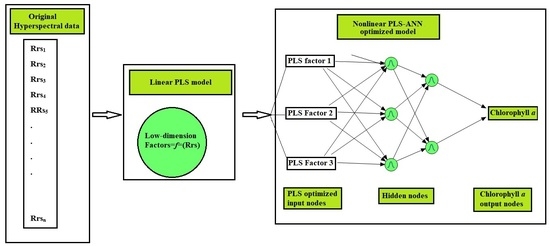
The dimension-reduced output from the PLS process, and , are supplied as input into the ANN as the predictor and response variables, respectively. The network employed in this study is a two-layer perceptron that is based on backpropagation (Figure 6). The first layer has two nodes, and the second layer has three nodes. Each of the two nodes in the first layer is a function of all three nodes in the second layer. All three nodes in the second layer are a function of the reduced-dimension input spectra, . The estimated chl-a concentration (i.e., ) is a function of both nodes in the first layer. The PLS-ANN model was initially trained using a randomly selected training data subset representing 75% of the dataset. The remaining 25% was used to assess the model’s capability to estimate chl-a concentration in the WBLE.
Augmenting the PLS model with an ANN helps model nonlinearities that may exist between the spectral-based PLS factors and chl-a concentration, which the PLS may not necessarily capture. Figure 7 shows the linear and nonlinear components of the relationship between the three PLS factors (PLS X, scores 1–3) and chl-a concentrations on the y axis. The slopes of the relationships are indicative of the extent of variability in chl-a concentration that is captured by each factor, with steeper slopes indicative of higher proportions of the variability captured by the model. In this case, PLS Factor 1 captures significantly more linear and nonlinear components than do PLS Factors 2 and 3. A comparison between the measured chl-a concentrations and PLS-ANN estimates (Figure 8b) yielded an of 0.92, an RMSE of 1.22 , an MAE of 1.31, a bias of 1.1, and a percent-wins measure of 58.14% (Table 1), all of which are better than the corresponding figures from the PLS-only approach.
3.4. Estimation of Chl-a Concentration Using the Blue-Green Algorithm
The blue-green algorithm yielded reasonably accurate estimates of chl-a concentration (Figure 8c). The algorithm performed fairly well at low chl-a concentrations, although the plot of measured vs. estimated concentrations shows some scatter around the 1:1 line. The algorithm underestimated moderate chl-a concentrations, which is consistent with previous observations regarding the limitations of the blue-green algorithm at moderate-to-high chl-a concentrations [50].
The chl-a estimates from the blue-green algorithm had an of 0.61, an RMSE of 1.75 , an MAE of 1.73, a bias of 1.21, and a percent-wins measure of 12.79%.
3.5. Estimation of Chl-a Concentration Using the NIR-Red Algorithm
The two-band NIR-red algorithm also yielded reasonably accurate estimates of chl-a concentration (Figure 8d). Unsurprisingly, the algorithm performed poorer at low chl-a concentrations (<5 ), where the chl-a-specific spectral features are weaker in the red and NIR spectral regions and the effect of uncertainty due to low signal in the NIR region becomes more pronounced. The algorithm performed fairly well at moderate chl-a concentrations, although the estimates were biased low. The chl-a estimates from the two-band NIR-red algorithm had an of 0.56, an RMSE of 1.95 , an MAE of 1.74, a bias of 1.19, and a percent-wins measure of 12.79% (Table 1).
The performance metrics for the algorithms are summarized in Table 1. Among the algorithms, the PLS-ANN algorithm performed the best in estimating the chl-a concentration. This is further confirmed using the regression plots that are presented in Figure 8, with show the hybrid model with the highest value and the least RMSE value.
4. Conclusions
This study shows that the PLS-ANN model, which combines linear (i.e., PLS) and nonlinear modeling (i.e., ANN), can be used to retrieve accurate and reliable estimates of chl-a concentration from hyperspectral data. The PLS-ANN model produced the best result in each of the five error metrics that were used to assess the chl-a estimates, followed by the PLS model and the band ratio algorithms. The results are consistent with those obtained by Song et al. [24], who compared chl-a estimates from the PLS-ANN method with those from the PLS-only and NIR-red band ratio models. As stated earlier, this study differed from that of Song et al. [24] in that we focused on low-moderate chl-a concentrations. One of the challenges with algorithms parameterized using datasets with a very wide range of chl-a concentrations is that the published overall performance metrics of the algorithm may be heavily influenced by values towards the extreme ends of the data range, and one may not be sure if the algorithm will yield the same accuracy when it is applied to a dataset representing a narrower range of conditions. This study demonstrates that the PLS-ANN method works reliably well at low-moderate chl-a concentrations, which is a critical range of transition from mesotrophic to eutrophic waters, which is outside the typical chl-a range for algorithms that are meant for oligotrophic waters and at the low end of the chl-a range for algorithms that are parameterized for eutrophic waters.
One of the unique advantages of the PLS-ANN model is the ability to model both linear and nonlinear components of the relationship between chl-a concentration and hyperspectral reflectance, which is critically important for optically complex, Case 2 waters. The PLS approach helps minimize collinearity in the dataset and reduce the input hyperspectral dataset into fewer components that explain most of the variation in the parameter of interest. In this study, the first three PLS components (factors) altogether explained 96% of the variation in chl-a concentration. By reducing data dimensionality and multicollinearity, the PLS approach helps to minimize potential overfitting problems, which can be a significant concern with hyperspectral data.
As demonstrated in this study, the PLS-ANN model is well-suited to take full advantage of spectral information that is contained in hyperspectral data to retrieve WQPs in optically complex water bodies such as the WBLE. The goal of this study was not to develop a universally applicable PLS-ANN algorithm for estimating chl-a concentration but to test the suitability of the approach for a specific case of low-moderate concentrations. A much larger dataset encompassing a wide range of biophysical conditions is needed for developing algorithms for broader application to multiple water bodies without the need for site-specific calibration. A key consideration in developing such a universal algorithm would be consistency in the spectral channels that are associated with the most significant PLS factors.
As hyperspectral data become increasingly common around the world, tools that are based on approaches such as the PLS-ANN model, which makes effective use of spectrally rich data, will be critical for monitoring environmental changes in optically complex inland, estuarine, and coastal waters.
Author Contributions
Conceptualization: K.A.A.; methodology: K.A.A. and W.J.M.; software: K.A.A.; validation: K.A.A.; formal analysis: K.A.A. and W.J.M.; investigation: K.A.A. and W.J.M.; resources: K.A.A. and W.J.M.; data curation: K.A.A.; writing—original draft preparation: K.A.A.; writing—review and editing: K.A.A. and W.J.M.; visualization: K.A.A.; supervision: K.A.A. and W.J.M.; project administration: K.A.A. and W.J.M.; funding acquisition: K.A.A. and W.J.M. All authors have read and agreed to the published version of the manuscript.
Funding
This research was funded by NASA’s R3 funding, grant number SC-80NSSC20M0148 and basic research funds from the U.S. Naval Research Laboratory.
Acknowledgments
We acknowledge NASA’s EPSCoR program and the U.S. Naval Research Laboratory for funding this research.
Conflicts of Interest
The authors declare no conflict of interest. The funders had no role in the design of the study; in the collection, analyses, or interpretation of data; in the writing of the manuscript; or in the decision to publish the results.
References
- Albert, A.; Mobley, C. An analytical model for subsurface irradiance and remote sensing reflectance in deep and shallow case-2 waters. Opt. Express 2003, 11, 2873–2890. [Google Scholar] [CrossRef]
- Ali, K.A.; Ortiz, J.; Bonini, N.; Shuman, M.; Sydow, C. Application of Aqua MODIS sensor data for estimating chlorophyll a in the turbid Case 2 waters of Lake Erie using bio-optical models. GISci. Remote Sens. 2016, 53, 483–505. [Google Scholar] [CrossRef]
- Ali, K.; Witter, D.; Ortiz, J. Application of empirical and semi-analytical algorithms to MERIS data for estimating chlorophyll a in Case 2 waters of Lake Erie. Environ. Earth Sci. 2014, 71, 4209–4220. [Google Scholar] [CrossRef]
- O’Reilly, J.E.; Werdell, P.J. Chlorophyll algorithms for ocean color sensors—OC4, OC5 & OC6. Remote Sens. Environ. 2019, 229, 32–47. [Google Scholar] [CrossRef]
- Moses, W.J.; Gitelson, A.A.; Berdnikov, S.; Bowles, J.H.; Povazhnyi, V.; Saprygin, V.; Wagner, E.J.; Patterson, K.W. HICO-Based NIR–Red Models for Estimating Chlorophyll-α Concentration in Productive Coastal Waters. IEEE Geosci. Remote Sens. Lett. 2013, 11, 1111–1115. [Google Scholar] [CrossRef]
- Lee, Z. Visible-Infrared Remote Sensing Model and Applications for Ocean Waters; University of South Florida: Tampa, FL, USA, 1994. [Google Scholar]
- Roesler, C.S.; Perry, M.J. In situ phytoplankton absorption, fluorescence emission, and particulate backscattering spectra determined from reflectance. J. Geophys. Res. Ocean. 1995, 100, 13279–13294. [Google Scholar] [CrossRef]
- Morel, A.; Prieur, L. Analysis of variations in ocean color1. Limnol. Oceanogr. 1977, 22, 709–722. [Google Scholar] [CrossRef]
- O’Donnell, D.M.; Effler, S.W.; Strait, C.M.; Leshkevich, G.A. Optical characterizations and pursuit of optical closure for the western basin of Lake Erie through in situ measurements. J. Great Lakes Res. 2010, 36, 736–746. [Google Scholar] [CrossRef]
- Ali, K.A.; Witter, D.L.; Ortiz, J.D. Multivariate approach to estimate colour producing agents in Case 2 waters using first-derivative spectrophotometer data. Geocarto Int. 2013, 29, 102–127. [Google Scholar] [CrossRef]
- Doerffer, R.; Fischer, J. Concentrations of chlorophyll, suspended matter, and gelbstoff in case II waters derived from satellite coastal zone color scanner data with inverse modeling methods. J. Geophys. Res. Earth Surf. 1994, 99, 7457–7466. [Google Scholar] [CrossRef]
- Ryan, K.; Ali, K. Application of a partial least-squares regression model to retrieve chlorophyll-a concentrations in coastal waters using hyper-spectral data. Ocean Sci. J. 2016, 51, 209–221. [Google Scholar] [CrossRef]
- Van Nguyen, M.; Lin, C.-H.; Chu, H.-J.; Jaelani, L.M.; Syariz, M.A. Spectral Feature Selection Optimization for Water Quality Estimation. Int. J. Environ. Res. Public Health 2019, 17, 272. [Google Scholar] [CrossRef] [Green Version]
- Schiller, H.; Doerffer, R. Neural network for emulation of an inverse model operational derivation of Case II water properties from MERIS data. Int. J. Remote Sens. 1999, 20, 1735–1746. [Google Scholar] [CrossRef]
- Doerffer, R.; Schiller, H. The MERIS Case 2 water algorithm. Int. J. Remote Sens. 2007, 28, 517–535. [Google Scholar] [CrossRef]
- Choi, J.-H.; Kim, J.; Won, J.; Min, O. Modelling Chlorophyll-a Concentration using Deep Neural Networks considering Extreme Data Imbalance and Skewness. In Proceedings of the 2019 21st International Conference on Advanced Communication Technology (ICACT), Pyeongchang-gun, Korea, 17–20 February 2019; pp. 631–634. [Google Scholar] [CrossRef]
- Ioannou, I.; Foster, R.; Gilerson, A.; Gross, B.; Moshary, F.; Ahmed, S. Neural network approach for the derivation of chlorophyll concentration from ocean color. In Proceedings of the SPIE 8724, Ocean Sensing and Monitoring V, Baltimore, MD, USA, 29 April–3 May 2013. [Google Scholar] [CrossRef]
- Zhan, H.; Shi, P.; Chen, C. Inversion of oceanic chlorophyll concentrations by neural networks. Chin. Sci. Bull. 2001, 46, 158–161. [Google Scholar] [CrossRef]
- Vilas, L.G.; Spyrakos, E.; Palenzuela, J.M.T. Neural network estimation of chlorophyll a from MERIS full resolution data for the coastal waters of Galician rias (NW Spain). Remote Sens. Environ. 2011, 115, 524–535. [Google Scholar] [CrossRef]
- Syariz, M.A.; Lin, C.-H.; Van Nguyen, M.; Jaelani, L.M.; Blanco, A.C. WaterNet: A Convolutional Neural Network for Chlorophyll-a Concentration Retrieval. Remote Sens. 2020, 12, 1966. [Google Scholar] [CrossRef]
- Keiner, L.E.; Yan, X.-H. A Neural Network Model for Estimating Sea Surface Chlorophyll and Sediments from Thematic Mapper Imagery. Remote Sens. Environ. 1998, 66, 153–165. [Google Scholar] [CrossRef]
- Krasnopolsky, V.M. Neural network emulations for complex multidimensional geophysical mappings: Applications of neural network techniques to atmospheric and oceanic satellite retrievals and numerical modeling. Rev. Geophys. 2007, 45, RG3009. [Google Scholar] [CrossRef] [Green Version]
- Garlik, B.; Křivan, M. Identification of type daily diagrams of electric consumption based on cluster analysis of multi-dimensional data by neural network. Neural Netw. World 2013, 23, 271–283. [Google Scholar] [CrossRef] [Green Version]
- Song, K.; Shao, T.; Li, L.; Li, S.; Tedesco, L.; Duan, H.; Li, Z.; Shi, K.; Du, J.; Zhao, Y. Using Partial Least Squares-Artificial Neural Network for Inversion of Inland Water Chlorophyll-a. IEEE Trans. Geosci. Remote Sens. 2014, 52, 1502–1517. [Google Scholar] [CrossRef]
- Smith, M.; Lain, L.R.; Bernard, S. An optimized Chlorophyll a switching algorithm for MERIS and OLCI in phytoplankton-dominated waters. Remote Sens. Environ. 2018, 215, 217–227. [Google Scholar] [CrossRef]
- Gilerson, A.A.; Gitelson, A.A.; Zhou, J.; Gurlin, D.; Moses, W.; Ioannou, I.; Ahmed, S.A. Algorithms for remote estimation of chlorophyll-a in coastal and inland waters using red and near infrared bands. Opt. Express 2010, 18, 24109–24125. [Google Scholar] [CrossRef] [Green Version]
- Moses, W.J.; Gitelson, A.A.; Berdnikov, S.; Povazhnyy, V. Satellite Estimation of Chlorophyll-a Concentration Using the Red and NIR Bands of MERIS—The Azov Sea Case Study. IEEE Geosci. Remote Sens. Lett. 2009, 6, 845–849. [Google Scholar] [CrossRef]
- Yacobi, Y.Z.; Moses, W.; Kaganovsky, S.; Sulimani, B.; Leavitt, B.C.; Gitelson, A.A. NIR-red reflectance-based algorithms for chlorophyll-a estimation in mesotrophic inland and coastal waters: Lake Kinneret case study. Water Res. 2011, 45, 2428–2436. [Google Scholar] [CrossRef] [Green Version]
- Odermatt, D.; Gitelson, A.; Brando, V.E.; Schaepman, M. Review of constituent retrieval in optically deep and complex waters from satellite imagery. Remote Sens. Environ. 2012, 118, 116–126. [Google Scholar] [CrossRef] [Green Version]
- Dall’Olmo, G.; Gitelson, A.A. Effect of bio-optical parameter variability on the remote estimation of chlorophyll-a concentration in turbid productive waters: Experimental results. Appl. Opt. 2005, 44, 412–422. [Google Scholar] [CrossRef] [Green Version]
- Mueller, J.L.; Austin, R.W. Ocean optics protocols for SeaWiFS validation, revision 1. Oceanogr. Lit. Rev. 1995, 42, 805. [Google Scholar]
- Ohde, T.; Siegel, H. Derivation of immersion factors for the hyperspectral TriOS radiance sensor. J. Opt. A Pure Appl. Opt. 2003, 5, L12–L14. [Google Scholar] [CrossRef]
- Gitelson, A.A.; Yacobi, Y.Z.; Schalles, J.F.; Rundquist, D.C.; Han, L.; Stark, R.; Etzion, D. Remote estimation of phytoplankton density in productive waters. Arch. Hydrobiol. Spec. Issues Advanc. Limnol. 2000, 55, 121–136. [Google Scholar]
- Schalles, J.F.; Rundquist, D.C.; Schiebe, F.R. The influence of suspended clays on phytoplankton reflectance signatures and the remote estimation of chlorophyll. Int. Ver. Theor. Angew. Limnol. Verh. 2001, 27, 3619–3625. [Google Scholar] [CrossRef]
- Gitelson, A.A. Nature of the peak near 700 nm on the radiance spectra and its application for remote estimation of phytoplankton pigments in inland waters. In Proceedings of the SPIE 1971, 8th Meeting on Optical Engineering in Israel: Optical Engineering and Remote Sensing, Tel Aviv, Israel, 14–16 December 1992; p. 170. [Google Scholar]
- Gower, J.; King, S.; Borstad, G.; Brown, L. Detection of intense plankton blooms using the 709 nm band of the MERIS imaging spectrometer. Int. J. Remote Sens. 2005, 26, 2005–2012. [Google Scholar] [CrossRef]
- Gower, J.F.R.; Doerffer, R.; Borstad, G.A. Interpretation of the 685 nm peak in water-leaving radiance spectra in terms of fluorescence, absorption and scattering, and its observation by MERIS. Int. J. Remote Sens. 1999, 20, 1771–1786. [Google Scholar] [CrossRef]
- Arar, E.J.; Collins, G.B. Method 445.0: Chlorophyll a; U.S. Environmental Protection Agency: Washington, DC, USA, 1997; pp. 1–22.
- Esbensen, K.H.; Guyot, D.; Westad, F.; Houmoller, L.P. Multivariate Data Analysis-In Pactice. An Introduction to multivariate data analysis and experimental design (4th edn), Kim H. Esbensen, CAMO, OSLO, 2000, ISBN 82-9933302-4, xviii + 600pp, US$230.00. J. Chemom. 2002, 16, 117–118. [Google Scholar] [CrossRef]
- Guo, G.; Mu, G. Simultaneous dimensionality reduction and human age estimation via kernel partial least squares regression. In Proceedings of the CVPR 2011, Colorado Springs, CO, USA, 20–25 June 2011; pp. 657–664. [Google Scholar]
- Krishnan, A.; Williams, L.J.; McIntosh, A.R.; Abdi, H. Partial Least Squares (PLS) methods for neuroimaging: A tutorial and review. NeuroImage 2011, 56, 455–475. [Google Scholar] [CrossRef]
- Chen, C.; Cao, X.; Tian, L. Partial Least Squares Regression Performs Well in MRI-Based Individualized Estimations. Front. Neurosci. 2019, 13, 1282. [Google Scholar] [CrossRef] [Green Version]
- Park, Y.-S.; Lek, S. Artificial Neural Networks: Multilayer Perceptron for Ecological Modeling; Elsevier: Amsterdam, The Netherlands, 2016; Volume 28. [Google Scholar] [CrossRef]
- Siripatrawan, U.; Linz, J.E.; Harte, B.R. Electronic sensor array coupled with artificial neural network for detection of Salmonella Typhimurium. Sens. Actuators B Chem. 2006, 119, 64–69. [Google Scholar] [CrossRef]
- Bishop, C.M. Building Neural Network for Pattern Recognition; Oxford University Press: Oxford, UK, 2004; pp. 357–361. [Google Scholar] [CrossRef]
- Huang, Y.; Kangas, L.J.; Rasco, B.A. Applications of Artificial Neural Networks (ANNs) in Food Science. Crit. Rev. Food Sci. Nutr. 2007, 47, 113–126. [Google Scholar] [CrossRef]
- Ham, F.M.; Kostanic, I. Principles of Neurocomputing for Science and Engineering; McGraw-Hill Higher Education: New York, NY, USA, 2000. [Google Scholar]
- O’Reilly, J.E.; Maritorena, S.; Mitchell, B.G.; Siegel, D.A.; Carder, K.L.; Garver, S.A.; Kahru, M.; McClain, C. Ocean color chlorophyll algorithms for SeaWiFS. J. Geophys. Res. Earth Surf. 1998, 103, 24937–24953. [Google Scholar] [CrossRef] [Green Version]
- Moses, W.J.; Gitelson, A.A.; Berdnikov, S.; Saprygin, V.; Povazhnyi, V. Operational MERIS-based NIR-red algorithms for estimating chlorophyll-a concentrations in coastal waters—The Azov Sea case study. Remote Sens. Environ. 2012, 121, 118–124. [Google Scholar] [CrossRef] [Green Version]
- Dall’Olmo, G.; Gitelson, A.A.; Rundquist, D.C.; Leavitt, B.; Barrow, T.; Holz, J.C. Assessing the potential of SeaWiFS and MODIS for estimating chlorophyll concentration in turbid productive waters using red and near-infrared bands. Remote Sens. Environ. 2005, 96, 176–187. [Google Scholar] [CrossRef]
- Moses, W.J.; Gitelson, A.A.; Berdnikov, S.; Povazhnyy, V. Estimation of chlorophyll-a concentration in case II waters using MODIS and MERIS data—successes and challenges. Environ. Res. Lett. 2009, 4, 045005. [Google Scholar] [CrossRef] [Green Version]
- Seegers, B.N.; Stumpf, R.P.; Schaeffer, B.; Loftin, K.A.; Werdell, P.J. Performance metrics for the assessment of satellite data products: An ocean color case study. Opt. Express 2018, 26, 7404–7422. [Google Scholar] [CrossRef] [PubMed] [Green Version]
- Harris, S.E.; Mix, A.C. Pleistocene Precipitation Balance in the Amazon Basin Recorded in Deep Sea Sediments. Quat. Res. 1999, 51, 14–26. [Google Scholar] [CrossRef]
- Deaton, B.C.; Balsam, W.L. Visible spectroscopy; a rapid method for determining hematite and goethite concentration in geological materials. J. Sediment. Res. 1991, 61, 628–632. [Google Scholar] [CrossRef]
- Ortiz, J.D.; Witter, D.L.; Ali, K.A.; Fela, N.; Duff, M.; Mills, L. Evaluating multiple colour-producing agents in Case II waters from Lake Erie. Int. J. Remote Sens. 2013, 34, 8854–8880. [Google Scholar] [CrossRef]
Figure 1.
Sampling locations in the western basin of Lake Erie (after [3]).
Figure 1.
Sampling locations in the western basin of Lake Erie (after [3]).

Figure 2.
In situ reflectance spectra (400–750 nm) at 18 stations in the WBLE.

Figure 3.
Distribution of chl-a concentrations in the WBLE during June–July 2012.

Figure 4.
Three primary PLS component loadings.

Figure 5.
Linear relationship between the PLS components and the chlorophyll-a scores.

Figure 6.
Optimized PLS-ANN algorithm.

Figure 7.
Linear and non-linear relationship of PLS components and chlorophyll-a.

Figure 8.
Scatter-and model line fit plots of in situ measured chl-a concentrations and estimates from the (a) PLS-only, (b) PLS-ANN, (c) blue-green band ratio, and (d) NIR-red band ration algorithms.
Figure 8.
Scatter-and model line fit plots of in situ measured chl-a concentrations and estimates from the (a) PLS-only, (b) PLS-ANN, (c) blue-green band ratio, and (d) NIR-red band ration algorithms.


Table 1.
Performance metrics for the four algorithms in retrieving chl-a concentration in the WBLE.
| Algorithm | n | Bias | MAE | Percent Wins (%) | RMSE | |
|---|---|---|---|---|---|---|
| PLS | 87 | 1.16 | 1.41 | 16.28 | 0.76 | 1.95 |
| PLS-ANN | 87 | 1.1 | 1.31 | 58.14 | 0.92 | 1.22 |
| Blue-green Model | 87 | 1.21 | 1.73 | 12.79 | 0.61 | 1.75 |
| NIR-red Model | 87 | 1.19 | 1.74 | 12.79 | 0.56 | 1.95 |
Publisher’s Note: MDPI stays neutral with regard to jurisdictional claims in published maps and institutional affiliations. |
© 2022 by the authors. Licensee MDPI, Basel, Switzerland. This article is an open access article distributed under the terms and conditions of the Creative Commons Attribution (CC BY) license (https://creativecommons.org/licenses/by/4.0/).
Share and Cite
MDPI and ACS Style
Ali, K.A.; Moses, W.J. Application of a PLS-Augmented ANN Model for Retrieving Chlorophyll-a from Hyperspectral Data in Case 2 Waters of the Western Basin of Lake Erie. Remote Sens. 2022, 14, 3729. https://doi.org/10.3390/rs14153729
AMA Style
Ali KA, Moses WJ. Application of a PLS-Augmented ANN Model for Retrieving Chlorophyll-a from Hyperspectral Data in Case 2 Waters of the Western Basin of Lake Erie. Remote Sensing. 2022; 14(15):3729. https://doi.org/10.3390/rs14153729
Chicago/Turabian StyleAli, Khalid A., and Wesley J. Moses. 2022. "Application of a PLS-Augmented ANN Model for Retrieving Chlorophyll-a from Hyperspectral Data in Case 2 Waters of the Western Basin of Lake Erie" Remote Sensing 14, no. 15: 3729. https://doi.org/10.3390/rs14153729
Note that from the first issue of 2016, this journal uses article numbers instead of page numbers. See further details here.