A New Method for Calculating Water Quality Parameters by Integrating Space–Ground Hyperspectral Data and Spectral-In Situ Assay Data

Abstract

The effective integration of aerial remote sensing data and ground multi-source data has always been one of the difficulties of quantitative remote sensing. A new monitoring mode is designed, which installs the hyperspectral imager on the UAV and places a buoy spectrometer on the river. Water samples are collected simultaneously to obtain in situ assay data of total phosphorus, total nitrogen, COD, turbidity, and chlorophyll during data collection. The cross-correlogram spectral matching (CCSM) algorithm is used to match the data of the buoy spectrometer with the UAV spectral data to significantly reduce the UAV data noise. An absorption characteristics recognition algorithm (ACR) is designed to realize a new method for comparing UAV data with laboratory data. This method takes into account the spectral characteristics and the correlation characteristics of test data synchronously. It is concluded that the most accurate water quality parameters can be calculated by using the regression method under five scales after the regression tests of the multiple linear regression method (MLR), support vector machine method (SVM), and neural network (NN) method. This new working mode of integrating spectral imager data with point spectrometer data will become a trend in water quality monitoring.

1. Introduction

With the agricultural, industrial, and commercial utilization of water resources, a large amount of sewage is produced. The premise of controlling water pollution is to monitor the water quality changes. It can be divided into contact technology and non-contact technology from the instrument principle. The former includes the water probe method, assay method, and biological method; the latter includes remote sensing spectroscopy, the laser method, and the transmission method. Each method has its scope of application and shortcomings [1]. For example, the water inlet probe needs to wipe the sensor regularly, the chemical method will produce secondary pollution, the biological method has no quantitative ability, the processing of remote sensing spectroscopy is complex, the laser method lacks a mechanism basis, and the transmission method can only have a better effect indoors.

This paper focuses on the shortcomings of the remote sensing method and tries to provide a new method of space–ground cooperation to improve the efficiency of water quality parameters calculation to a certain extent [2]. It is conceivable that in the near future, if there is a hyperspectral data acquisition system based on satellite [3,4,5,6,7,8,9,10,11,12] or UAV [13,14,15,16,17,18,19,20] in the air and a portable spectrometer [19] or buoy spectrometer [1] data acquisition system on the water surface, we can accurately monitor the changes in water quality in real-time and all-weather under the coordination of a central data processing system. The above assumption has become technically possible, but distance practicality still needs to solve four problems: The working mode design of multi-platform sensors [21,22,23], the high-precision calibration of sensors, the selection of characteristic bands under unsupervised data, and the research of the high-precision water quality parameter calculation algorithm.

Firstly, it is divided into satellite, airborne, UAV, and water surface in terms of the sensor working mode [24,25,26]. Satellite hyperspectral can be used for regional water quality monitoring, but the limitation is the coarse spatial resolution [4,27]. The accuracy is not enough for the monitoring of rivers in the city [28]. The airborne hyperspectral method can acquire hundreds of square kilometers of data in a few hours, but its expensive data acquisition cost will inevitably not meet the needs of daily urban water quality monitoring [29]. Only UAV hyperspectral and water surface hyperspectral can meet this practical need [18]. Therefore, it is possible to monitor water quality parameters professionally with the help of flexible UAV hyperspectral instruments and buoy spectrometers in the future [12,30].

Second is the research of sensor calibration. A large number of studies have focused on these two platforms due to a large number of hyperspectral data from satellites and airborne sources [3,5,6,7,12,13,31]. The basic idea is to establish the atmospheric transmission equation or calculate the optical parameters in reverse according to the typical targets on the ground. The calibration of UAV sensors uses the same idea [17,18]. However, it can generally reach 0.1 m due to the higher spatial resolution of the hyperspectral sensor of the UAV. The calibration of the sensor can be achieved by laying a calibration cloth with dimensions of several meters [20]. In the past five years, a new spectrometer product that can float on the water was born [1]. For example, the buoy spectrometer HS-VN1000WF3 developed by Tianjin Progoo information technology Co., Ltd. in China can collect spectral data at a fixed position on the river. There is almost no error in the spectral data of the water due to its interior halogen lamp, the sensor lens is close to the water surface, and external light is completely blocked. It will undoubtedly be of great innovative significance to apply the data from the water surface spectrometer to the calibration of UAV, airborne, and satellite data [31].

The third problem is the selection of characteristic bands. We can compute these bands for various substances in water and from the statistical analysis of data and derive a formula for concentration [32]. However, due to the complexity of the water composition, time-domain variability of the spectrum, regional variability, and other interference factors, a certain amount of sampling and testing work has always been necessary for practical application [17]. This work is cumbersome and essential. How to solve this problem has always been a critical research goal. Scholars have explored two aspects. One is to accumulate spectral data and gradually form a spectral database corresponding to the spectrum and content of various water bodies [33]. As the number of data increases, the characteristic bands of each water quality parameter will become more and more apparent. The second is to build a machine learning model to fit water quality parameters to spectral data [34] and obtain the calculation model of each water quality parameter in the whole spectral range or from individual bands [35,36]. The two methods complement each other and gradually improve the accuracy of calculation [37]. This paper attempts to find a new method that can consider both approaches.

Fourth is the algorithmic research of high-precision water quality parameter calculation. All the studies use a certain hyperspectral data source. In addition, there is no concern about the calculation of water quality parameters at different spatial resolution scales. Chlorophyll a [5,11,17,25,38,39,40], suspended particulate matter [10,11,41,42], dissolved organic matter [11,43], transparency [44], total phosphorus [7], total nitrogen [45], ammonia nitrogen [16], biochemical oxygen demand [46], water color, colored dissolved organic matter (CDOM), dissolved organic carbon [12], transparency [20], pH [13], turbidity [47], water depth [48], and other indicators are the research objectives. Regression models [48], artificial neural networks (ANN) [49], wavelet neural networks (WNN) [50], the multi-algorithm index and look-up table technology [51], and other algorithms [52] have been well studied. Compared with the first three problems, there is no unified evaluation standard for the design and evaluation of the algorithms’ results, so it is difficult to arrive at a universal standard.

In this paper, we explored the core technology of spectral collaborative processing by deploying a buoy spectrometer, UAV hyperspectral image data acquisition, and river in-situ sampling and tested it on a river that has attracted much attention from the local government. The research contents include the matching method of spectral data, the selection technology of water quality characteristic bands, and the calculation accuracy of water quality parameters at different scales. A new algorithm (Absorbance Characteristics Recognition, ACR) is designed, which can take into account the advantages of the supervised and unsupervised methods. The relatively optimal calculation models for total phosphorus, total nitrogen, chemical oxygen demand (COD), turbidity, and chlorophyll are established by comparing various regression methods. The results provide a scientific basis for the regional analysis of water pollution sources and environmental treatment.

2. Study Area and Data Collection

2.1. Study Area

Foshan City is located in Guangdong province in the southeast part of China. Lingnan Avenue River, the main sewage river in the city center, is selected as the study area. The river is located at 113.12°E to 113.14°E longitude and 22.98°N to 23.03°N latitude (Figure 1). The river length is 7.78 km and is one of the important drainage channels in the urban area. Located at the intersection of the Tanzhou waterway and the Pingzhou waterway, this area is the most densely populated in the city. The river is mainly polluted by residents’ domestic drainage and commercial locations’ drainage. At the same time, some small processing plants are distributed on both banks to discharge industrial sewage.

The hyperspectral data of the UAV, with a total area of 0.92 km², were obtained, and the laboratory data of 36 points were collected simultaneously on the river. The collection of water sample points and storage of samples were in accordance with the Chinese Environmental Quality Standards for Surface Water (GB3838-2002). The turbidity, total phosphorus, total nitrogen, COD, and chlorophyll contents of each sampling point were obtained within 12 h. The local government and residents are very concerned about the water quality of this river. Regarding a test water system for controlling river pollution, they believe that the water quality of such an important river directly reflects the basic situation of the local environment.

2.2. Data Collection

2.2.1. Hyperspectral Image Acquisition

Nano hyperspec, a visible and near-infrared spectrometer developed in the United States, was used for hyperspectral image acquisition. The wavelength range is 398.7–1000.46 nm, the number of bands is 272, the spectral resolution is 2 nm, and the spatial resolution is 0.2 m at the flight altitude of 100 m. The data are stored on the built-in SSD disk with a maximum frame rate of 350 Hz. The sensor is mounted on the DJI M600PRO, which can work continuously for 35 min with a load of 6 kg and a flight speed of 18 m/s. DJI M600 Pro is a remotely controlled six-rotor UAV, powered by six independent batteries. The maximum takeoff weight is 15.5 kg, which makes it a good platform for most sensors.

The spectrometer is calibrated by integrating the sphere to ensure that its wavelength position is accurate before the flight. According to the field survey of the study area, there are many buildings with a height of nearly 100 m on both banks of the river. Therefore, in order to ensure safety, the design navigation height is 120 m. The acquisition dates were 16 and 17 August 2021, and 10 strip data with a spatial resolution of 0.075 m were generated in total. The geometric correction was completed according to the UAV attitude and navigation POS data. POS data had seven parameters: Longitude, latitude, altitude, rolling, pitching, heading, and time. Atmospheric correction was achieved by laying calibration cloth with reflectivity of 11%, 32%, and 56% simultaneously during UAV operation, and by linear fitting according to the actual reflectivity of the calibration cloth (Figure 2). The dimensions of the three calibration cloths were 1 m × 3 m. The surface was sprayed with polytetrafluoroethylene paint, which can maintain a relatively stable reflectivity value in all bands in the 400–1000 nm range. The flight direction was along the river, and the reflectivity uncertainty caused by water flow can be ignored due to the slow velocity of the river.

The calibration cloth can radiometrically calibrate the UAV image and convert the DN value into water reflectance [53], which can be expressed as:

$${\rho }_{water}=\frac{D{N}_{water}-D{N}_{cloth}}{D{N}_{calibrationplate}-D{N}_{cloth}}\left({\rho }_{calibrationplate}-{\rho }_{cloth}\right)+{\rho }_{cloth}$$

(1)

where ρ_water and DN_water are the water reflectance and DN value; ρ_cloth and DN_cloth are the calibration cloth reflectance measured under the same solar illumination and DN value; and ρ_{calibrationplate} and DN_{calibrationplate} are the calibrated reference board under the same solar illumination and DN value, respectively.

2.2.2. Water Surface Hyperspectral Data Acquisition

The author’s team developed a buoy spectrometer water quality detection system that can be applied to rivers, lakes, ponds, and other waters. The system consists of a Hyscan micro intelligent spectrometer, a fixed buoy, and a water quality data cloud service platform. The instrument control and data return are completed in the cloud. The spectral range is 400 nm to 1000 nm, and the instrument weighs 20 kg. The instrument’s power supply is solar energy plus a rechargeable battery pack, which can automatically collect a group (10 spectra) of spectral data in 30 min. It can work continuously for more than three months in good daylight conditions (Figure 3a). It can automatically retrieve various water quality parameters, realize real-time data transmission, and support cloud data storage, real-time display, and statistical analysis. The data can be transmitted to a screen, iPad, and mobile terminal in real-time, and the water quality can be viewed anytime and anywhere (Figure 3b). The buoy spectrometer collects spectral data while the UAV is flying. A total of 200 water spectral data were obtained over two days. The significance of these data is that, on the one hand, they can calibrate UAV data to reduce the data uncertainty caused by the atmosphere, shadow, light intensity, etc. On the other hand, collecting water samples around the buoy spectrometer can directly build the relationship between various water quality parameters and spectra, identify the characteristic bands, and help establish a more accurate model of hyperspectral images.

2.2.3. Water Parameter Sampling and Measurement

Water samples were collected in a 500 mL bottle from each sampling site and were kept at a low temperature in a box with an ice bag. Chemical testing was completed within the following 12 h (

Table 1. Statistical values of water quality parameters of different strips consisting of 45 sampling test data.

Strips	Total Phosphorus (mg/L)		Total Nitrogen (mg/L)		COD (mg/L)		Turbidity (JTU)		Chlorophyll (mg/L)
	Range	Mean	Range	Mean	Range	Mean	Range	Mean	Range	Mean
1	0.7–1.0	0.82	7.0–12.0	9.55	5.0–22.0	15.73	24.10–42.30	29.21	3.59–6.04	5.15
2	0.9–1.1	0.98	6.0–8.0	7.00	11.0–16.0	13.00	29.90–34.90	31.60	4.55–5.20	4.91
3	1.0–1.2	1.08	9.0–13.0	11.25	9.0–13.0	11.50	35.40–40.10	37.33	4.15–4.41	4.25
4	0.8–1.8	1.30	11.0–15.0	13.00	12.0–21.0	16.50	34.00–49.50	41.75	4.29–4.49	4.39
5	1.0–1.2	1.10	12.0–13.0	12.50	12.0–13.0	12.50	31.10–31.70	31.40	5.01–5.51	5.26
6	1.1–1.2	1.15	11.0–12.0	11.50	13.0–17.0	15.00	48.30–48.60	48.45	3.92–4.26	4.09
7	1.1–1.2	1.15	13.0–14.0	13.50	11.0–11.0	11.00	49.00–50.10	49.55	3.46–3.59	3.53
8	1.1–1.1	1.10	13.0–13.0	13.00	16.0–18.0	17.00	45.40–47.30	46.35	4.34–4.55	4.45
9	1.4–1.4	1.40	12.0–12.0	12.00	14.0–18.0	16.20	42.90–51.70	48.36	3.36–4.52	3.97
10	1.0–1.2	1.10	20.0–20.0	20.0	12.0–13.0	12.50	26.50–26.50	26.50	3.84–4.19	4.02
Buoy sensor A	1.0–1.1	1.05	13.0–18.0	15.25	13.0–19.0	15.25	36.50–40.30	38.48	4.18–4.44	4.34
Buoy sensor B	0.8–1.1	0.90	6.0–8.0	7.20	5.0–9.0	7.00	29.90–30.70	30.20	4.13–4.40	4.29

). The contents of total phosphorus, total nitrogen, and COD were obtained by the assay instrument DR6000. DR6000 is a spectrophotometer product produced by HACH, which can measure water quality parameters in UV-VIS bands. The wavelength range is 190–1100 nm and the bandwidth is 2 nm. It is mainly used for laboratory water quality monitoring in industry, municipal administration, environmental protection, education, scientific research, and disease control. Among them, (1) the content of total phosphorus is obtained by adding 5 mL of potassium dihydrogen phosphate to the water sample and heating to digestion at 150 °C for 30 min, with a precision of 0.01 mg/L. (2) The content of total nitrogen is obtained by adding 2 mL of potassium nitrate to the water sample and heating it to 105 °C for digestion for 30 min, with a precision of 0.1 mg/L. (3) the reagent added for COD is potassium hydrogen phthalate. After adding 2 mL, it is heated and digested at 150 °C for 2 h to obtain the test value with a precision of 0.1 mg/L. (4) The turbidity test value is obtained by the TSS portable instrument. The TSS portable turbidity meter is a contact measuring device produced by HACH, which mainly measures the turbidity, suspended solids, and sludge content of water. The measuring range is 0.001–400 g/L, and the weight of the sensor is 1.6 kg. We placed the probe in the water sample for 2 h to obtain a continuous set of values. After averaging, a test value with an accuracy of 0.1 mg/L is obtained. (5) Using a similar measurement method, the chlorophyll value can be obtained with the support of the HQ40d instrument. HQ40d is a multi-parameter water quality analyzer produced by HACH, which can measure chlorophyll content, pH, conductivity, salinity, and other indicators of water. The measurement accuracy is 0.1 mg/L, and can work continuously in 1 m deep water for 30 min.

3. Methodology

3.1. Workflow

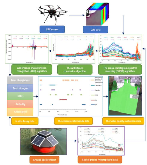
A set of technical processes of water quality parameter extraction is designed for the buoy spectrometer, UAV hyperspectral image data, and test data at sampling points (Figure 4). The cross-correlogram spectral matching (CCSM) algorithm can effectively match space and ground data (Section 3.2) and further improve the accuracy of UAV data (Section 4.1). A new absorbance characteristics recognition algorithm (ACR) (Section 3.3) is designed to compare the ground test data with the UAV data. This method can combine the advantages of the supervised and unsupervised approaches to select the overlapping band as the potential influential band for modeling (Section 4.2). Four scale amplification tests (Section 3.4) were carried out at the sampling points and the in situ scale to verify the scale effect, and the sensitive bands of water quality parameters at different scales are further studied. Using two-band cluster analysis (Section 3.4) and three regression algorithms (refer to Section 3.5 for the algorithm and Section 4.3 for the result), the accuracy evaluation results of five types of water quality parameters were obtained (refer to Section 3.6 for the algorithm and Section 4.4 for the result). The prediction results of five water quality parameters at modeling points were drawn. The distribution law of water quality parameters upstream, midstream, and downstream of the Lingnan Avenue River (Section 4.5) were analyzed based on these.

3.2. Spectral Matching Algorithm for UAV and Buoy Data

Since the sensor of the buoy spectrometer was only 10 cm away from the water surface and the spectral energy source was a stable halogen lamp, the water surface is considered a dark shaded environment, which can be recognized as the true reflectance of the water. Although the UAV spectrum was corrected by calibration cloth, some errors still occurred due to interference such as shadow occlusion and light intensity change. The cross-correlogram spectral matching (CCSM) algorithm [54] is used to calculate the linear correlation coefficient between buoy spectral data and UAV spectral data through the relative translation of the spectral axis and draw the cross-correlation coefficient diagram to remove these errors. It is considered that if the cross-correlation coefficient of the two bands reaches the maximum, it is a similar band. The secondary calibration of UAV spectral data is realized by this method.

This algorithm determines the similarity of the spectrum, which depends on the spectral shape rather than the reflectance, and can overcome the spectral error caused by atmospheric and sensor noise. It is susceptible to spectral shape error caused by the water surface structure. Matching two different spectral data to obtain a similarity value has always been one of the research focuses of hyperspectral remote sensing. The classical spectral angle matching algorithm is sensitive to the spectrum’s shape, but insensitive to the distance between the spectra. A binary coding algorithm is exposed to the characteristic spectral segments of the spectrum, but it cannot achieve high-precision spectral classification. Here, the cross-correlation spectrum matching algorithm (CCSM) is introduced, which can not only solve the problem of the relative shift of band but also suppress the interference of shadow and brightness and evaluate the similarity between the target spectrum and the reference spectrum. The CCSM algorithm calculates the correlation system, skewness, peak value, and correlation significance standard between spectral data. By calculating the cross-correlation coefficients of the target spectrum and the reference spectrum at different positions, and drawing the cross-correlation coefficient plot, we can judge the similarity of the two spectral data.

The formula for calculating the cross-correlation coefficient at the matching position m is:

$$r_m=\frac{n{\displaystyle \sum }\widehat{r_r}\widehat{r_t}-{\displaystyle \sum }\widehat{r_r}{\displaystyle \sum }\widehat{r_t}}{\sqrt{\left[n{\displaystyle \sum }\widehat{r_r^2}-{\left({\displaystyle \sum }\widehat{r_r}\right)}^2\right]\left[n{\displaystyle \sum }\widehat{r_t^2}-{\left({\displaystyle \sum }\widehat{r_t}\right)}^2\right]}}$$

(2)

where r_m is the cross-correlation coefficient, n is the number of bands where the two spectral data coincide, and m is the band matching position. m needs to be selected according to the complexity of spectral data. According to the test, the spectral data in this paper is taken as −20 to 20, which can be used to evaluate the spectral matching degree. When the value is 0, the band does not move; n is the number of bands where the two spectral curves coincide, $\widehat{r_r}$ is the spectrometer spectral, and $\widehat{r_t}$ is the UAV pixel spectral.

A continuous curve can be drawn by the cross-correlation coefficients of all matching bands’ positions [55]. The calibration is realized by expressing and comparing the difference between the spectral reference and the actually measured spectrum. The calculation formula for different degrees is:

$$RMS=\sqrt{\frac{{{\displaystyle \sum }}_{-m}^m{\left(\widehat{r_m}-r_m\right)}^2}{2·m+1}}$$

(3)

where RMS is the root mean square difference of the cross-correlation coefficient, $\widehat{r_m}$ is the cross-correlation coefficient curve of the buoy spectrum itself, and r_m is the cross-correlation coefficient curve of buoy spectral and UAV pixel spectral.

As m takes values from −20 to 20 in turn, a set of r_m values corresponding to each m is obtained through formula 2. RMS is calculated according to the cross-correlation coefficient by formula 3. R_m is the cross-correlation coefficient of the reference spectrum itself, and r_m is the cross-correlation coefficient of the reference spectrum and the target spectrum. Therefore, RMS is only sensitive to spectral type and shape and is not sensitive to error factors.

3.3. Absorbance Characteristics Recognition Algorithm (ACR)

Spectral feature selection can be divided into the unsupervised band selection method and the supervised band selection method according to whether there are chemical test data. The basic idea of the unsupervised band selection method is statistical spectral indicators, such as variance, information entropy, a signal-to-noise ratio, and the optimal index factor method. We estimate the importance of each band or between bands to the component content according to the differences between indicators. Generally, the method makes it difficult to improve the accuracy to a certain extent because of the lack of a specific purpose. On the other hand, the supervised band selection method achieves relatively better calculation accuracy based on specific training samples. Methods include regression analysis, principal component analysis, partial least squares, the support vector machine, and a neural network. The core purpose is to select a subset of bands with a number of D (d < D) from all wavelengths D of hyperspectral images by some search method to maximize the evaluation criterion function, regardless of which method is adopted.

An unsupervised band selection method for extracting water material content is designed. Absorbance reflects the sensitivity of each wavelength to water substances. The reflectance is converted to absorbance, the logarithmic ratio of the radiation incident on the water body to the radiation reflected by the water body. This conversion method can partly reduce the nonlinear noise problem of reflectance data [56]. The formula is:

$$A_i=\log 10\left(1/R_i\right)$$

(4)

where A_i is the absorbance value of band i and R_i is the reflectance value of band i.

A new index model is designed to select characteristic bands with no in situ value. The basic principle is to assume that spectral data are obtained at n sampling points. After calculating the absorbance using formula 4, values in the n spectral bands will be different for different samples. This difference is due to the different content of substances in water. In fact, after logarithmic transformation, the differences will be less dramatic; nevertheless, they will be more linearly related to the pigment concentration. An unsupervised band selection method, namely the absorption characteristics recognition algorithm (ACR), is innovatively designed. We compare the absorbance A_i of each band i of the water spectrum at different sampling points with the absorbance of the corresponding band i of the spectral data obtained at n sampling points. We select the standard deviation and average value as indicators to evaluate the deviation degree of absorbance at a single wavelength from the spectra of all sampling points. Various combinations of the absorbance, standard deviation, and average value are tested according to the classical method of statistics to ensure that the absorbance at different points has significant differences at specific wavelength positions. These particular positions are the characteristic bands that the ACR method pursues. It is found that the following combinations can aptly express this difference after hundreds of combinatorial experiments. It should be noted that when the absorbance of a specific wavelength is equal to the average absorbance of all sampling points, the denominator will be 0. This band should be discarded to ensure the calculability of the formula. The formula is:

$$S_i=\left[\left(A_i-S{D}_{A_i}\right)\times \left(A_i+AV{G}_{A_i}\right)\right]/\left[\left(A_i+S{D}_{A_i}\right)\times \left(A_i-AV{G}_{A_i}\right)\right]$$

(5)

where S_i is the calculated value of absorbance characteristics, A_i is the absorbance value of the band i, SD_Ai is the standard absorbance deviation of the band i, and AVG_Ai is the average absorbance of the band i. It is considered that the first 30 bands with the highest absorbance contain the information on the main pollutants in water quality according to the principle of unsupervised feature extraction. Therefore, these bands are selected for calculating the content of water pollutants as potentially independent variables.

The multiple linear regression techniques in the supervised band selection method are used to establish the correlation between each band and the content of the spectral at the sampling point. The formula is:

$$y=\left[\begin{array}{c}{y}_1\\ y_2\\ \dots \\ y_n\end{array}\right], X=\left[\begin{array}{c}1 x_{11}\dots x_{1i}\\ 1 x_{21}\dots x_{2i}\\ \dots \\ 1 x_{n1}\dots x_{ni}\end{array}\right],\beta =\left[\begin{array}{c}{\beta }_1\\ {\beta }_2\\ \dots \\ {\beta }_n\end{array}\right],ϵ=\left[\begin{array}{c}{ϵ}_1\\ {ϵ}_2\\ \dots \\ {ϵ}_n\end{array}\right]$$

(6)

where y_i is the chemical test data of each sampling point, X is the spectral reflectance value of the corresponding test point, β is the band coefficient value, and $ϵ$ is the intercept value. The correlation coefficients are sorted, and the first 30 bands are selected as the result of another characteristic band.

Comparing the results of unsupervised and supervised band selection methods, the overlapping bands are selected. These overlapping bands have an indicative relationship with the main indicators of water quality (Figure 5).

3.4. 5x Dimensionality Reduction Algorithm

The uncertainty of information extraction caused by the scale effect and the scale dependence of the extraction accuracy must be considered in calculating the surface parameters using hyperspectral remote sensing [57].

There are three main methods to obtain different scales of remote sensing data: (1) The sampling method, which expands the original image into a series of images with different resolutions through scale; (2) the multi-sensor method, which obtains the data of sensors with different resolutions in the same area, such as IKONOS pan 1 m, SPOT pan 20 m, TM 30 m, and MODIS 250 m; and (3) the variable altitude method, which obtains different-resolution data of the same sensor by adjusting the flight altitude. The three methods have advantages and disadvantages. For example, the sampling method will lead to the unreliability of the subsequent conclusions. Due to the different spectral response functions of sensors in the multi-sensor method, the work of a unified standard will also cause computational complexity in evaluating the scale effect. The variable altitude sensor is certain, so the data obtained with different resolutions have good comparability, but it is difficult to obtain. The improved sampling method is used to expand the spectral data from point data to five different levels of polygon data in this paper. Four adjacent pixels around the sampling point are taken as four scale levels. The number of pixels involved in the calculation is 1, 8, 16, 24, and 32, respectively (Figure 6). We take the spectral mean as the spectral value of each level.

There is a high correlation between adjacent bands of hyperspectral data [58]. A method integrating hierarchical and fuzzy clustering advantages is designed to realize the rapid band selection. The filtered band modeling can significantly improve the stability and prediction accuracy of the model and the extraction efficiency. Hierarchical clustering and fuzzy clustering algorithms are selected for feature band selection.

The steps of the hierarchical clustering method are as follows: (1) Calculate the distance between bands and combine the nearest bands into the same class; (2) calculate the distance between classes and merge the nearest classes; (3) repeat this process until all bands are merged into one class. The distance here is the Pearson correlation between bands. The greater the correlation, the smaller the distance and merge. The steps of the fuzzy clustering method are as follows: (1) The similarity matrix of the model is established according to the similarity coefficient method, and the value is between −1 and 1; (2) the transitive closure is established, and different level cut sets are obtained by transforming the fuzzy equivalent matrix; (3) the fuzzy similarity matrix satisfying transitivity is clustered by setting different confidence levels. Finally, the corresponding clustering bands are combined to complete the evaluation of characteristic bands after the two kinds of clustering are realized.

3.5. Regression Models

The multiple linear regression method (MLR), support vector machine method (SVM), and neural network (NN) method are selected to establish the regression model between water quality parameters and characteristic bands in this paper.

Generally, there is a linear correlation between water quality parameters and reflectance of the characteristic band, which is suitable for modeling with the multivariate linear model. The basic idea of stepwise multiple linear regression (MLR) is to gradually import all variables into the regression equation according to their importance and use F statistics to select or eliminate independent variables to establish the regression equation. The modeling method is as follows: Use the value of the F significance level as the criterion of the stepwise regression method to judge the relationship between the spectral data x and dependent variable water quality test value y during the analysis process and set the probability of selecting or eliminating independent variables to 0.05 and 0.10.

It is necessary to introduce a hyperplane to establish the regression relationship when the linear separability of the characteristic band decreases, and the support vector can play a powerful role in further improving the regression accuracy. The algorithm’s core aim is to map the output data to high-dimensional feature space by defining the kernel function and building an optimal classification hyperplane in space. Therefore, the algorithm can calculate the globally optimal result of water quality parameter prediction. EPS regression is chosen as the model category, linear linearity is selected as the kernel function, and the trial-and-error method is used to calculate the best gamma and penalty factor. Gamma is set to 10⁻⁵~10⁻¹, and penalty factors are selected to 10, 50, and 100. The error deviation of each combination is evaluated according to 20 iterations of cross-testing.

A neural network model is needed to participate in the calculation of a large amount of data, because a support vector machine is only suitable for the task of small-batch samples. Back-propagation neural networks are divided into three layers: An input layer, hidden layer, and output layer. Under the condition that the neuron response function is continuously differentiable, the back propagation of error is used to establish the model. The modeling method is as follows: Select the “S” function as the activation function of the neuron, and the output is

y = f² (w²f¹ (w¹x + b¹) + b²)

(7)

where y is the output layer of the predicted value of the water quality parameters, x is the input layer of the spectral data x, f¹ and f² are the transfer functions of the hidden and output layers, b¹ and b² are the deviations of the hidden and output layers, and w¹ and w² are the weights of the hidden and output layers.

3.6. Model Evaluation

R² (coefficient of determination) reflects the accuracy of model fitting data and represents the proportion of variance explained by the model. The range is 0 to 1. The closer to 1, the stronger the explanatory ability of the equation’s variables to y, and the better the model fits the data. Conversely, the closer to 0, the worse the model fits. For example, R² = 0.6 means that the model explains 60% of the uncertainty, and the model is acceptable. The R² coefficient calculation formula is as follows:

$$R^2=1-\frac{{{\displaystyle \sum }}_{i=1}^n{\left(y_i-\widehat{y_i}\right)}^2}{{{\displaystyle \sum }}_{i=1}^n{\left(y_i-\overline{y}\right)}^2}$$

(8)

where n is the sample size, $y_i$ is the assay value of the content of point i, $\widehat{y_i}$ is the content prediction value of spectral method of point i, and $\overline{y}$ is the mean of the assay value of the samples.

RMSE is the root mean square error in the same unit as the true value, ranging from 0 to infinity. For example, RMSE = 1 indicates that the average difference between the predicted value and real value is 1. When the expected value is entirely consistent with the real value, it is equal to 0, that is, the perfect model; the greater the error, the greater the RMSE value, and the worse the model. The calculation formula is as follows:

$$RMSE=\sqrt{\frac{1}{n}{{\displaystyle \sum }}_{i=1}^n{\left(y_i-\widehat{y_i}\right)}^2}$$

(9)

where n is the sample size, $y_i$ is the assay value of the content of point i, and $\widehat{y_i}$ is the content prediction value of the spectral method of point i.

4. Results

4.1. Space to Ground Matching Results

Comparing the average reflectance of 10 UAV strips with two buoy spectrometers, it is concluded that UAV spectra have more sensor noise, and the reflectance is more affected by illumination change than buoy spectrometers. The two buoy spectrometers have good similarities and consistent spectral patterns (Figure 7). The reflectivity is mainly affected by the weak liquid level (such as waves). UAV data have a great mutation in the first 5 bands and last 30 bands, indicating that they should not be selected as the characteristic bands in the subsequent modeling. The secondary calibration coefficient of each band spectrum is obtained according to the cross-correlation coefficient.

We draw the cross-correlation coefficient between the average reflectance of 10 UAV strips and buoys A and B, and Figure 8 reflects the change in the correlation coefficient when the spectral of the two devices move ±21. It can be concluded that (1) the positions of reflectance peaks and valleys of UAV spectral and buoy spectral are highly consistent. The correlation shows a downward trend in both positive and negative directions (Figure 8a,b). (2) It is necessary to evaluate the matching effect of UAV hyperspectral data and water surface spectral data because the river is divided into 10 sections for UAV data acquisition (that is, 10 strips). We try to select UAV data with a good matching effect for modeling. If the circle of the radar chart is larger and the shape is closer to the circle, it means that with the adjustment of the m value, the spectral data of the water surface spectrometer and the spectral data of the UAV match better. On the contrary, it shows that the UAV spectral data are more affected by shadow, atmosphere, or the correction algorithm. The cross-correlation coefficients of bands strip 7, strip 8, and strip 9 vary greatly, which shows that the spectral characteristics of these three bands are sensitive. When establishing the water quality calculation model, the characteristic bands selected on these three bands may not be robust (Figure 8c,d).

4.2. Water Quality Parameters Characterization Band Set

The reflectance data of 272 bands at each position are collected according to the longitude and latitude of the sampling point. Here, the data with five water quality parameters, namely, the sampling point data of total phosphorus, total nitrogen, COD, turbidity, and chlorophyll, are defined as effective data. On the hyperspectral images of strips 1 to 10, there are 11, 4, 4, 2, 2, 2, 2, 2, 5, and 2 valid data, respectively. Buoy A and buoy B have four and five valid data, respectively. So, a total of 45 groups of valid data are formed (Figure 9a). It is concluded that the spectral data of the same strips have great similarity, indicating that the water quality at a similar distance is also similar. The spectral sampling points of different strips are significantly different, which is a favorable phenomenon for subsequent modeling. The sensor has obvious noise at both ends, including 400 nm to 410 nm and 920 nm to 1000 nm.

It is considered that as long as the wavelength of light is fixed, the absorption coefficient of the same substance will remain unchanged according to the principle that the absorption coefficient is related to the wavelength of incident light and the substance passed by light [59]. This phenomenon is very suitable to be used for the material content calculation. We take 10 as the base and 100 as the parameter to convert the absorbance of the spectrum to obtain the ratio of incident light to transmitted light on the water surface (Figure 9b). It is concluded that the absorbance increases significantly with the increase in wavelength. The longer the wavelength, the more energy the water absorbs. If this trend is not maintained, it is caused by the material composition of the water body. The corresponding band can be selected to retrieve its material content.

We calculate the absorbance characteristic bands (Figure 9c) according to Formula (5) and sort the characteristic bands of each sampling point after calculating the absolute value. The spectral data corresponding to 45 sampling points have 45 sorting possibilities. The first 30 bands are selected as the final result of unsupervised characteristic band selection according to the principle of maximum simple addition value (Figure 9d). It can be seen that there is no participation of any chemical test data in the whole process. The results of the calculation are 785 nm, 747 nm, 727 nm, 781 nm, 774 nm, 787 nm, 725 nm, 776 nm, 783 nm, 803 nm, 805 nm, 809 nm, 754 nm, 778 nm, 678 nm, 730 nm, 794 nm, 758 nm, 772 nm, 798 nm, 745 nm, 736 nm, 790 nm, 750 nm, 421 nm, 743 nm, 741 nm, 674 nm, 767 nm, and 416 nm.

We analyze the correlation between the contents of five water quality parameters and the full wavelength to obtain the band number of the top 30 in the positive correlation and negative correlation (Figure 10a). Spectroradiometer noise at wavelengths on both limits of their spectral range is common (its cause is often the low signal-to-noise ratio and low solar irradiation at those wavelengths combined with higher sensitivity of the detectors to operating temperature). So, the first 10 bands (400 nm to 420 nm) and the last 30 bands (920 nm to 1000 nm) are removed when selecting the characteristic band due to the interference of instrument noise. The correlation coefficient of COD and chlorophyll is generally high, reflecting that the extraction accuracy may be higher. (1) There was a negative correlation between total phosphorus and all bands, and the correlation coefficient ranged from −0.116 to −0.460. (2) There was a negative correlation between total nitrogen and all bands, and the correlation coefficient ranged from −0.116 to −0.460. (3) COD showed a positive correlation with all bands, and the correlation coefficient ranged from 0.303 to 0.416. (4) Turbidity has a negative correlation with 420 nm to 700 nm, and a positive correlation with subsequent bands, with correlation coefficients ranging from −0.282 to 0.094. (5) Chlorophyll showed a positive correlation with all bands, and the correlation coefficient ranged from 0.078 to 0.384.

We overlay the characteristic bands selected by the correlation coefficient method with the characteristic bands selected by the unsupervised method (Figure 10b). It is considered that the overlapping wavelength region can improve the calculation accuracy of water quality parameters to the greatest extent because both supervised and unsupervised methods select it. The characteristic band sets of total phosphorus are 425 nm to 434 nm, with a total of five bands. The characteristic band sets of total nitrogen are 671–682 nm and 694–711 nm, with a total of 15 bands. The characteristic band sets of COD are 700 nm, 722–736 nm, and 765–771 nm, with a total of 12 bands. The characteristic band sets of turbidity are 427–434 nm and 773–778 nm, with a total of seven bands. The characteristic bands of chlorophyll are 425–434 nm, with a total of three bands.

4.3. Response of Sensitive Bands to Water Quality Content at Different Scales

The effect intensity of the scale effect is preliminarily judged by cluster calculation. The clustering results of 272 bands in five scales are obtained according to the two algorithms Section 3.5. The results show that the category identification positions are 521 nm, 656 nm, 721 nm, 829 nm, 929 nm, and 963 nm, respectively (Figure 11). The results of clustering under different scales have great similarities, except for fuzzy clustering at 16 scales. In addition, the similarity is also reflected in the merging of short waves and long-waves with the change in wavelength at all scales. Spectral data of different wavelengths are combined into five categories after two clustering methods. The same color indicates that the clustering results are one class. Although the red and blue band ranges in Figure 11 are discontinuous, they can be aggregated into one type of spectral data. These phenomena imply that it has little effect on the extraction accuracy of water quality parameters under the current five scale divisions. The underlying reason that the scale effect can be ignored is that the spatial resolution of UAV hyperspectral is very high, and the river channel is relatively narrow.

The relatively best regression methods of different water quality indicators appear on different scales (

Table 2. Regression results for the water quality parameters.

Scale	Method	Accuracy	TP	TN	COD	Turbidity	Chlorophyll
1 *	ACR	RMSE	0.2113	3.4244	3.9972	7.0520	0.0062
		R2	0.6142	0.3201	0.1673	0.3054	0.1431
	MLR	RMSE	0.1799	2.5217	3.7454	5.5209	0.6104
		R2	0.3698	0.4276	0.2688	0.5742	0.0900
1	SVM	RMSE	0.1858	2.9075	3.3585	7.5495	0.5614
		R2	0.3684	0.2532	0.4274	0.2139	0.2638
	NN	RMSE	0.2024	2.9117	4.0375	6.7541	0.4725
		R2	0.2026	0.2369	0.1502	0.3628	0.4546
8	MLR	RMSE	0.1820	1.0607	3.7279	3.9585	0.4787
		R2	0.3277	0.7949	0.2866	0.7105	0.4431
	SVM	RMSE	0.1762	2.0915	3.5193	5.6504	0.4778
		R2	0.4400	0.2078	0.3837	0.4796	0.4648
	NN	RMSE	0.2223	3.2793	2.6825	8.4609	0.5512
		R2	0.0381	0.0320	0.6249	0.1279	0.2578
16	MLR	RMSE	0.1767	1.0815	3.8211	6.1119	0.4391
		R2	0.3657	0.7868	0.2504	0.3100	0.5313
	SVM	RMSE	0.1867	1.9938	3.6679	6.3852	0.4730
		R2	0.3241	0.2857	0.3376	0.3467	0.4798
	NN	RMSE	0.2218	3.2981	3.9968	8.4518	0.6190
		R2	0.0422	0.0208	0.1673	0.0022	0.0640
24	MLR	RMSE	0.1741	2.3017	3.7519	5.3045	0.4488
		R2	0.3845	0.0341	0.2774	0.4802	0.5104
	SVM	RMSE	0.1912	1.9701	3.6856	6.3527	0.4832
		R2	0.2775	0.3201	0.3299	0.3429	0.4607
	NN	RMSE	0.2055	3.3055	4.0253	7.1815	0.5828
		R2	0.1776	0.0165	0.1554	0.2796	0.1705
32	MLR	RMSE	0.1772	1.1327	3.8439	5.1770	0.3907
		R2	0.3624	0.7662	0.2415	0.5049	0.6289
	SVM	RMSE	0.1866	1.9808	3.6631	6.4209	0.4725
		R2	0.3215	0.2941	0.3408	0.3434	0.4813
	NN	RMSE	0.2189	3.3162	4.0816	8.4297	0.6094
		R2	0.0673	0.0101	0.1316	0.0074	0.0929

* The ACR method has only scale 1 data.

):

(1) The ACR method only has the highest R² value (0.6142) in the calculation of total phosphorus, although the ACR method combines the characteristic bands selected by supervised and unsupervised methods. The RMSE value of the ACR method is the smallest in chlorophyll calculation, but considering that R² is only 0.1431, it cannot be selected as the final calculation model.

(2) Surprisingly, the MLR, SVM, and NN methods did not reach the highest R² and lowest RMSE when calculating all water quality indicators at scale 1 after comparing the regression results of all five scales. On the one hand, it shows that only one pixel is selected in the quantitative calculation of hyperspectral data, which cannot represent the real situation of the water environment. On the other hand, it is impossible to calculate an accurate water quality index because the selected pixel is not necessarily the point of collecting water samples due to the inherent error of GPS positioning (0.5–1 m).

(3) Scale 8 is a relatively balanced amount of data relative to the other four scales. The highest R² is reached in the calculation of total nitrogen, COD, and turbidity, which are 0.7949, 0.6249, and 0.7105, respectively, and RMSE is also the lowest in all results, which shows a good calculation effect under this scale.

(4) The calculation results of scale 16 and scale 24 are similar to that of scale 1. There are no higher R² and lower RMSE in the calculation results of the other three methods, except the RMSE of total phosphorus on scale 24 is 0.1741 (ranking first, but R² is only 0.3845) and the R² of total nitrogen in scale 16 is 0.7868 (ranking second). However, the reason for this phenomenon is significantly different from scale 1. It is more because the typical characteristic position of reflectance is not significant, which is caused by excessive spectral averaging.

(5) The R² of chlorophyll reached 0.6289, which was significantly higher than that of ACR and the other four scales with the scale enlarged to 32. In addition, the R² of TN is also as high as 0.7662 (ranking third). This phenomenon is because chlorophyll is evenly dispersed and fully mixed in the water body. Similarly, TN is the collection of various nitrogen elements such as ammonia nitrogen, nitrogen, and nitrogen oxide in water. Therefore, the scale enlargement can also extract more accurate results.

Comparing ACR, MLR, SVM, and NN4 calculation methods, the conclusions are as follows: (1) The ACR method of total phosphorus and the MLR method of total nitrogen, turbidity, and chlorophyll reached the highest value of R² on the corresponding scale (Figure 12a). The ACR method of chlorophyll and the MLR method of total phosphorus, total nitrogen, and turbidity reached the minimum value of RMSE on the corresponding scale, respectively (Figure 12b). (2) The SVM method does not reach the relative maximum of R² (Figure 12c) and the relative minimum of RMSE (Figure 12d) on all scales, which shows the shortcomings of this method. (3) The COD regression coefficient R² of the NN method reaches the relative maximum (Figure 12e), and the RMSE of COD calculated by the NN method reaches a relative minimum (Figure 12f) at scale 8, which indicates the best method and scale of COD.

4.4. Accuracy Evaluation

According to the response of sensitive bands to water quality content at different scales (Section 4.3), the scale 1 data of the ACR method are chosen to calculate the total phosphorus content, the scale 8 data of the MLR method are selected to calculate the total nitrogen and turbidity, the scale 8 data of the NN method are selected to calculate the COD, and the scale 32 data of the MLR method are selected to calculate the chlorophyll.

The accuracy of data is limited in terms of sampling points. According to the definition in Section 4.2, there are 45 valid datasets. The water samples of 9 points are collected at buoy A and buoy B positions among the 45 sampling points. These points had no spectral data (only buoy pixels) on the UAV image, and 20 sampling points appeared on the adjacent UAV strips and were merged (after merging, 10 data were left). Therefore, there are a total of 26 groups of data that can be used to compare the measured value with the predicted value. These data appear to have trends different from the Y = X line because the number of sampling points is generally small, and there are individual extreme values. The accuracy of COD (Figure 13a) and turbidity (Figure 13b) is low comparing the calculation results of five water quality parameters. COD data generally need to be obtained by testing for several consecutive days. The test data only include single-time data, which cannot reflect the actual situation of water quality COD. Turbidity should reflect the comprehensive situation within a specific water depth and thickness, which is difficult to calculate for hyperspectral data. The comparison accuracy of total phosphorus, total nitrogen, and chlorophyll are 0.6925 (Figure 13c), 0.7291 (Figure 13d), and 0.7658 (Figure 13e), respectively, which is acceptable.

4.5. Mapping and Water Quality Evaluation

The river in the study area flows slowly from north to south, and the velocity is lower than 0.1 m/s under normal conditions. Some river sections have weak backflow, and the overall hydrological situation is similar to that of inland lakes, which is conducive to the hyperspectral work. The results showed that the content of total phosphorus changed gently, ranging from 0.4061 mg/L to 2.0605 mg/L (Figure 14a). The content of total nitrogen changed sharply, ranging from 0.1323 mg/L to 109.8340 mg/L. The content of COD changes violently, ranging from 0.0251 mg/L to 48.3270 mg/L. The content of turbidity changes very sharply, ranging from 1.8461 to 3248.6800. The content of chlorophyll also changed sharply, ranging from 0.0878 mg/L to 338.2971 mg/L by calculating five water quality parameters of the river. The pollutant content of the whole river shows a great difference. The reasons are as follows: On the one hand, the river channel is narrow (the narrowest part is less than 5 m) and the flow velocity is slow, and many piers lead to the accumulation of pollutants. On the other hand, there are many urban commercial and domestic sewage outlets, and all kinds of contaminants show a sharp increase near the sewage outlets.

Four typical areas are selected, which are the starting point (No. 1), catchment (No. 2), direct flow (No. 3), and end point of the river (No. 4). Different areas show different laws (Figure 14b). (1) The river presents the state of pollutant accumulation on the north bank due to the inflow of the upstream mainstream river at the starting point of the river. The other four pollutants increase significantly, except the total nitrogen law is insignificant. This phenomenon reflects that a large part of the pollutants in the river come from the upstream mainstream river. (2) The river channel leaks out of the ground again, and all kinds of pollutants show explosive growth under the combined action of chemistry and physics at the catchment. Moreover, the river here is narrow, which causes the water to present the characteristics of a typical black odor water body. (3) The river enters a downstream state of hundreds of meters, and the concentration of pollutants decreases significantly at the direct current. A pollutant strip appears west of the center of the river due to the action of water flow. Moreover, two circular high-value areas of pollutants can be seen, and it can be inferred that there are underwater sewage outlets at these two locations. It is speculated that there are two aquatic sewage outlets because two circular high-value areas of pollutants can be seen. (4) Various pollutants are fully diluted and reduced at the end of the river. On the one hand, there is a large area of open water downstream, which has a significant scouring effect. At the same time, the relative concentration of pollutants is significantly reduced after a certain flow distance due to the river’s degradation ability.

The river hyperspectral image data are divided into downstream, midstream, and upstream sections according to the distribution of 10 bands (Figure 15). The calculation shows that the total phosphorus content in the upstream and midstream is low, ranging from 0.4061 mg/L to 1.6528 mg/L, and there is a high value in the upstream, reaching 2.0605 mg/L (Figure 16a). The distribution of total nitrogen in the three river sections is close (Figure 16b). The minimum value is 0.1323 mg/L downstream, and the maximum value is 109.8340 mg/L in the midstream. The COD content in the downstream reaches is significantly higher than that in the upstream and midstream, up to 48.3270 mg/L (Figure 16c). The three river sections show a trend of gradual reduction of COD, which is in line with the objective law of COD. The turbidity in the midstream is significantly higher than that in the upstream and downstream, with a peak of 3248.6800 JTU (Figure 16d). This river section combines all kinds of pollutants from upstream. At the same time, the purification capacity of the river has not played a significant role, resulting in such high turbidity. There is no significant watershed difference in the distribution of chlorophyll, but it has a great correlation with the content of total phosphorus and total nitrogen, reflecting the promotion effect on aquatic algae due to water eutrophication (Figure 16e).

5. Discussion

On the one hand, UAV hyperspectral has the characteristics of high efficiency, flexibility, rich information, and accurate acquisition of ground feature data. Urban inland river water quality survey is one of the important works of urban environmental protection. Assessing the major water pollutants based on UAV hyperspectral is not only a practical need of modern urban management but also the inevitable result of the development of hyperspectral technology. On the other hand, the processing and application of hyperspectral data of the UAV cannot meet the needs of regular, long-duration, and rapid applications. Therefore, deploying hyperspectral instruments that can work for 24 h on the water surface has become a good complementary means to the UAV.

Therefore, based on the hyperspectral remote sensing data of UAV, we selected the key characteristic bands through two ideas of supervision and unsupervised methods by using the hyperspectral buoy instruments and some in situ test data. First, a set of matching algorithms of UAV spectral data is designed. These algorithms play a good role in improving the accuracy of hyperspectral data of the UAV. Furthermore, a new algorithm (ACR) is developed. The algorithm can select the potentially valuable band data of spectral data without the support of laboratory data. These data reflect the action degree of the main pollutants in the water body.

Modeling based on in situ assay data is still studied to verify this method’s effectiveness. Results have proved that the two methods obtained at least three or more overlapping bands. In terms of modeling methods, the classical multiple linear regression, support vector machine, and neural network methods are selected to calculate the water quality parameters of the selected characteristic bands. One difficulty is that UAV data are polygon data, while laboratory data are spatial point data. Therefore, the number of pixels that should be selected to compare the two becomes a problem. Here, a pixel with a 0.2 m resolution is reduced to five scales of data. According to the evaluation of two clustering methods, the conclusion is that with such high-spatial-resolution data, the scale effect is not a significant factor, and the real cause of spectral changes is the material composition of the water itself. This idea is essential for subsequent research.

Finally, a series of conclusions are drawn, including the best modeling method, the best modeling scale, and the highest calculation accuracy of the five water quality parameters. Focusing on the two difficulties of quantitative recognition of UAV hyperspectral data and effective hyperspectral matching between UAV and ground data, the research process is studied. This systematic research realizes the fusion of hyperspectral data of UAV, hyperspectral data of water surface, and in situ test data. It also realizes the integration of data acquisition and field investigation. These works have promoted the development of digital water quality investigation towards intellectualization and the advancement of digital intelligent environmental protection. With the maturity of the technology, the new technology in the field of water quality investigation will develop in the direction of informatization, objectification, and intelligence.

6. Conclusions

The future water environment monitoring work will show the characteristics of high data fusion of multiple platforms. In this paper, a new remote sensing monitoring mode of water quality is designed and implemented: A buoy spectrometer with continuous working ability on the water surface and a flight platform for large-area synchronous monitoring in the air. The conclusions are as follows: (1) The data of the flight platform are limited by atmospheric interference, shadow, and pixel resolution, which needs the calibration of the water surface spectrometer. The airborne spectral data will be more real through simple coefficient conversion, which is the fundamental guarantee for the calculation accuracy of water quality. (2) The traditional characteristic band selection method is based on the correlation between reflectivity and content. Although a large number of algorithm tests have been carried out, the applicability has been questioned due to the inherent limitations of the water optical model. A band selection algorithm (ACR algorithm) with reflectivity related to content and strong absorbance characteristics is proposed, which improves the accuracy of calculation results to a certain extent, especially in the extraction of total phosphorus and chlorophyll. (3) Spatial–spectral differences should be fully considered when comparing test data for hyperspectral data combination of spectroscopy and optical imaging. The reason is the best results of different water quality parameters appear on different scales. This scale effect has a certain relationship with the algorithm, which leads to a relatively complex problem. This paper conducted a preliminary exploration. The research results not only have scientific reference significance for the processing and analysis of point and polygon hyperspectral data but also provide a complete solution for the monitoring and treatment of small watershed rivers in urban areas.