
On-Orbit Characterization of TanSat Instrument Line Shape Using Observed Solar Spectra
by

Zhaonan Cai
1,2, 
Kang Sun
3,4,
Dongxu Yang
1,2,*,
Yi Liu
1,2,5,
Lu Yao
1,2,
Chao Lin
6 and
Xiong Liu
7 1
Carbon Neutrality Research Center, Institute of Atmospheric Physics, Chinese Academy of Sciences, Beijing 100029, China
2
Key Laboratory of Middle Atmosphere and Global Environment Observation, Institute of Atmospheric Physics, Chinese Academy of Sciences, Beijing 100029, China
3
Department of Civil, Structural and Environmental Engineering, University at Buffalo, Buffalo, NY 14260, USA
4
Research and Education in Energy, Environment and Water Institute, University at Buffalo, Buffalo, NY 14260, USA
5
University of Chinese Academy of Sciences, Beijing 100049, China
6
Changchun Institute of Optics, Fine Mechanics and Physics, Changchun 130033, China
7
Center for Astrophysics|Harvard & Smithsonian, Cambridge, MA 02138, USA
*
Author to whom correspondence should be addressed.
Remote Sens. 2022, 14(14), 3334; https://doi.org/10.3390/rs14143334
Submission received: 24 May 2022
/
Revised: 1 July 2022
/
Accepted: 5 July 2022
/
Published: 11 July 2022
(This article belongs to the Special Issue China's First Dedicated Carbon Satellite Mission (TanSat))
Abstract
:The Chinese carbon dioxide measurement satellite (TanSat) has collected a large number of measurements in the solar calibration mode. To improve the accuracy of XCO2 retrieval, the Instrument Line Shape (ILS, also known as the slit function) must be accurately determined. In this study, we characterized the on-orbit ILS of TanSat by fitting measured solar irradiance from 2017 to 2018 with a well-calibrated high-spectral-resolution solar reference spectrum. We used various advanced analytical functions and the stretch/sharpen of the tabulated preflight ILS to represent the ILS for each wavelength window, footprint, and band. Using super Gaussian+P7 and the stretch/sharpen functions substantially reduced the fitting residual in O A-band and weak CO band compared with using the preflight ILS. We found that the difference between the derived ILS width and on-ground preflight ILS was up to −3.5% in the weak CO band, depending on footprint and wavelength. The large amplitude of the ILS wings, depending on the wavelength, footprint, and bands, indicated possible uncorrected stray light. Broadening ILS wings will cause additive offset (filling-in) on the deep absorption lines of the spectra, which we confirmed using offline bias correction of the solar-induced fluorescence retrieval. We estimated errors due to the imperfect ILS using simulated TanSat spectra. The results of the simulations showed that XCO2 retrieval is sensitive to errors in the ILS, and 4% uncertainty in the full width of half maximum (FWHM) or 20% uncertainty in the ILS wings can induce an error of up to 1 ppm in the XCO2 retrieval.
1. Introduction
The Chinese carbon dioxide measurement satellite (TanSat) is the first Chinese hyperspectral satellite dedicated to observing the column-averaged CO dry-air mole fraction (XCO2) and constraining the regional carbon flux inversion [1]. TanSat was launched in December 2016 into a 700-km sun-synchronous orbit with an equator crossing time of 13:30 h. It carries two instruments, the Carbon Dioxide Sensor (CDS) and Cloud and Aerosol Polarization Imager (CAPI). The CDS, similar to the OCO-2 instrument [2], incorporates three grating spectrometers operating in the O A-band (758–778 nm), weak CO band (1594–1624 nm), and strong CO band (2042–2082 nm) [3]. The CDS measures reflected sunlight off the Earth for measurements of atmospheric constituents and direct sunlight for calibration purposes. The CAPI is a five-band imager with two polarization channels providing information on aerosol optical properties [4]. The radiometric calibration (dark current response, gain coefficients, and signal-to-noise ratio), spectral registration, and instrument line shape (ILS) of the TanSat CDS instrument were characterized and experimentally determined on the ground [5,6].
To improve the retrieval accuracy, the spectral calibration (e.g., ILS and wavelength calibration) must be accurately determined, and the contribution of their uncertainties to the total error budget must be understood. The results of simulations showed that methane retrieval is sensitive to errors in ILS, and an accuracy of 1% of ILS is required [7] to meet the retrieval accuracy of the TROPOspheric Monitoring Instrument (TROPOMI). The knowledge of the ILS, or slit function, is required, in the forward model, to convolve the reference spectrum and simulate the radiance spectrum from high spectral resolution to the resolution of the instrument, which is the common practice for current trace gas retrieval algorithms. For grating instruments, such as TanSat and OCO-2, the ILS and the spectral dispersion for each spectral pixel, footprint, and band was characterized by scanning tunable diode lasers experiment [6,8]. However, simple functions are unable to represent these ILSs. Instead, a lookup table was calculated to describe the ILS. This is in contrast to TROPOMI, which models the ILS by a function of eight parameters describing the peak and tails [9].
TanSat is dedicated to retrieving the XCO2 with a precision of 1–4 ppm [3]. Retrieval algorithms based on optimal estimation [10,11] and the IMAP-DOAS algorithm [12] have been developed. These algorithms perform additional spectral and radiometric calibration prior to the spectral fitting. Validation against ground-based FTIR measurements from TCCON showed good agreements between TanSat and TCCON, with standard deviations ranging from 1.47 to 2.45 ppm for different algorithms. These algorithms use the preflight tabulated ILS [10] or a super-Gaussian function derived through a cross-correlation of the measured solar spectrum to a high-resolution solar reference spectrum [12]. However, the precalibrated ILS could be changed due to the vibration during launch, orbital movement, thermal variation and instrument degradation; fitting a different ILS function form may induce artificial error due to the undersampling effect [13]. Therefore, the post-launch ILS of TanSat must be characterized.
This paper is organized as follows: We describe the TanSat instrument and measurements we used for ILS characterization in Section 2. The ILS functions used for fitting and the fitting algorithm are also presented in this section. The on-orbit spectral and temporal variations of ILS are presented in Section 3. Section 4 describes the evaluation of the effect of ILS on SIF and XCO2 retrievals. Finally, Section 5 summarizes this study.
2. Data and Method
2.1. TanSat Instrument and Data
The Carbon Dioxide Sensor (CDS) onboard TanSat measures sunlight in the near-infrared band that is back-scattered and reflected off the Earth’s surface on top of the atmosphere. The satellite can operate in three Earth observation modes: nadir (ND) over land, glint (GL) over the ocean, and target (TG) over calibration sites. The CDS instrument includes three push-blooming grating spectrometers, which cover the 0.76 µm band (O2A), two CO bands at 1.61 and 2.06 µm (WCO2 and SCO2) with resolving powers of 19,000, 12,800 and 12,250, respectively. The swath of footprint is about 20 km and the spatial resolution is 2 × 2 km. A pointing mirror made of aluminum was designed to reflect incident light to the telescope by the front side, and the back side was used as a reflected diffuser for onboard solar calibration. Preflight radiometric calibration (e.g., dark current, gain, signal-to-noise ratio) was performed [5].
The spectrometer of the O2A band uses a 1252 × 1152 array detector. In the spectral dimension, 1242 out of 1252 pixels are used. In the spatial dimension, 288 out of 1152 pixels are used, and 32 pixels are coadded into one pixel. Thus, 9 spatial footprints are taken across the track. For the spectrometer of two CO bands, 500 × 256 array mercury cadmium telluride (MCT) detectors are used, with 500 pixels in the spectral dimension and 216 pixels in the spatial dimension. A total of 24 pixels are coadded in the spatial direction; thus, two CO bands had 9 spatial footprints.
TanSat measures solar spectra in Sun-observation mode once per day at the terminator in the Northern Hemisphere when the satellite flies at the end of ascending for each orbit. A regular solar observation lasts for approximately 7 min (1260 frames). The solar calibration starts before the Sun is fully in the field-of-view of the diffuser and ends after the Sun has moved into the shadow of the Earth. As a consequence, limb measurements of the upper atmosphere are recorded during the Solar calibration. In the calculation of each solar mean spectrum, only those measurements with a solar zenith angle within 90 ± 1.5 (170 frames) are used to avoid Earthshine contamination. Note that the boresight zenith angles are rotated by 5 degrees to avoid damaging another CAPI instrument. Unlike OCO-2, no solar calibration measurements of the entire dayside of an orbit are recorded; thus, no oversampled solar Doppler measurements for TanSat. The Doppler effect causes the spectral features in the observed solar spectrum to be red-shifted because the satellite is moving away from the Sun, which is corrected using the relative speed of the satellite and Sun. Figure 1 shows an example of a TanSat solar mean spectrum. Note that we simply scaled the reference solar spectrum to the TanSat measurements. Below you will also see the fitting residuals for each band. Observations with OCO-2’s onboard solar measurements have indicated a degradation in the sensitivity of the oxygen spectrometer, which is mainly attributed to the contamination of the detector. Similar contamination-induced degradation was also found in the GOME and GOME-2 instruments [14,15]. The daily mean solar spectra of TanSat are normalized to the Sun-Earth distance and solar measurements at the beginning of the mission for degradation analysis (not shown here). The O2A and WCO2 bands degrade little over time after one year of operation (the signal had varied less than 0.5%), while in SCO2 band, the signal degrades by less than 2.5%.
A slightly curved entrance slit is used for each spectrometer to correct the smile effect. The preflight ILS and spectral dispersion are determined by fitting the measurements obtained by the three tunable diode lasers that scan the three bands. The spectral ranges covered by lasers were approximately 758.2–777.2, 1592.8–1624 and 2040.3–2076.7 nm, with step sizes of 0.005, 0.015, and 0.02 nm, respectively. A fifth-order polynomial is used for wavelength registration, with coefficients varying with footprints. Tabular ILS functions for each band are given in the level 1B data, with cut-off wavelengths of 0.235, 0.7 and 0.925 nm, respectively. The FWHM values of the spectral pixels are in the range of 0.0392–0.0424, 0.123–0.128 and 0.157–0.168 nm for O2A, WCO2, and SCO2 bands, respectively [6]. The precalibrated ILS is used in the XCO2 and SIF retrieval algorithm, and wavelength registration is calibrated using the solar Fraunhofer lines of the measured solar spectra [10,16]. Figure 2 shows examples of TanSat ILSs of nine footprints for three bands. The TanSat preflight ILSs of the O2A band behave similarly to those of OCO-2 ILS. Asymmetry was found in all three bands, in particular, in the ILS wings of the SCO2 band.
2.2. ILS Functions and Fitting Algorithm
Several types of analytical functions have been tested to model the ILS of OCO-2 [13,17], for example, hybrid Gaussian, super Gaussian, and their asymmetric forms; please refer to Sun et al. [13] for more details on these formulas. However, the wings cannot be fully represented by these analytical functions. The TROPOMI SWIR ILS is modeled by the weighted sum of a skew-normal-convolved-with-uniform function and a Pearson type-VII distribution, with the former capturing the peak and the latter capturing the tail that relates to the spectral stray light [9]. In this study, for TanSat ILS, we tested an ILS function similar to TROPOMI but using a super Gaussian for the peak (hereafter referred to as super Gaussian+P7; the blue lines in Figure 3 provide examples of the shape of this function for three bands) because it is easier to implement and interpret. The peak, tail, and ILS formulas are given by:
where controls the width of peak and, largely, the FWHM of the entire ILS; k controls the flatness of the peak; a controls the asymmetry of the peak; controls the relative contribution between the peak and the tail; m controls the steepness of the tail; is the FWHM of the tail.
We also tested the stretch/sharpen approach [8,13], which refines the preflight ILS by two parameters, and . The stretch term scales the ILS in the axis, then FWHM is scaled as a consequence. The sharpen term determines the shape of the entire ILS with power , which raises the relative amplitude of the wings and keeps the FWHM unchanged (see Figure 3 for illustrations):
These parameters of ILS functions can be determined through a nonlinear least squares (NLLS) fitting of the observed and simulated solar spectra. The simulated solar spectrum is modeled by convolving the high-resolution solar reference spectrum with ILS functions:
where denotes the high-resolution solar reference; denotes the ILS function defined at calibrated wavelengths . The is a fourth-order polynomial that scales reference to the measurements. Zero-order wavelength shift and squeeze are also fitted.
The high-resolution solar reference spectrum is obtained from the solar reference spectrum generated from version 2016 of the disk-integrated solar pseudo-transmittance spectrum [18] and a solar continuum spectrum [19]. The current TanSat L2 retrieval algorithm also uses the solar line list and solar continuum spectrum scaled to the observed solar spectrum [10]. We also tested the version 2020 solar line list and TSIS-1 Hybrid spectrum, which covers 202–2730 nm at 0.01–0.001 nm spectral resolution with uncertainties of 0.3% between 460 and 2365 nm [20]. The 2020 version of the solar line list does not improve the fitting. Using the TSIS spectrum only slightly improves the fitting residual in the O2A band, and the difference between using TSIS and the version 2016 line list is negligible for SCO2 and WCO2 bands. The number of solar Fraunhofer lines is limited in TanSat windows, so each band is divided into several subwindows for fitting, following the previously described method Sun et al. [13] (the wavelength range of each sub-window is shown below). The sparseness of solar lines in O2A and SCO2 bands makes it more difficult to derive super Gaussian+P7 parameters. Not all of the five parameters can be retrieved at the same time when only a few lines exist in a sub-window because the asymmetry term, wavelength shift, , and m are competing for the information. and m make it more complicated in that the fitting sometimes cannot converge due to the small signal of the tails. To overcome this problem, two-step fitting, similar to that previously reported [9], is performed. First, and m are derived using the full band, assuming that they are wavelength-independent. Second, the convergence of the sub-window fitting can be achieved by fixing and m, and the tail fraction and other parameters are fitted.
Figure 3 compares the retrieved ILS using three different ILS functions with preflight ILS for O2A, WCO2, and SCO2 bands. Both the stretch/sharpen and super Gaussian+P7 function show raised wings compared to the preflight ILS (for example, are derived as 0.83, 0.82, and 0.9, respectively), indicating a possible stray-light effect and will increase the effectiveness of the ILS far-wing response. ILS is sensitive to this signal. The asymmetric super Gaussian function can not capture the tails.
3. ILS Calibration
3.1. Spectral Variation in ILS
The ILS functions are derived for each footprint and each day with acquired solar calibration measurements. Figure 4 shows an example of the fitting results at footprint 1 on 1 March 2017. Figure 4a–c shows the FWHM of four ILS functions at the median wavelengths of each fitting window. The FWHMs derived using stretch/sharpen and super Gaussian+P7 function show wavelength-dependent structures similar to the preflight ILS, and they agree well in the O2A band. The asymmetric super Gaussian function behaves differently due to the shape mismatch. For the O2A and WCO2 bands, the derived FWHMs are generally smaller than those of the preflight ones, particularly in the WCO2 band. The middle panel (Figure 4d–f) shows the average fitting residuals at each fitting window when using four ILS functions. The fitting residual using four ILS functions shows similar spectral variations.
There is a noticeable improvement in the fitting residuals in both the O2A and WCO2 bands by adjusting ILS using stretch/sharpen and super Gaussian+P7 function. Adjusting the ILS and wavelength shift reduces the average residuals to 0.17% for the O2A band and 0.15% for the WCO2 band, particularly at the lower and upper wavelength ends of the WCO2 band. The fitting residual using the super Gaussian+P7 function generally agrees well with or slightly better than that obtained using the stretch/sharpen function. Using the derived ILS function only slightly reduces the fitting residual in the SCO2 band. Using an asymmetric super Gaussian function does not improve the fitting residual for any of the three bands, indicating the necessity of including tails. Similar to Figure 4d–f, Figure 4g–i shows the fitting residual at each wavelength. Substantial improvements at specific solar lines can be achieved by using the derived stretch/sharpen or super Gaussian+P7 function at O2A and WCO2 bands. The oscillating structure remains in the spectrally resolved fitting residual. Yang et al. [10] apply a Fourier decomposition approach to capture and correct these structures in solar spectral calibration, cloud screening and XCO2 retrieval and attribute these wave-like patterns to the radiance response calibration. These structures behave as a shift of wave-like patterns on different footprints. The Fourier decomposition approach does not improve fitting residuals at solar lines by using the preflight ILS. The reason for the visible CO absorption structures in the fitting residual at WCO2 and SCO2 bands is still unknown. A smaller solar zenith angle threshold (described in Section 2.1) cannot eliminate this structure, indicating possible contamination of the light scattered by the atmosphere.
3.2. Temporal Variation in On-Orbit TanSat ILS
TanSat retrieval over land is based on a two-band retrieval (only the O2A band and WCO2 band are used) [10]. The inclusion of the strong CO band still needs to be investigated. Thus, we focused on the O2A and the WCO2 bands for temporal variation analysis. A sampling rate () greater than 3.0 was suggested for array detector-based instruments such as GOME, OMI, and GOME-2 to avoid the undersampling effect [21]. Undersampling causes at least two types of problems: (1) solar spectrum resample error; (2) alias higher-frequency spectral information into lower-frequency information. The former is essentially an interpolation error produced by assigning the measured solar irradiance from the original wavelength grid to the shifted Earthshine radiance wavelength grid. Current retrieval algorithms generally use a high-resolution solar reference spectrum instead of the measured solar spectrum [10], so the interpolation error can be avoided. However, using the measured solar spectrum is still valuable for canceling the radiometric calibration errors that are common in radiance and irradiance [10]. Figure 5 shows an example of the time series of FWHMs and fitting residuals for the O2A band at fitting window 1 and 6 of footprint 1. In the O2A band (Figure 5a), the large temporal variation in the derived FWHMs using the asymmetric super Gaussian function, as has been demonstrated by [13], is due to the insufficient spectral sampling ( < 3.0). This occurs because the super Gaussian function is sensitive to the positioning of the sampling points at the solar lines. These time-dependent biases are much smaller for the super Gaussian+P7 function and the stretch/sharpen function in the O2A band. The super Gaussian+P7 function is a combination of the super Gaussian and tail functions, which suffer less from the effects of spectral undersampling because the tail function can mitigate the effects of ILS edges on solar lines. The spectral sampling rate of the O2A band varies from 2.19 to 2.93 from 757 to 778 nm; as a result, the periodical biases are much smaller for longer wavelengths (Figure 5c for window 6). Similar to OCO-2 [13], this pattern is different for each footprint. For the WCO2 band (Figure 6), the spectral sampling rates vary from 2.0 to 2.27, but no periodical biases for any ILS functions were found, probably because the much lower spectral resolution (0.125 nm) mitigates the effect of ILS edges on Solar lines. The average fitting residuals show less variation overtime, particularly in the WCO2 band, indicating the instrument is quite stable during the operation. Similar to Figure 4, the derived ILS functions improve the fitting residual compared with the preflight ILS in O2A and WCO2 bands over time. The shifts in FWHM and RMS in May 2017 occurred due to the update of the instrument calibration data after half a year of operation. The gaps were due to the unavailability of solar measurements.
The temporal variations in the relative differences between the derived FWHMs (stretch/sharpen fitting only) and preflight FWHMs are shown in Figure 7 for the O2A band and Figure 8 for the WCO2 band. The temporal variations in the FWHM are smaller over time and similar for different footprints and wavelengths. The inter-footprint differences depend on the fitting windows. In the O2A band, squeezing or broadening of the ILS occurs for different footprints. The relative differences vary from −2.5% at the lower-end of the wavelength range to 5% at the upper end of the wavelength range. The recalibration of TanSat L1B data in May 2017 reduced the relative differences in the O2A band (Figure 7c–f). In the WCO2 band, the stretch term is less than one, indicating a squeezing of the ILS. The derived FWHMs are generally smaller than preflight FWHM, with relative differences up to −3.5%. These differences depend on the footprint and wavelength.
Figure 9 shows an example of the temporal variation in the sharpen term for the O2A and WCO2 bands. The sharpen term is generally less than 1, with values of 0.7–0.92 for the O2A band and 0.78–0.9 for the WCO2 band, indicating the widening wings of the derived ILS. The physical cause of the broadening wings may be related to the uncorrected stray light.
4. Effects of ILS on SIF and XCO2 Retrieval
The broadening wings of ILS in the O2A and WCO2 bands of TanSat indicate that both bands are affected by stray light. The changing on-orbit ILS may affect TanSat SIF and CO retrievals.
The TanSat SIF product was retrieved from solar lines around 757 nm [16], using a fluorescence retrieval principle similar to that in a previously reported study [22]. The SIF signal is retrieved as a filling-in of deep solar lines, where the effect of atmospheric scattering and reflection by the surface can be removed by a lower-order polynomial in the fitting. Offset correction derived in vegetation-free areas is applied to correct the bias that depends on the SIF energy level, footprint, and time, as shown in Figure 10a. An offset in vegetation-free areas indicates potential instrumental artifacts, such as stray light, in the retrieval. OCO-2 detected a stray light (zero-level offset (ZLO)) in the O2A band. Sun et al. [13] found that the time-dependency of SIF correction factors closely relates to the widening of on-orbit ILS. We applied the same method as that proposed by Sun et al. [13] to derive a filling-in of the solar line at 757 nm (an offset added to the solar line) to account for the offset in the measured solar spectrum. Figure 10b shows the temporal variation in the derived filling-in offsets for all footprints. These solar filling-in offsets show similar temporal patterns to the SIF correction factors. The time- and footprint-dependent solar filling-in offsets are substantially reduced by using the retrieved ILS (stretch/sharpen function) (Figure 10c), revealing that ILS correction may be needed to reduce the dependence of SIF on bias correction.
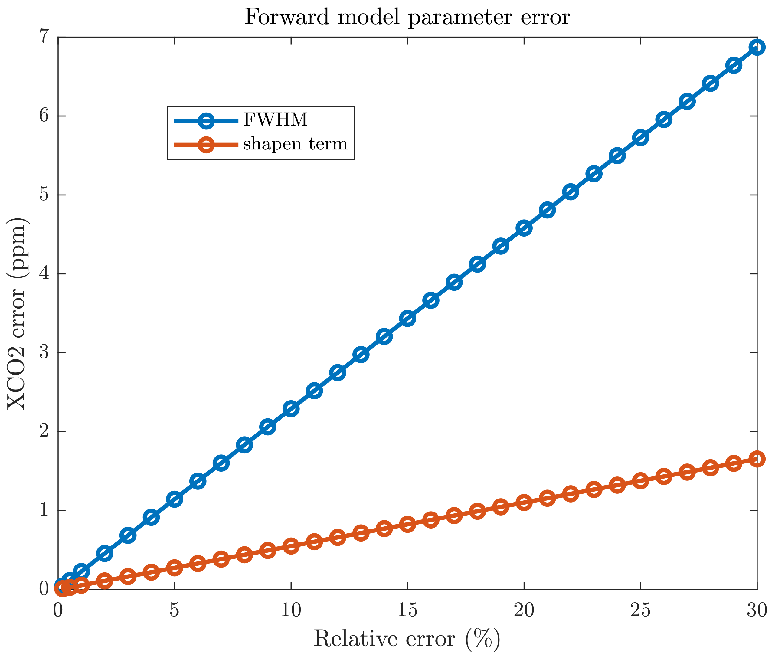
The additive wavelength-dependent zero-offset and Fourier-series correction in both the O2A and WCO2 bands are fitted in the TanSat XCO2 retrieval algorithm [10]. Both correction approaches considerably reduce the residual error in radiometric calibration and improve the fitting residual; they may also account for the effects of uncorrected stray light. However, the FWHM in the WCO2 band is several percentage points lower. The effect of error in FWHM on XCO2 retrieval still needs to be verified. We explored the retrieval impact of on-orbit ILS calibration error and uncertainties using a linear error analysis approach by including the ILS in the forward model. Synthetic TanSat spectra were modeled by a vector discrete ordinate radiative transfer model (VLIDORT) [23], with an interface optimized for TanSat. The XCO2 errors due to any of these ILS parameters can be readily calculated using the forward model parameter error. We focused on the FWHM and wing of ILS. Figure 11 shows the linear error analysis of the relative uncertainty of XCO2 due to the relative uncertainty in ILS width; the ILS is modeled by the stretch/sharpen function. To ensure the ILS-induced error is comparable to that of the XCO2 retrieval (1 ppm), the ILS width should be known to be within about 4%. The effect of wings is considerable when large uncertainty exists, as indicated by the forward model error induced by the sharpen term. For example, in Figure 9, the sharpen term in the WCO2 band varies from about 0.8 to 0.9. We obtain similar results using the super Gaussian+P7 function. However, the interference error due to ILS is negligible (not shown here) when the ILS width is retrieved as part of the state vector. Therefore, it is possible to constrain the ILS without jeopardizing XCO2 and account for the temporal variation in ILS as has been applied for OMI ozone profile retrieval [24]. However, ILS uncertainty may interact with other parameters beyond current error analysis, and ILS change is complicated (the shape may not be exactly the same as the ILS stretching and sharpening).
5. Conclusions
In this study, we characterized the on-orbit post-launch ILS for individual fitting windows, footprints, and bands of the TanSat instrument by fitting the measured solar spectrum with a high-resolution solar reference spectrum. We used different ILS functions to parameterize the ILS. Using the stretch/sharpen and super Gaussian+P7 functions remarkably improves the fitting residuals of the solar spectrum in both the O2A band and WCO2 bands. Using an asymmetric super Gaussian function does not improve the fitting residual compared with using the preflight ILS. Using a theoretical function could induce artificial temporal variation in the FWHM due to the spectral undersampling. The temporal variation in the derived on-orbit ILS functions shows considerable wavelength and footprint dependence. In the WCO2 band, the derived FHWMs are smaller than the preflight FWHM by up to −3.5%. We use the sharpen term and the P7 function to describe the ILS wings. The sharpen term was found to vary between 0.7 and 0.92, indicating uncorrected stray light depending on the wavelength, footprint and band. The derived ILS is sensitive to the stray light signals, and it should be well-characterized through on-ground calibration experiments.
The broadening of ILS wings in OCO-2 was demonstrated by the SIF signal [13]. TanSat behaves similarly to OCO-2 but derives larger-amplitude of the ILS wings. An ILS correction may also be needed to reduce the dependence of TanSat SIF retrieval on the offline bias correction. We estimated the effects of on-orbit changes in FWHM and amplitude of the tails on XCO2 retrieval by using a linear error analysis approach. A 4% uncertainty in the FWHM or a 20% uncertainty in the wings of the ILS can induce an error of up to 1 ppm in the XCO2 retrieval. However, differences in stray light between radiance and irradiance and scene heterogeneity may induce different errors in Earth-viewing radiance and solar irradiance. Future research is needed to implement the derived on-orbit ILS in the IAPCAS retrieval algorithm [10] and attempt to retrieve the ILS parameters simultaneously with XCO2, as the simulations show that the interference error in XCO2 due to simultaneous ILS fitting is negligible.
Future missions, such as TanSat-2, should account for the error in ILS. On-ground characterization of ILS shape and stray light is critical for greenhouse gas retrievals. Long-term in-flight monitoring of ILS shape is more useful [9] because the change in ILS shape cannot be represented by fitting theoretical functions when the number of solar lines is limited in the O2A, WCO2 and SCO2 bands. Increasing the spectral sample rate will also be helpful.
Author Contributions
Conceptualization: Z.C.; methodology: Z.C. and K.S.; formal analysis: Z.C.; draft: Z.C.; writing—review and editing: X.L., K.S., D.Y., C.L., and Y.L.; funding acquisition: Y.L. and Z.C.; SIF data analysis: L.Y. All authors have read and agreed to the published version of the manuscript.
Funding
This study was supported by the National Key R&D Program of China (grant no. 2019YFE0127500), Strategic Priority Research Program of the Chinese Academy of Science (grant no. XDA17010102), the National Natural Science Foundation of China (nos. 41875043 and 41905029), the Key Research Program of the Chinese Academy of Sciences (grant no. ZDRW-ZS-2019-1), and the Youth Innovation Promotion Association of CAS.
Data Availability Statement
The TanSat data used in the paper are publicly available at https://fy4.nsmc.org.cn/nsmc/en/satellite/TanSat.html (accessed on 10 March 2022).
Acknowledgments
We acknowledge Geoffrey Toon at JPL for providing solar line list data. We also thank Yanmeng Bi at CMA for the helpful discussion.
Conflicts of Interest
The authors declare no conflict of interest.
References
- Liu, Y.; Wang, J.; Yao, L.; Chen, X.; Cai, Z.; Yang, D.; Yin, Z.; Gu, S.; Tian, L.; Lu, N.; et al. The TanSat mission: Preliminary global observations. Sci. Bull. 2018, 63, 1200–1207. [Google Scholar] [CrossRef] [Green Version]
- Crisp, D.; Pollock, H.R.; Rosenberg, R.; Chapsky, L.; Lee, R.A.M.; Oyafuso, F.A.; Frankenberg, C.; O’Dell, C.W.; Bruegge, C.J.; Doran, G.B.; et al. The on-orbit performance of the Orbiting Carbon Observatory-2 (OCO-2) instrument and its radiometrically calibrated products. Atmos. Meas. Tech. 2017, 10, 59–81. [Google Scholar] [CrossRef] [Green Version]
- Cai, Z.; Liu, Y.; Yang, D. Analysis of XCO2 retrieval sensitivity using simulated Chinese Carbon Satellite (TanSat) measurements. Sci. China Earth Sci. 2014, 57, 1919–1928. [Google Scholar] [CrossRef]
- Chen, X.; Wang, J.; Liu, Y.; Xu, X.; Cai, Z.; Yang, D.; Yan, C.X.; Feng, L. Angular dependence of aerosol information content in CAPI/TanSat observation over land: Effect of polarization and synergy with A-train satellites. Remote Sens. Environ. 2017, 196, 163–177. [Google Scholar] [CrossRef]
- Yang, Z.; Zhen, Y.; Yin, Z.; Lin, C.; Bi, Y.; Liu, W.; Wang, Q.; Wang, L.; Gu, S.; Tian, L. Prelaunch radiometric calibration of the tan sat atmospheric carbon dioxide grating spectrometer. IEEE Trans. Geosci. Remote Sens. 2018, 56, 4225–4233. [Google Scholar] [CrossRef]
- Li, Z.; Lin, C.; Li, C.; Wang, L.; Ji, Z.; Xue, H.; Wei, Y.; Gong, C.; Gao, M.; Liu, L.; et al. Prelaunch spectral calibration of a carbon dioxide spectrometer. Meas. Sci. Technol. 2017, 28, 065801. [Google Scholar] [CrossRef]
- Hu, H.; Hasekamp, O.; Butz, A.; Galli, A.; Landgraf, J.; de Brugh, J.A.; Borsdorff, T.; Scheepmaker, R.; Aben, I. The operational methane retrieval algorithm for TROPOMI. Atmos. Meas. Tech. 2016, 9, 5423–5440. [Google Scholar] [CrossRef] [Green Version]
- Day, J.O.; O’Dell, C.W.; Pollock, R.; Bruegge, C.J.; Rider, D.; Crisp, D.; Miller, C.E. Preflight Spectral Calibration of the Orbiting Carbon Observatory. IEEE Trans. Geosci. Remote Sens. 2011, 49, 2793–2801. [Google Scholar] [CrossRef]
- van Hees, R.M.; Tol, P.J.J.; Cadot, S.; Krijger, M.; Persijn, S.T.; van Kempen, T.A.; Snel, R.; Aben, I.; Hoogeveen, R.W. Determination of the TROPOMI-SWIR instrument spectral response function. Atmos. Meas. Tech. 2018, 11, 3917–3933. [Google Scholar] [CrossRef] [Green Version]
- Yang, D.; Boesch, H.; Liu, Y.; Somkuti, P.; Cai, Z.; Chen, X.; Di Noia, A.; Lin, C.; Lu, N.; Lyu, D.; et al. Toward High Precision XCO2 Retrievals From TanSat Observations: Retrieval Improvement and Validation Against TCCON Measurements. J. Geophys. Res. Atmos. 2020, 125, e2020JD032794. [Google Scholar] [CrossRef]
- Wang, S.; van der A, R.J.; Piet, S.; Weihe, W.; Peng, Z.; Naimeng, L.; Fang, L. Carbon Dioxide Retrieval from TanSat Observations and Validation with TCCON Measurements. Remote Sens. 2020, 12, 2204. [Google Scholar] [CrossRef]
- Hong, X.; Zhang, P.; Bi, Y.; Liu, C.; Sun, Y.; Wang, W.; Chen, Z.; Hao, Y.; Zhang, C.; Tian, Y.; et al. Retrieval of Global Carbon Dioxide From TanSat Satellite and Comprehensive Validation With TCCON Measurements and Satellite Observations. IEEE Trans. Geosci. Remote Sens. 2021, 60, 1–16. [Google Scholar] [CrossRef]
- Sun, K.; Liu, X.; Nowlan, C.; Cai, Z.; Chance, K.; Frankenberg, C.; Lee, R.; Pollock, R.; Rosenberg, R.; Crisp, D. Characterization of the OCO-2 instrument line shape functions using on-orbit solar measurements. Atmos. Meas. Tech. 2017, 10, 939–953. [Google Scholar] [CrossRef] [Green Version]
- Liu, X.; Chance, K.; Kurosu, T.P. Improved ozone profile retrievals from GOME data with degradation correction in reflectance. Atmos. Chem. Phys. 2007, 7, 1575–1583. [Google Scholar] [CrossRef] [Green Version]
- Cai, Z.; Liu, Y.; Liu, X.; Chance, K.; Nowlan, C.; Lang, R.; Munro, R.; Suleiman, R. Characterization and correction of global ozone monitoring experiment 2 ultraviolet measurements and application to ozone profile retrievals. J. Geophys. Res. Atmos. 2012, 117, D07305. [Google Scholar] [CrossRef]
- Yao, L.; Yang, D.; Liu, Y.; Wang, J.; Liu, L.; Du, S.; Cai, Z.; Lu, N.; Lu, D.; Wang, M.; et al. A New Global Solar-induced Chlorophyll Fluorescence (SIF) Data Product from TanSat Measurements. Adv. Atmos. Sci. 2021, 38, 341–345. [Google Scholar] [CrossRef]
- Frankenberg, C.; Pollock, R.; Lee, R.A.M.; Rosenberg, R.; Blavier, J.F.; Crisp, D.; O’Dell, C.W.; Osterman, G.B.; Roehl, C.; Wennberg, P.O.; et al. The Orbiting Carbon Observatory (OCO-2): Spectrometer performance evaluation using pre-launch direct sun measurements. Atmos. Meas. Tech. 2015, 8, 301–313. [Google Scholar] [CrossRef] [Green Version]
- Toon, G.C. Solar line list for GGG2014, hosted by the carbon dioxide information analysis center. Inf. Anal. Cent. 2014. [Google Scholar] [CrossRef]
- Boesch, H.; Brown, L.; Castano, R.; Christi, M.; Crisp, D.; Eldering, A.; Fisher, B.; Frankenberg, C.; Gunson, M.; Granat, R.; et al. Orbiting Carbon Observatory (OCO)-2 Level 2 Full Physics Algorithm Theoretical Basis Document 2015. Available online: https://disc.gsfc.nasa.gov/OCO-2/documentation/oco-2-v6/OCO2_L2_ATBD.V6.pdf (accessed on 3 December 2015).
- Coddington, O.M.; Richard, E.C.; Harber, D.; Pilewskie, P.; Woods, T.N.; Chance, K.; Liu, X.; Sun, K. The TSIS-1 Hybrid Solar Reference Spectrum. Geophys. Res. Lett. 2021, 48, e2020GL091709. [Google Scholar] [CrossRef]
- Chance, K.; Kurosu, T.P.; Sioris, C.E. Undersampling correction for array detector-based satellite spectrometers. Appl. Opt. 2005, 44, 1296–1304. [Google Scholar] [CrossRef] [Green Version]
- Frankenberg, C.; Butz, A.; Toon, G. Disentangling chlorophyll fluorescence from atmospheric scattering effects in O2 A-band spectra of reflected sun-light. Geophys. Res. Lett. 2011, 38, L03801. [Google Scholar] [CrossRef]
- Spurr, R.J. VLIDORT: A linearized pseudo-spherical vector discrete ordinate radiative transfer code for forward model and retrieval studies in multilayer multiple scattering media. J. Quant. Spectrosc. Radiat. Transf. 2006, 102, 316–342. [Google Scholar] [CrossRef]
- Bak, J.; Liu, X.; Sun, K.; Chance, K.; Kim, J.H. Linearization of the effect of slit function changes for improving Ozone Monitoring Instrument ozone profile retrievals. Atmos. Meas. Tech. 2019, 12, 3777–3788. [Google Scholar] [CrossRef] [Green Version]
Figure 1.
TanSat mean solar spectrum at (a) O2A, (b) WCO2, and (c) SCO2 bands, and comparison with the reference solar spectra convolved with TanSat ILS. TanSat solar measurements were from footprint 4 on 1 March 2017.
Figure 1.
TanSat mean solar spectrum at (a) O2A, (b) WCO2, and (c) SCO2 bands, and comparison with the reference solar spectra convolved with TanSat ILS. TanSat solar measurements were from footprint 4 on 1 March 2017.

Figure 2.
Examples of tabulated preflight ILS of TanSat for the O2A band (pixel 620 in spectral direction, ∼768.6 nm), WCO2 band (pixel 240, ∼1608.8 nm), and SCO2 band (pixel 240, ∼2060.3 nm) (upper panel). The lower panel depicts the same but in log y scale. Nine footprints are shown in different colors.
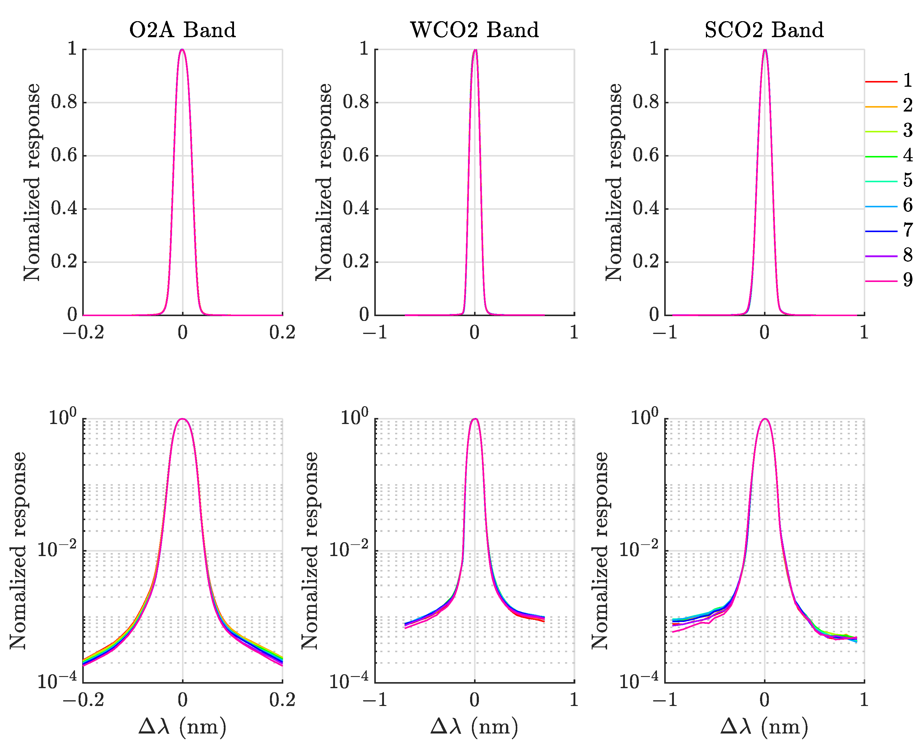
Figure 3.
(a) Preflight ILS, retrieved ILS using stretch/sharpen, super Gaussian+P7, and asymmetric super Gaussian function at 758 nm for footprint 1; (b) the same as for (a) but at 1596 nm and (c) at 2066 nm. FWHM () for each type of ILS function is shown.
Figure 3.
(a) Preflight ILS, retrieved ILS using stretch/sharpen, super Gaussian+P7, and asymmetric super Gaussian function at 758 nm for footprint 1; (b) the same as for (a) but at 1596 nm and (c) at 2066 nm. FWHM () for each type of ILS function is shown.
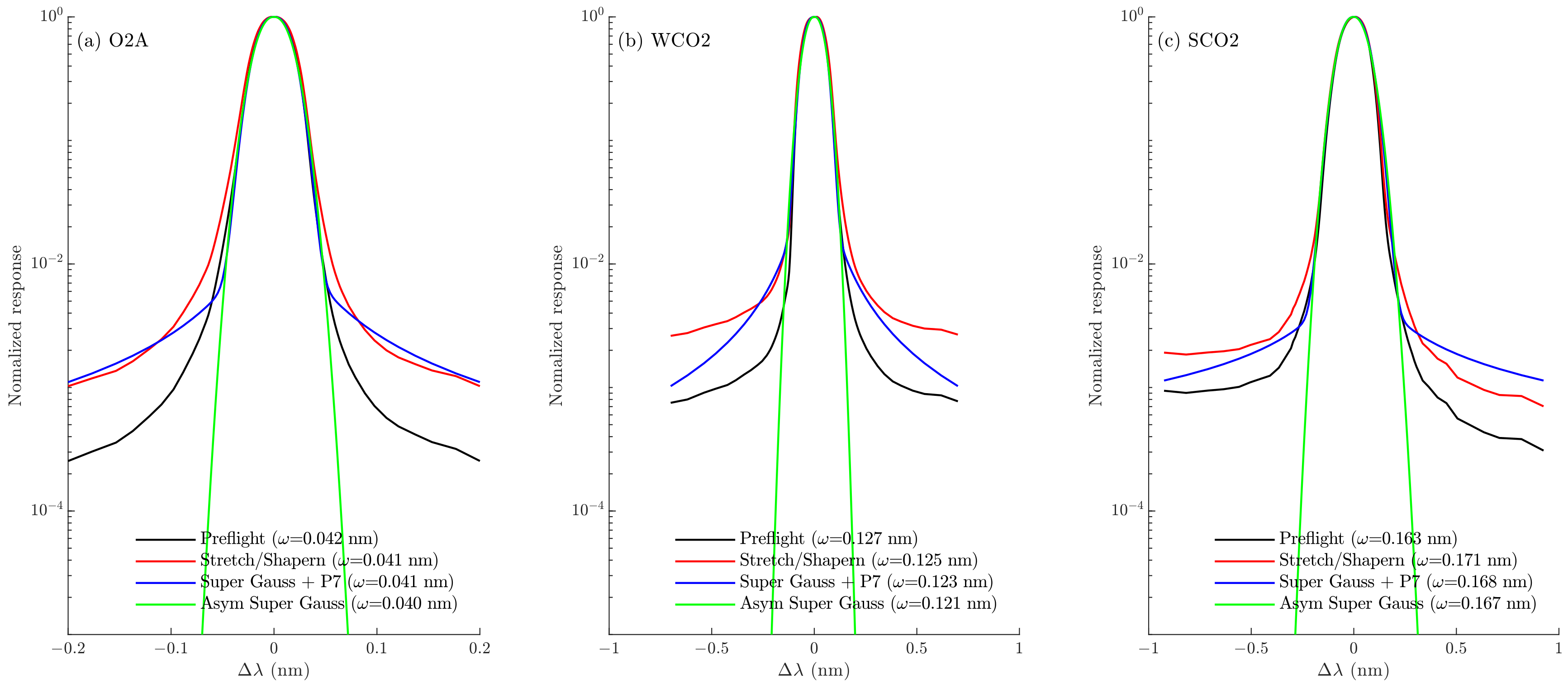
Figure 4.
(a–c) FWHM of retrieved ILS as a function of wavelength for three TanSat bands at footprint 1 on 1 March 2017. The black line denotes preflight ILS FWHM. (d–f) Average fitting residual of each fitting window using four different ILS functions. (g–i) Similar to (d–f) but for the fitting residual at each wavelength.
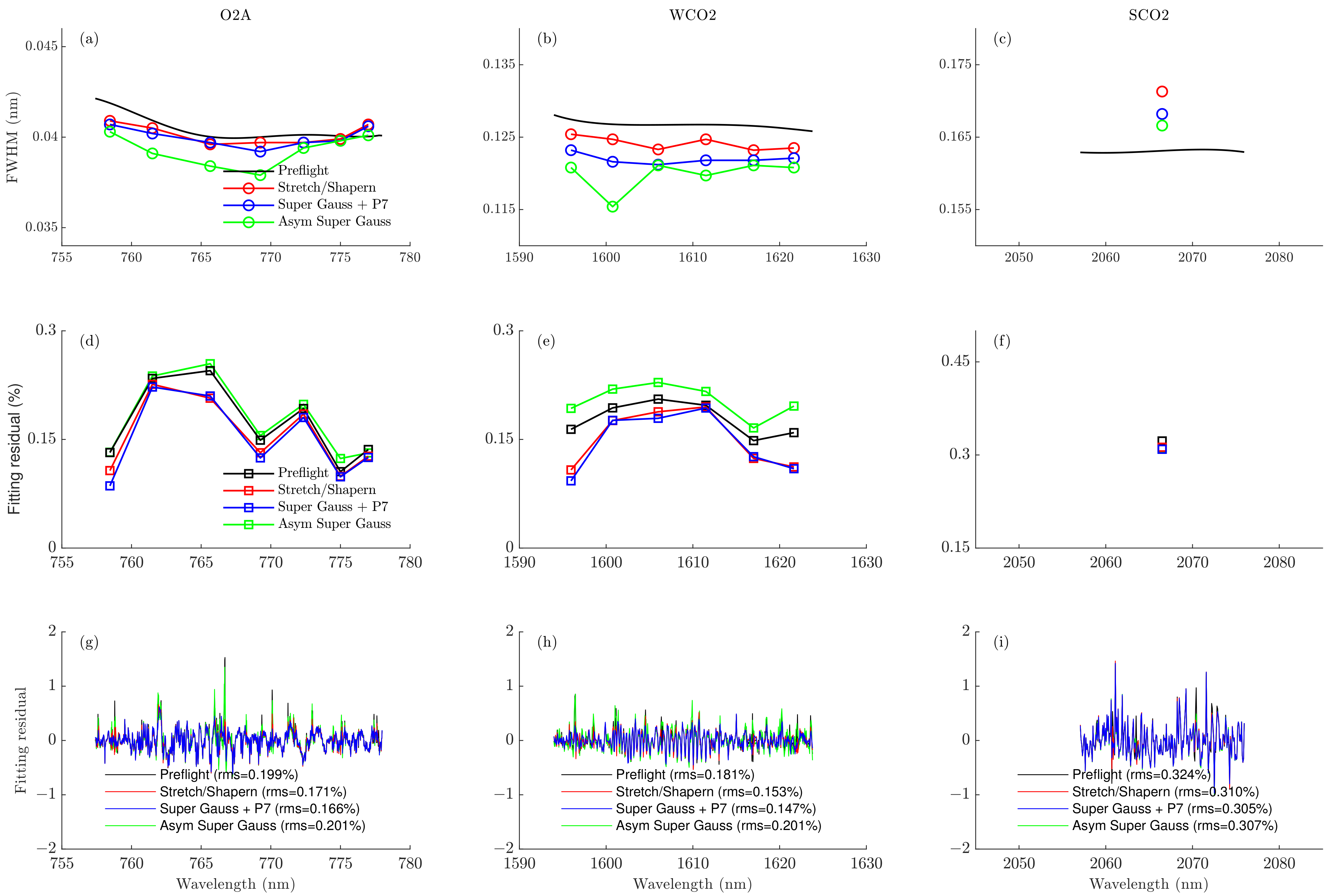
Figure 5.
(a) FWHM and (b) average fitting residual of retrieved ILS using four ILS functions for the O2A band at footprint 1 and fitting window 1 over time. (c,d) Similar to (a,b) but for fitting window 6, respectively.
Figure 5.
(a) FWHM and (b) average fitting residual of retrieved ILS using four ILS functions for the O2A band at footprint 1 and fitting window 1 over time. (c,d) Similar to (a,b) but for fitting window 6, respectively.

Figure 6.
(a) FWHM and (b) average fitting residual of retrieved ILS using four ILS functions for the WCO2 band at footprint 1 and fitting window 1 over time. (c,d) Similar to (a,b) but for fitting window 6, respectively.
Figure 6.
(a) FWHM and (b) average fitting residual of retrieved ILS using four ILS functions for the WCO2 band at footprint 1 and fitting window 1 over time. (c,d) Similar to (a,b) but for fitting window 6, respectively.

Figure 7.
Variation in relative difference between FWHM derived using stretch/sharpen function and preflight FWHM in fitting windows at the O2A band for all footprints. Dotted line represents 0%.
Figure 7.
Variation in relative difference between FWHM derived using stretch/sharpen function and preflight FWHM in fitting windows at the O2A band for all footprints. Dotted line represents 0%.
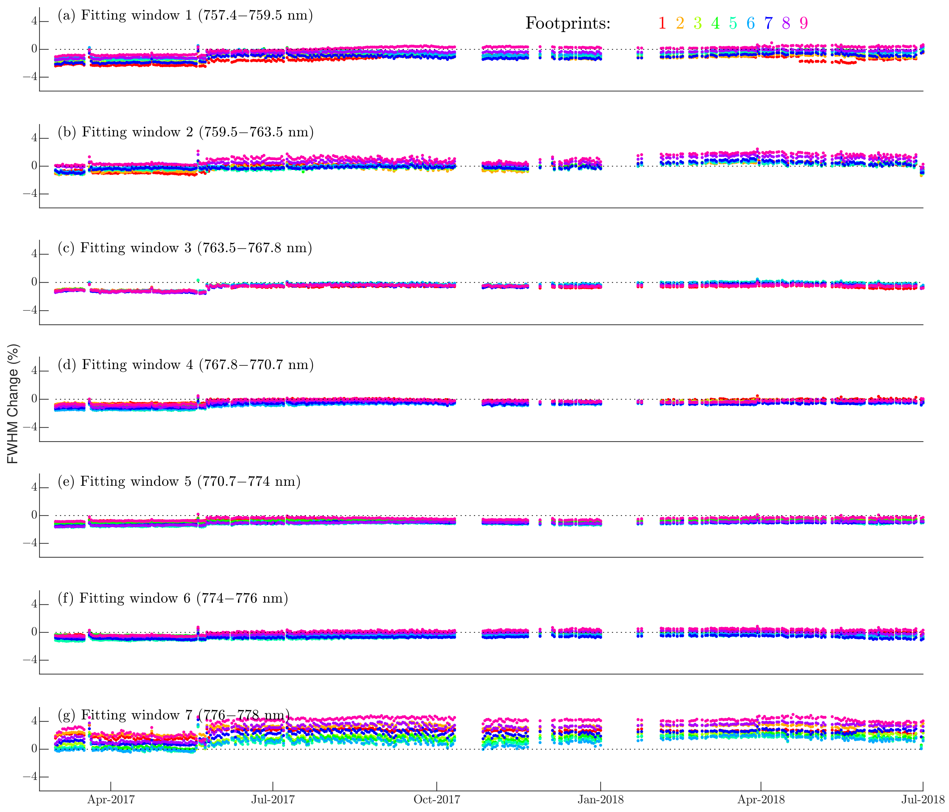
Figure 8.
Similar to Figure 7 but for 6 fitting windows at the WCO2 band.
Figure 8.
Similar to Figure 7 but for 6 fitting windows at the WCO2 band.
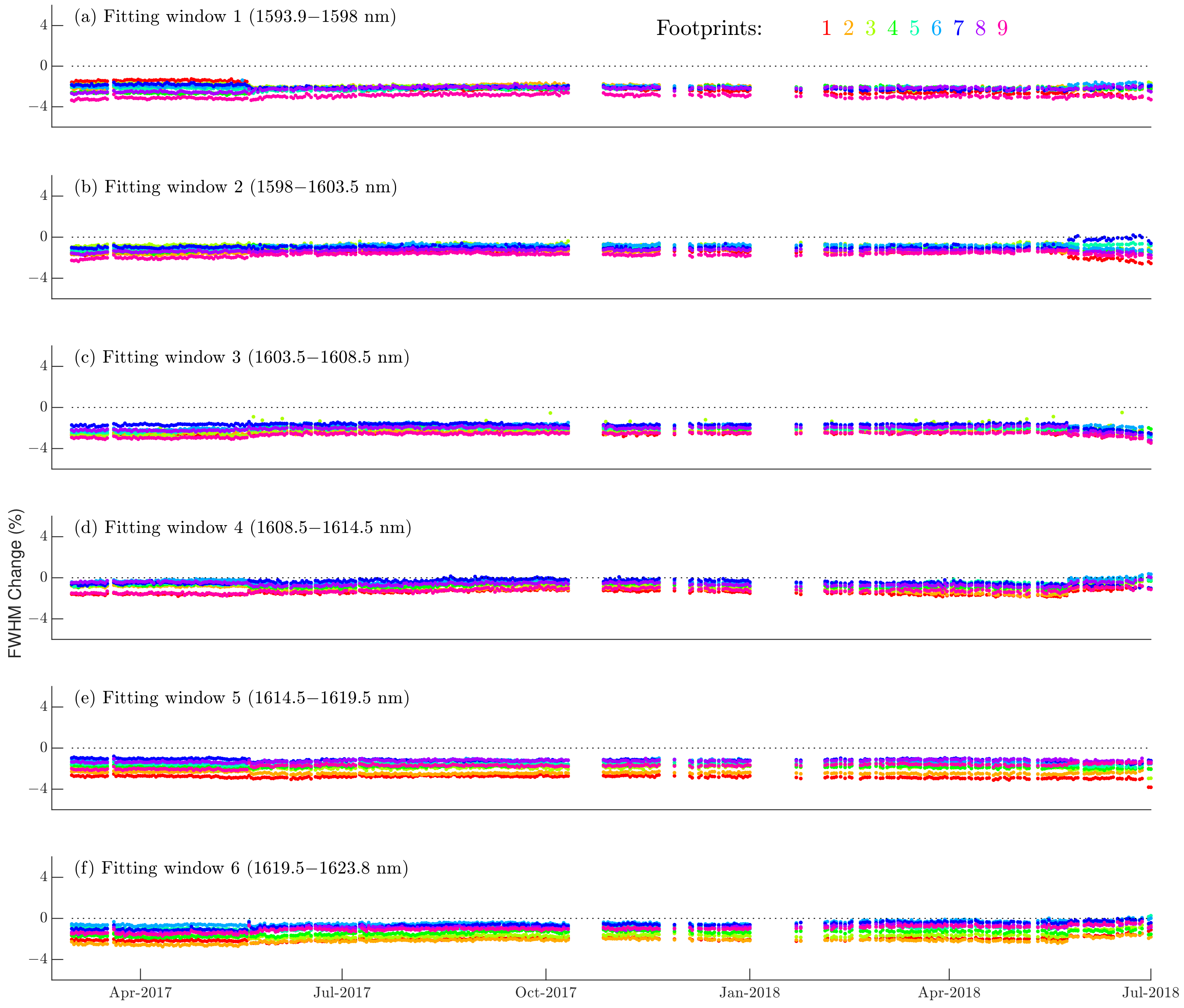
Figure 9.
Sharpen term over time for window 6 in the O2A band and window 5 in the WCO2 band.

Figure 10.
Time series of (a) SIF offset correction derived at 145 W msrm. Filling-in offset derived using (b) preflight ILS and (c) stretch/sharpen ILS.
Figure 10.
Time series of (a) SIF offset correction derived at 145 W msrm. Filling-in offset derived using (b) preflight ILS and (c) stretch/sharpen ILS.
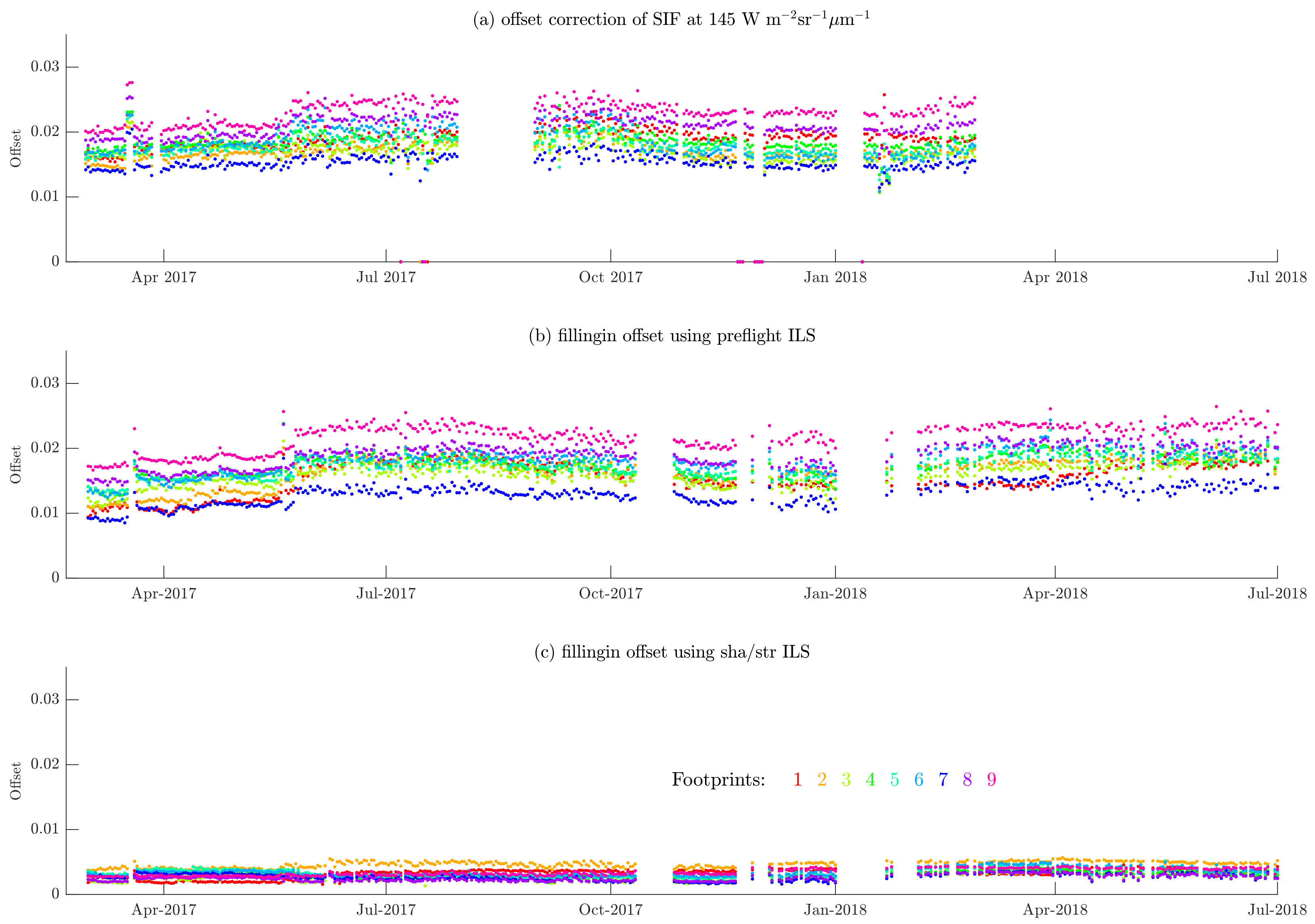
Figure 11.
Estimation of XCO2 retrieval error due to FWHM and sharpen term uncertainties using synthetic TanSat measurements. Reflectance was modeled with: surface albedo = 0.05, solar zenith angle = 30, and viewing zenith angle = 0.1.
Figure 11.
Estimation of XCO2 retrieval error due to FWHM and sharpen term uncertainties using synthetic TanSat measurements. Reflectance was modeled with: surface albedo = 0.05, solar zenith angle = 30, and viewing zenith angle = 0.1.
Publisher’s Note: MDPI stays neutral with regard to jurisdictional claims in published maps and institutional affiliations. |
© 2022 by the authors. Licensee MDPI, Basel, Switzerland. This article is an open access article distributed under the terms and conditions of the Creative Commons Attribution (CC BY) license (https://creativecommons.org/licenses/by/4.0/).
Share and Cite
MDPI and ACS Style
Cai, Z.; Sun, K.; Yang, D.; Liu, Y.; Yao, L.; Lin, C.; Liu, X. On-Orbit Characterization of TanSat Instrument Line Shape Using Observed Solar Spectra. Remote Sens. 2022, 14, 3334. https://doi.org/10.3390/rs14143334
AMA Style
Cai Z, Sun K, Yang D, Liu Y, Yao L, Lin C, Liu X. On-Orbit Characterization of TanSat Instrument Line Shape Using Observed Solar Spectra. Remote Sensing. 2022; 14(14):3334. https://doi.org/10.3390/rs14143334
Chicago/Turabian StyleCai, Zhaonan, Kang Sun, Dongxu Yang, Yi Liu, Lu Yao, Chao Lin, and Xiong Liu. 2022. "On-Orbit Characterization of TanSat Instrument Line Shape Using Observed Solar Spectra" Remote Sensing 14, no. 14: 3334. https://doi.org/10.3390/rs14143334
Note that from the first issue of 2016, this journal uses article numbers instead of page numbers. See further details here.