Bubble Plume Target Detection Method of Multibeam Water Column Images Based on Bags of Visual Word Features

Abstract

Bubble plumes, as main manifestations of seabed gas leakage, play an important role in the exploration of natural gas hydrate and other resources. Multibeam water column images have been widely used in detecting bubble plume targets in recent years because they can wholly record water column and seabed backscatter strengths. However, strong noises in multibeam water column images cause many issues in target detection, and traditional target detection methods are mainly used in optical images and are less efficient for noise-affected sonar images. To improve the detection accuracy of bubble plume targets in water column images, this study proposes a target detection method based on the bag of visual words (BOVW) features and support vector machine (SVM) classifier. First, the characteristics of bubble plume targets in water column images are analyzed, with the conclusion that the BOVW features can well express the gray scale, texture, and shape characteristics of bubble plumes. Second, the BOVW features are constructed following steps of point description extraction, description clustering, and feature encoding. Third, the quadratic SVM classifier is used for the recognition of target images. Finally, a procedure of bubble plume target detection in water column images is described. In the experiment using the measured data in the Strait of Georgia, the proposed method achieved 98.6% recognition accuracy of bubble plume targets in validation sets, and 91.7% correct detection rate of the targets in water column images. By comparison with other methods, the experimental results prove the validity and accuracy of the proposed method, and show potential applications of our method in the exploration and research on ocean resources.

1. Introduction

As one of the most widely used ocean survey equipment, multibeam sonars can acquire the full coverage of underwater topographic survey and simultaneously construct seabed backscatter strength images. In recent years, recording and processing the whole water column backscatter data using multibeam sonars have become possible, with the rapid improvement of computer processing power and storage capacity [1].

Multibeam water column images have been used to investigate marine biological resources (fish/fish school [2,3], krill [4], and seabed eelgrass [5,6]), study ocean physical changes such as internal waves [7,8], find underwater shipwrecks [9,10], and detect gas clouds [11] and bubble plumes [12,13,14,15] from seabed seeps. Innangi et al. [16] proposed a detection method of fish schools using multibeam water column images and obtained 3D shapes of various fish schools. Hughes Clarke et al. [9,17,18] studied the imaging principle, noise interference, and other basic knowledge of multibeam water column imaging, which laid a foundation for subsequent research. They also used water column image to estimate the minimum depth of a shipwreck (mast peak), which could provide a safety guarantee for shipping. Marques [19] used multibeam water column images to recognize and precisely locate spherical suspended targets and monitor seabed landslide activities. Gardner et al. [20] found a bubble plume with a depth of 1830 m and a height of 1400 m by using water column images collected from Kongsberg EM302 multibeam sonar in the coastal area of northern California. Weber et al. [21] discovered a bubble plume with 1100 m height using water column images from Kongsberg EM302 in the Gulf of Mexico. Various applications, especially in marine resource exploration and environment research of multibeam water column images have been proven by these studies.

Bubble plumes are the main manifestations of seabed gas leakage. The leaked gases could be the natural gas (methane), meaning the potential storage of natural gas hydrates. The gases also could be the mixed gases produced by decomposition of underwater dead plants and animals. Therefore, bubble plumes play important roles in the exploration of important resources (like natural gas hydrate) and the research of underwater environment [22,23,24,25]. How to accurately and efficiently recognize and detect bubble plumes in multibeam water column images is a hot research issue at present [26].

To recognize targets in sonar images, classifying the special target features has been proven as a feasible solution. Many studies have focused on detection and recognition of sonar image targets using classifiers of image features. Dobeck et al. [27] achieved automatic mine target detection and recognition in sonar images by using a k-nearest neighbor classifier of 45 extracted features, such as shape and intensity of mine targets. Tang et al. [28] studied the multi-channel texture classification algorithm by applying wavelet packet and Fourier transform on side-scan sonar images. The experimental results showed that the feature extraction method is vital for image classification. Reed et al. [29] achieved the recognition of sand slope targets in side-scan sonar images based on texture features, standard classifier, and Markov random field. Rhinelander et al. [30] combined feature extraction, edge filter, median filter, and support vector machine (SVM) classifier to achieve target detection and recognition in side-scan sonar images. Song et al. [31] studied the sonar image target segmentation method based on Markov random field and extreme learning machine. Wang [32] studied a target detection algorithm in side-scan sonar images using feature extraction method based on a neutrosophic set and diffusion maps. Moreover, a combination of various feature extraction methods (gray-level co-occurrence matrix, local binary pattern, Gabor, Tamura, multifractal spectrum, and others) and various classifiers (AdaBoost, back-propagation neural network, convolutional neural network, and others) have been applied on various targets in different sonar images.

In conclusion, numerous target feature extraction methods and classifiers have been used for target recognition and detection in sonar images. For various target recognition in different types of sonar images, the optimal features and classifiers are quite different. For the bubble plume target in multibeam water column, the optimal features and classifiers have yet to be studied. Zhao et al. [33] used Haar-like and local binary pattern feature and AdaBoost classifier to recognize the gas plume targets in multibeam water column images. This feature is suitable for vertical and strong-strength bubble plume targets, but recognition accuracy of inclined and weak-strength bubble plume target still needs to be improved.

In recent years, deep learning methods have been widely applied in recognition and detection of sonar image targets [34,35]. Deep learning methods usually need a large number of samples and labels to ensure model accuracy and generality. However, due to the particularity of sonar data collection and the difficulty in finding underwater targets, it is difficult to guarantee the sufficient number of sonar image target samples, which brings problems to the accuracy target recognition [36,37,38]. Another feasible solution is automatic sample augmentation using deep learning methods (like generative adversarial networks) in the case of small or even zero samples [39,40,41]. However, differences remain between the augmented and real samples, and the accuracy improvement of target recognition and detection using augmented samples still needs to be studied.

Therefore, in this article, we analyze the characteristics of bubble plume, select an applicable feature extraction algorithm and reasonable classifier, and finally realize the automatic accurate recognition and detection of bubble plume targets in multibeam water column images.

2. Theories and Methods

2.1. Basic Principle of Target Detection in Multibeam Water Column Images

The multibeam echo sounder system contains multiple sub-systems, including global navigation satellite system (GNSS), motion reference unit (MRU), gyro-magnetic compass, the bathymetric sonar and other auxiliary sensors [42,43]. Multibeam sonars emit sound waves through the projector arrays and then receive the backscatter strengths at multiple angles through the hydrophone arrays. By continuously recording the backscatter strengths from the transducer to the seabed and even under the seabed, we can obtain the observation of the whole water column, the seabed and surface sediments. The bubble plumes are some of the most important targets in the water column image because they could indicate the possible storage of natural gas hydrates or decomposition of underwater dead plants and animals. The bubble plumes usually were leaked from the seabed, rise to a certain height, and then dissipate. When the sound waves travel through these two different propagation medias (i.e., gas and water), the backscatter strengths from the bubbles are stronger than those from surrounding water, as shown in Figure 1.

In the multibeam water column images, the bubble plume targets are different from the background noises (Figure 1B). Some characteristics of the bubble plume targets in the water column images can be analyzed and concluded as follows:

• The bubble plume targets have much brighter grayscale features than the water column image background because the backscatter strengths from the gas bubbles are much stronger than those from the surrounding water;
• The bubble plume targets have special shape features. These targets are generally plume-like or ribbon-like shapes, which are obviously different from other water column targets (such as fish and fish school);
• The bubble plumes also have special orientation features. The bubble plumes usually range from the seabed to a certain height, and are usually approximately perpendicular to the seabed, but may be bent and oblique due to the ocean current effects. Due to side-lobe effects, bubble plumes in the minimum slant range are easier to detect;
• Special texture features exist around bubble plume targets. Due to the changes of two different propagation media, the texture features of the bubble plume and surrounding water are quite different.

These feature differences between the bubble plumes and background noises are the basis for the target recognition and detection method in a multibeam water column image.

As analyzed, the bubble plume targets have special grayscale, shape, orientation, and texture features. In the following sections, the bag of visual words (BOVW) features of bubble plume targets are extracted and used to represent these features, and the SVM classifier is used for binary classification of the BOVM features. Then, the recognition and detection procedures of bubble plume targets in the water column image are introduced in detail.

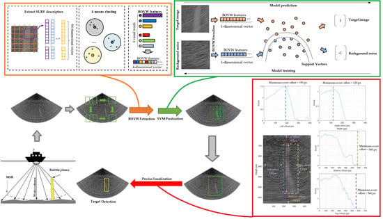
2.2. BOVW Features of Multibeam Water Column Images

The BOVW features were originally used for text classification by calculating the frequencies of important words in the text. The BOVW feature applies the same idea into image classification [44]. The images do not contain any concrete words; therefore, visual vocabulary needs to be constructed using feature point extraction methods, such as speeded up robust features (SURF) (Figure 2B), then the visual vocabulary is established by clustering these SURF descriptors (Figure 2C), and finally, the BOVW features can be encoded by calculating the frequencies of each visual words in the visual vocabulary (Figure 2D). These steps are shown in Figure 2 as:

• Step 1. All the SURF descriptors (64-dimensional eigenvectors) of interest points from sample images are extracted by SURF detection or uniform-grid-point selection;
• Step 2. Due to the excessive number SURFs extracted, the SURFs of all sample images were clustered using k-means to obtain k category;
• Step 3. For any image, the SURF points can be extracted using the interest point selection (Step 1) and calculated as 64-dimensional eigenvectors, then these SURF descriptions are classified into each category (Step 3);
• Step 4. The occurrence frequencies of all the SURF clustering categories are calculated to form the k-dimensional BOVW feature vector.

2.2.1. SURF Descriptors Extraction

The visual vocabulary of BOVW features need to be constructed by clustering the extracted point features from all different categories of sample images. SURF, as a scale invariant feature, can be used as both detectors and descriptors of interest points at any scale [45]. In multibeam water column image, SURF is also suitable for the detection and description of bubble plume target feature points [46].

The SURF method uses the Hessian matrix $H\left(\mathit{p},\sigma \right)$ to detect and describe the interest points p(x, y) at scale σ as

$$H\left(\mathit{p},\sigma \right)=\left[\begin{array}{cc}{L}_{xx}\left(\mathit{p},\sigma \right)& L_{xy}\left(\mathit{p},\sigma \right)\\ L_{yx}\left(\mathit{p},\sigma \right)& L_{yy}\left(\mathit{p},\sigma \right)\end{array}\right],$$

(1)

where L is the convolution of the Gaussian second-order derivative with the image.

As shown in Figure 3, detected SURF points from the target images and background noises are significantly different in feature scale, orientation and distribution, which proves the effectiveness of SURF points as the visual words of water column images. However, affected by different kinds of noises, detected SURF points from different water column images could vary greatly under the same Hessian threshold. If SURF detection is used to find interest points, some features of the target and background images could be ignored. Therefore, we use the uniform-grid-point selection to ensure that all the features in the target and background image can be extracted (Figure 2B).

The SURF descriptors are used to describe the uniform-grid selected points in the water column images. Before feature description, the main orientation of the descriptor is set as upright because no rotation is applied in the water column images. The steps for extracting SURF descriptors are listed as follows:

• Select the regions around key points and divide them into 4 × 4 small regions;
• Calculate Four features (dx, dy, |dx| and |dy|) of the sampling point corresponding to the Haar response in each small region;
• Construct and normalize the 64-dimensional (4 × 4 × 4) eigenvector of each key point.

Therefore, all the SURF descriptors of the uniform-grid selected points in the image can be described using the normalized 64-dimensional eigenvectors (Figure 2B). The grid size would determine the number of extracted points, which would be discussed in the experimental section.

2.2.2. Clustering SURF Descriptors

The visual vocabulary of water column images is constructed based on SURF descriptors of uniform-grid selected points. For sample sets containing many images, all of the SURF descriptors (i.e., the 64-dimensional eigenvector) of each image need to be extracted and summarized to obtain the special BOVW features that can describe the bubble plume targets. Moreover, these extracted SURF descriptors need to be clustered to limit the BOVW feature dimension. k-means, as an efficient clustering method, is suitable for clustering these SURF descriptors. The steps are the following:

• The k-mean++ algorithm is used to initialize k centroids c(j) (j = 1, …, k);
• The Euclidean distance L_j between each SURF 64-dimensional eigenvector v and the centroids c(j) is calculated as

$$L_j=\sqrt{{\displaystyle \sum }_{i=1}^{64}{\left(v_i-c{\left(j\right)}_i\right)}^2},j=1,\dots ,k.$$

(2)

3.

Each eigenvector is assigned to the nearest centroid and the k centroids are recalculated;

4.

Steps 2 and 3 are repeated until all the cluster assignments are stable (Figure 4B).

The clustering number k determines the visual vocabulary number and the dimension of BOVW features. Considering the noises affecting water column images, an extremely small visual vocabulary number will lead to the confusion of different features, and an extremely large visual vocabulary number will cause a huge waste of calculation resources. Therefore, determining k is important and would affect the final recognition accuracy, which would be discussed in the experimental section.

2.2.3. Image Coding Using BOVW Feature

In the previous section, a k-size visual vocabulary is obtained by clustering all the visual words (SURF eigenvectors). For a single image, the BOVW feature is the k-size vector by counting the occurrence frequencies of all the visual words in the vocabulary. The histograms of visual words are shown in Figure 5.

To make BOVW features suitable for following target recognition and detection, the BOVW feature [x₁, x₂, … x_i, …, x_k] needs to be normalized using L₂ normalization, as

$${\mathit{y}}_i=\frac{{\mathit{x}}_i}{\sqrt{{\sum }_{i=1}^k{\mathit{x}}_i^2}},$$

(3)

where y is the corresponding normalized vector and k is the vocabulary size.

The SURF descriptors extracted from bubble plume targets and background noise image are obviously different in scales and orientations (Figure 3); therefore, BOVW features as bags of these SURF descriptors can effectively represent grayscale, shape, orientation, and texture features of bubble plume targets. In the following sections, BOVW features are used for target recognition and detection.

2.3. Bubble Plume Recognition Using Support Vector Machine

Based on the SURF descriptor differences between bubble plume target and background noise images, the recognition of bubble plume targets can be done by classification of the BOVW features. Taking the target images as positive samples and the background images as negative samples, recognition becomes binary classification. In this section, a SVM classifier is used to binarily classify the BOVW features of bubble plumb target and background noise image. The overall procedure is shown as Figure 6.

2.3.1. Support Vector Machine

As a kernelized method, selection of kernel functions seriously affects the classification accuracy of the SVM classifier. To process the extracted BOVW features (k-dimensional eigenvectors), our work uses the nonlinear SVM classifier using the quadratic polynomial kernel. For any eigenvectors x_i and x_j, the quadratic polynomial kernel function κ is:

$$\kappa \left({\mathit{x}}_i,{\mathit{x}}_j\right)={({\mathit{x}}_i^T{\mathit{x}}_j)}^2.$$

(4)

Based on the SVM dual problem, SVM classification of the BOVW eigenvectors consists of the following steps:

• Selection of the quadratic polynomial kernel function, where the SVM problem could be converted to the convex quadratic programming problem as follows:

$$\begin{gathered} \underset{\alpha }{\mathit{\text{max}}}{\displaystyle \sum }_{i=1}^m{\alpha }_i-\frac{1}{2}{\displaystyle \sum }_{i=1}^m{\displaystyle \sum }_{j=1}^m{\alpha }_i{\alpha }_j{y}_i{y}_j{({\mathit{x}}_i^T{\mathit{x}}_j)}^2 \\ \text{subject to }{\displaystyle \sum }_{i=1}^m{\alpha }_i{y}_i=0,{\alpha }_i\ge 0,i=1,2,\dots ,m. \end{gathered}$$

(5)

2.

Based on the sequential minimal optimization (SMO) algorithm, the optimal solution is

$${\mathit{\alpha }}^{*}={\left({\alpha }_1^{*},{\alpha }_2^{*},\dots ,{\alpha }_N^{*}\right)}^T$$

(6)

3.

Selection of α_j^* as one component of α^*, satisfying 0 < α_j^* < C (C is the hyperparameter, called box constraint, to avoid overfitting). Then, we calculate

$${\mathit{b}}^{*}=y_j-{\displaystyle \sum }_{i=1}^m{\alpha }_i{y}_i{({\mathit{x}}_i^T{\mathit{x}}_j)}^2.$$

(7)

4.

The kernel function is used to replace the inner product, and the quadratic SVM becomes

$$f\left(\mathit{x}\right)={\displaystyle \sum }_{i=1}^N{\alpha }_i^{*}{y}_i{({\mathit{x}}_i^T{\mathit{x}}_j)}^2+{\mathit{b}}^{*}.$$

(8)

The hyperparameter box constraint and feature scale also affect the SVM classification accuracy and need to be updated during SVM training.

After training, the SVM can be used for prediction of input images. The binary loss is a function of the class label and classification score that determines how well a binary learner classifies an image into the class. The prediction score P is calculated using Hinge binary learner loss function which provides a negated average binary loss in a domain as (–∞, ∞).

$$P=\frac{\mathit{\text{max}}\left(\begin{array}{ll}0,& 1-y_{j}f\left(j\right)\end{array}\right)}{2},$$

(9)

where, y_j is a class label for the SVM binary classifier in the set (–1,1), and f(j) is the model score for input image j.

2.3.2. Recognition Procedure of Bubble Plume Targets

To recognize the bubble plume targets in the water column images, we carefully establish the positive and negative sample sets, construct the visual vocabulary based on clustering SURF points, and encode BOVW features of each sample image. Then, the SVM binary classifier is trained and used to recognize the target sample images. The flow diagram of bubble plume target recognition is shown in Figure 7. Only training image samples are used in establishing the visual vocabulary.

2.3.3. Recognition Accuracy Assessment

The prediction results of the target recognition model only contain two results, namely, the bubble plume target images or background noise images; therefore, the confusion matrix can be used to describe model accuracy for binary classification, as shown in

Table 1. Confusion matrix of binary classification.

Truth	Predicting Results
	True	False
Positive	True Positive (TP)	False Positive (FP)
Negative	True Negative (TN)	False Negative (FN)

TP and FP indicate that positive samples are identified as positive and negative samples, respectively, while TN and FN indicate that negative samples are identified as negative and positive samples, respectively.

. The accuracy assessments using the confusion matrix are listed in

Table 2. Accuracy assessment of SVM binary classification.

Accuracy Assessment	Computational Formula
Accuracy	$A=\frac{TP+TN}{TP+FP+TN+FN}$	(10)
Precision ratio	$P=\frac{TP}{TP+FP}$	(11)
Recall ratio	$R=\frac{TP}{TP+FN}$	(12)
Harmonic mean	$F_1=\frac{2TP}{2TP+FP+FN}$	(13)

.

2.4. Target Detection Using BOVW Features

2.4.1. Precise Target Localization

Based on the recognition method, the flow diagram of bubble plume target detection is shown as Figure 8.

A moving search window (Figure 8b) is used to traverse the water column image (Figure 8a), and the score of each window image is predicted by the recognition model based on the BOVW feature and SVM classifier. The size of the moving search window is close to the sample image size, and the moving step was set as 1/4 of the search window size. After traverse, the bubble target is covered by many search windows (Figure 8c), and the outline rectangle of these detection windows can be extracted (as the green boundary in Figure 8d). The initial detection of the bubble plume target is obtained, and more precise detection results (Figure 8g) are processed by precise localization (Figure 8d–f).

The precise localization method is intended to achieve more accurate detection boundary by gradually shortening the boundary range of the detection frame to obtain higher model prediction scores. The steps are as follows:

• First, gradually shrink the left boundary to the right, calculate the prediction scores of the reduced images, and select the maximum-score position as the final left boundary;
• Second, gradually shrink the right boundary to the left, calculate the scores of the reduced images, and select the maximum-score position as the final right boundary as the red boundary in Figure 8e;
• Third, based on the above detection boundary, gradually shrink the top boundary to the bottom, calculate the scores of the reduced images, and select the zero-score position as the final bottom boundary;
• Finally, gradually shrink the bottom boundary to the top, calculate the scores of the reduced images, and select the zero-score position as the final top boundary as the yellow boundary in Figure 8f.

According to the shape and orientation characteristics of the bubble plume target, the prediction score gradually increases as the initial detected left/right boundary shrinks to the right/left, but gradually decreases when the target begins to get lost in the image (after the maximum score). As to the top and bottom boundaries, the prediction score does not change significantly when the image shrinks in the top-bottom direction. However, when the image shrinks exceeding the bottom/top boundary and does not contain any targets, the score rapidly decreases to the zero value.

For the multiple-target case, independent detection areas can be distinguished and obtained based on the connectivity of detection frames. In each independent detection area, accurate detection of these targets can be achieved using the aforementioned method.

2.4.2. Detection Accuracy

Intersection over Union (IoU) is a common standard for measuring the detection accuracy of image targets. IoU measures the correlation between ground truth and predicted bounding boxes. Higher correlation means higher detection accuracy.

For ground-truth box as A and predicted box as B, the IoU of A and B can be calculated as

$$IoU=\frac{A\cap B}{A\cup B}.$$

(14)

Taking 0.5 as the IoU threshold, the correct detection can be defined as

$$\mathit{\text{Correct}}=\left\{\begin{array}{cc}\mathit{\text{true}},& IoU\ge 0.5\\ \mathit{\text{false}},& IoU<0.5\end{array}\right..$$

(15)

The correct detection rate is calculated using the correct detected target number N_c divided by the total target number N:

$${\mathit{\text{rate}}}_c=\frac{N_c}{N}.$$

(16)

3. Experiments and Results

To verify the validity and performance of the proposed method in this study, the measured multibeam water column data in the Strait of Georgia in 2012 were used for bubble target recognition and detection in the experiment, as shown in Figure 9. The multibeam sonar used was Kongsberg EM 710 with an operating frequency of 73–81 kHz, across-track beam aperture of approximately 130° and fixed beam number of 128 was recorded in the measurement. In the experiment, our method was implemented using MATLAB codes and built-in functions, as explained in Appendix A. The experiment consists of two parts:

• BOVW feature extraction and training and validation of SVM classifier. During data preparation, the measured multibeam data were used to construct the water column images. The images containing bubble plume target and only background noises were extracted as positive and negative samples and distributed in the training and validation sample sets. Then, the BOVW features were extracted from these images and the SVM classifier was trained using these features;
• Bubble target detection in water column images. Based on the recognition model using BOVW and SVM, the precise detection method of bubble plume targets was applied to detect all of the bubble plume targets in the water column images of the EM 710 multibeam sonar to prove the validity and generality of our detection method.

3.1. BOVW Feature Extraction and Classification

In this experiment, the recorded multibeam water column data (in *.wcd and *.all file) were decoded based on EM data format. Then, the water column images were constructed using the water column data packets.

3.1.1. Sampling from Multibeam Water Column Images

Positive samples which contain the bubble plume targets, and negative samples which contains only background noises, are manually extracted and labeled to establish the sample set, as shown in Figure 10. To avoid the problem of sample imbalance, the numbers of positive and negative samples are the same as 700. The size of each sample image was unified as 256 × 256 pixels.

The positive samples included partial or whole bubble plume targets in water column images. These positive samples were identified and labeled manually. The negative samples contained various noise background images and some other targets (like fishes) which were not discussed in this study. Meanwhile, because the water column images are fan-shaped, the edge parts of the fan-shaped images were also considered in the positive and negative samples to avoid the impact of edge SURF points on visual vocabulary construction.

3.1.2. Visual Vocabulary Construction and BOVW Feature Encoding

The visual vocabulary is the basis for encoding BOVW features. To construct the visual vocabulary, the total sample set was divided into the training and validation set in a ratio of 7:3. The visual vocabulary was constructed based on the image data of the training set to achieve the BOVW feature encoding of both the training and validation sets.

The SURF point descriptions of all the images in the training set need to be extracted according to the reasonable selection method, and then all SURF points were clustered to construct the visual vocabulary. Considering the sample image size as 256 × 256 px, several different SURF point extraction methods using 8 × 8, 16 × 16, 32 × 32 grids and SURF detector with different vocabulary word number k were selected and compared in the experiment, respectively, and the corresponding results were listed and shown in

Table 3. Parameter selection in constructing visual vocabulary.

SURF Point Extraction Method	Word Number of Visual Vocabulary	SURF Point Number	Strongest PointNumber	Point Number for Each Category	Training Accuracy	Validation Accuracy
Grid [8 × 8]	200	4,014,080	3,211,060	1,605,530	0.62	0.60
	300				0.84	0.83
	400				0.86	0.83
	500				0.71	0.69
Grid [16 × 16]	200	1,003,584	802,816	401,408	0.74	0.73
	300				0.81	0.76
	400				0.74	0.72
	500				0.79	0.77
Grid [32 × 32]	100	250,880	200,704	100,352	1.00	0.90
	200				1.00	0.93
	300				1.00	0.95
	400				1.00	0.94
	500				1.00	0.94
Detector	200	419,928	331,000	165,500	0.86	0.79
	300				0.47	0.46
	400				0.96	0.89
	500				0.92	0.80

The training and validation accuracy were calculated using the same SVM classifier.

.

The training and validation accuracy of each SURF point extraction method using the quadratic SVM classifier were calculated, and the validation accuracies were sorted out as Figure 11.

Table 3 shows that different SURF point extraction methods have significant effects on the accuracy of the recognition model. In the grid extraction methods, with the increase in the grid size, the number of extracted SURF points gradually decreased, but the model accuracies may increase or decrease, indicating the particular importance of that reasonable feature scale. The detector method discovered feature points through the SURF detection algorithm. When the vocabulary word number was set as 300, the training and validation accuracies were both less than 0.5, which showed the difficulty of finding enough feature points in noise-affected sonar images by SURF algorithm.

By comparison, the grid selection method using 32 × 32 px grids was used in the experiments, and the vocabulary word number k was set as 300.

3.1.3. SVM Classifier Training and Validation

To train an SVM classifier, the kernel function needs to be specified first. Different classifiers were used to classify the BOVW features obtained in Section 3.1.2, and the validation accuracy, training time, and prediction speed of each classifier were computed and listed in

Table 4. Comparison of different classifiers using BOVW features.

Classifier	Validation Accuracy (%)	Prediction Speed (Observation/s)	Training Time (s)
Medium Tree	90.3	750	8.15
Linear Discriminant	92.5	850	10.36
Logistic Regression	72.1	550	20.63
Linear SVM	98.3	860	10.16
Quadratic SVM	98.6	810	10.01
Cubic SVM	98.4	800	10.56
Medium Gaussian SVM	97.9	1200	11.07
Medium KNN	95.2	950	12.61
Bagged Trees Ensemble	96.9	600	19.65

. By comparison, the quadratic SVM classifier had the highest validation accuracy, reasonable training time, and prediction speed. Therefore, the quadratic function was chosen as the SVM kernel function.

After determining the kernel function, the hyperparameters, including the box constraint and feature scale, also need to be optimized. The hyperparameter box constraint (also called soft margin) controls the maximum imposed penalty of observed values that violate the margins to prevent model overfitting. If the box constraint is larger, the SVM classifier allocates fewer support vectors, resulting in longer training times.

SVM classifiers are also sensitive to the feature scales. The hyperparameter Feature Scale is used to scale the feature parameters, which means that all the elements of the BOVW features should be divided by the Feature Scale value. During the training process, the hyperparameters of the SVM classifier were optimized by finding the minimum model validation loss when constantly changing the Box Constraint and Feature Scale hyperparameter values, as shown in Figure 12.

After training, the SVM model was used to predict the image data, and the results of some water column images were listed in

Table 5. Prediction results of water column images set using BOVW features.

	Test Image	BOVW Feature	Prediction Score	Prediction Class	Manual Label
(a)			(0, −2.8254)	Bubble plume	Bubble plume
(b)			(0, −1.4815)	Bubble plume	Bubble plume
(c)			(0, −2.6271)	Bubble plume	Bubble plume
(d)			(0, −1.2373)	Bubble plume	Bubble plume
(e)			(−1.4502, 0)	Noise	Noise
(f)			(−1.3467, 0)	Noise	Noise
(g)			(−1.2134, −0)	Noise	Noise
(h)			(−0.9665, −0.0335)	Noise	Noise
	Overall	Confusion Matrix	$\left[\begin{array}{cc}0.95& 0.05\\ 0.00& 1.00\end{array}\right]$	Validation Accuracy	0.98

. As shown in the table, these images which contained bubble plume targets (Table 5a–d) had more valid SURF points and more abundant visual words. Noise background images (Table 5f–g) usually had fewer valid SURF points and the corresponding visual words were relatively simple.

For images in Table 5c,e, the noise backgrounds were quite similar, so the BOVW features of these two images were also similar to each other. However, obvious differences existed in the frequencies of special visual words (i.e., near index 190) between these two images, which proved the validity of the BOVW features in the recognition of the bubble plume targets. By calculation, the prediction accuracies of the training and validation set were 0.99 and 0.98, respectively.

3.2. Automatic Detection of Bubble Plume Target in Water Column Image

After verifying BOVW features and SVM classifier in recognition of bubble plume targets, we carried out the target detection experiment of water column images based on the proposed procedure (Figure 8).

Fixed and floating anchors are typically used in the detection of the possible targets to find the initial positions, as shown in Figure 13. The usage of fixed anchors (Figure 13a) may result in missing detection of small targets or losing parts of large targets. The usage of floating anchors can effectively avoid these problems, but may result in large initial detection boxes (Figure 13c). Therefore, further precise target localization is needed, as shown in Figure 14.

As shown in Figure 14c,e, the prediction score of the image gradually increased by constantly narrowing the detection box in the left/right directions. When the target boundary was reached, the score reached the maximum value, then started to decrease. When the detection box reached the other boundary of the target, the score would be close to zero because the image contained only background noises. Thus, the position of the maximum prediction score indicated the left and right boundary of the target detection box. Moreover, the maximum-score position in the left/right direction should correspond to the zero-score position in the right/left direction.

After determining the left and right boundaries, the top and bottom boundaries could be further obtained. Due to the orientation of the bubble plume target, the top/bottom boundaries could not be determined by the minimum value of the score curves, as shown in Figure 14b,f. Thus, the position of the top/bottom boundary should be determined by the minimum value of the bottom/top score curves. The final detection box is shown in Figure 14d, with prediction score 3.49 much larger than the initial score 0.88.

More water column images from the experimental data were processed by our detection method, and the detection results were obtained in Figure 15. As shown in Figure 15, the bubble plume targets of different sizes and backscatter strengths had been correctly detected. Taking the IoU value not less than 0.5 as the correct results, we calculated the correct detection rate of bubble plume targets in all the testing water column images as 91.7%. Therefore, the experimental results prove the validity and correctness of our detection method.

4. Discussion

In this section, our recognition and detection method of bubble plume targets in water column images was compared with other methods.

4.1. Feature and Classifier Comparison

To compare with the proposed method, various combinations of feature extraction methods and classifiers were used for the recognition of bubble plume targets in the water column images. These extracted features included gray-level cooccurrence matrix (GLCM), Tamura, local binary pattern (LBP), histogram of oriented gradient (HOG), the combination of these features, and Haar-LBP [33]. The results are shown in

Table 6. Comparison validation accuracies of various feature extraction and classifier.

Feature Extraction Method	Feature Number	Classifier	Accuracy (%)	Precision Ratio (%)	Recall Ratio (%)	F1 (%)
GLCM (d = 1)	12	Linear SVM	77.59	75.32	82.07	78.55
GLCM (d = 5)	12	Medium Tree	71.03	67.84	80.00	73.42
GLCM (d = 10)	12	Cosine KNN	70.69	67.65	79.31	73.02
GLCM (d = 1&5)	24	Logistic Regression	82.41	81.76	83.45	82.59
Tamura	3	Medium Tree	79.31	81.48	75.86	78.57
Tamura	6	Fine Tree	84.48	84.25	84.83	84.54
LBP (64 × 64)	59	Medium Gaussian SVM	90.00	94.62	84.82	89.45
LBP (64 × 64)	10	Medium Gaussian SVM	79.31	78.15	81.38	79.73
LBP (32 × 32)	236	Cubic SVM	94.14	94.44	93.79	94.12
HOG (32 × 32)	36	Weighted KNN	82.76	82.31	83.45	82.88
HOG (16 × 16)	324	Quadratic SVM	89.66	89.66	89.65	89.65
HOG (8 × 8)	1764	Linear SVM	76.55	74.21	81.38	77.63
GLCM + Tamura	30	Quadratic SVM	91.72	90.60	93.10	91.84
GLCM + LBP	83	Quadratic SVM	91.38	90.54	92.41	91.47
GLCM + HOG	60	Quadratic SVM	90.34	87.74	93.79	90.67
Tamura + LBP	65	Quadratic SVM	93.10	92.52	93.79	93.15
Tamura + HOG	42	Quadratic SVM	90.34	90.91	89.66	90.28
LBP + HOG	95	Quadratic SVM	90.34	89.80	91.03	90.41
GLCM + Tamura + LBP + HOG	125	Quadratic SVM	95.17	95.80	94.48	95.14
Haar-LBP [33]	-	AdaBoost	95.80	99.35	82.70	90.26
BOVW	300	Quadratic SVM	98.62	99.30	97.93	98.61

The parameter d of GLCM feature means the calculation step in pixels. Tamura features contain coarseness, contrast, directionality, line likeness, regularity and roughness. 8 × 8, 16 × 16, 32 × 32 and 64 × 64 in LBP and HOG features means the selected unit sizes in pixel.

.

The results in Table 6 showed that the GLCM features could achieve the accuracy of 0.824 by combining steps 1 px and 5 px, the Tamura features achieved an accuracy of 0.845 when all six features were used, and the HOG features could reach 0.897 accuracy using 16 × 16 pixel calculation units. However, the recognition accuracies still need to be improved when using these feature descriptions of bubble plume targets.

The combination of LBP features and cubic SVM could reach 0.941 recognition accuracy when selecting 32 × 32 pixel computing units, indicating that LBP features could effectively express the direction characteristics of bubble plume targets. By combining LBP with Haar features, the precision ratio could be 0.994, but the accuracy was slightly improved to 0.958 due to the insufficient recognition accuracy of negative samples (noise background). This result showed that the applicability of LBP directional features on noise background images needed further improvement. The method proposed in our study could obtain a precision ratio of 0.993 and accuracy of 0.986, thereby proving the advantage of BOVW features in recognizing the bubble plume targets.

4.2. Detection Result Comparison

To compare with the previous method [33], we processed the same water column image using histogram similarity detection method and our method to obtain the following results, as shown in Figure 16.

As shown in Figure 16B, the two main problems of the detection method based on histogram similarities were the fixed width of detection boxes and the miss detection of targets in low-echo-intensity areas, resulting in the IoU value less than 0.5. By using a more reasonable detection strategy, our method avoided these two problems and obtained the IoU value as 0.85. Our detection result was very close to the manual ground-truth result. The comparison results further proved the effectiveness of our proposed detection method.

4.3. Advantage Compared with Deep Learning Methods

Deep learning methods are widely applied in the recognition and detection of various image targets, but the high accuracies of deep learning methods need to be guaranteed by a large amount of data samples and corresponding manual labels. For targets in multibeam water column images including bubble plumes, establishing a large number of sample data could be very difficult, which would limit the accuracies of deep learning recognition and detection models.

In our method, based on the characteristics of bubble plume targets, we only need to extract several hundreds of sample data to achieve high-accuracy recognition and detection results. Our method is highly suitable for bubble plume target detection in new water areas without existing sample data. For other types of water column image targets, the proposed method can also be easily retrained according to the special features of these targets.

4.4. Other Important Issues

4.4.1. Using SURF to Detect the Target

To discuss the ability of SURF detection on targets under noise interference in water column images, we directly using SURF method to detect interest points in the image (Figure 17A), and the detection results were obtained as Figure 17B. Moreover, with restrictions on feature direction (near left or right) on scale, the detection results as Figure 17C were obtained. In Figure 17C. the detected SURF points were all around the targets, which proved that conventional SURF with reasonable parameters can extract effectively feature points in water column images.

4.4.2. Ghost Targets and Targets outside the Minimum Slant Range

Besides the real bubble plume targets, ghost targets and targets outside the minimum slant range (MSR) also need to be paid attention, as shown in Figure 18.

The ghost targets are not really existing and are caused by the side lobe, presenting a similar shape to the target. However, due to the orientation of these, ghost targets are quite different; SURFs of ghost targets are different from those of real targets. Therefore, our method using BOVW features achieved good recognition rate on ghost targets.

Our method mainly focuses on the targets inside MSR, because the backscatter samples outside MSR are heavily affected by side lobes. The detection of targets outside MSR is quite a challenge, which would be studied in our future works.

4.4.3. Application on Other Multibeam Water Column Data

The multibeam water column images measured by different sonar in different water conditions could be quite different. The multibeam water column data (Cruise ID: EX1402L3) [47] measured in Gulf of Mexico, 2014, were chosen for this discussion, as shown in Figure 19A. The multibeam sonar was Kongsberg EM 302 with an operating frequency of 26.5–31.7 kHz, across-track beam aperture of 130° and fixed beam number of 288 was used. Due to different frequencies and different water conditions, the extracted features of the water column image (Figure 19B) are quite different from those of the data in our experimental section. The trained model using multibeam data of EM 710 sonar cannot be directly used for data measured using EM 302. To recognize and detect targets in this measurement, the BOVW features and SVM model need to be re-trained. Moreover, how different sonars and water conditions affect the accuracy of our method would be our future research direction.

5. Conclusions

Based on the characteristics of bubble plume targets in multibeam water column images, our proposed method extracts the BOVW features of the targets and uses the SVM classifier for target recognition. On this basis, we further propose a precise target detection method of bubble plume targets in water column images. Through experiments on the measured data, the validity and correctness of each step in the target recognition method were verified, including sample set establishment, parameter selection of BOVW features, and SVM classifier optimization. The validation accuracy of our recognition method was 98.6%. In the target detection experiment, based on the high-accuracy recognition model, the accurate detection rate of bubble target targets in the water column images was 91.7% and most of the detection results were close to the manual ground truths. Compared with various combinations of features and classifiers, the advantages of BOVW and SVM in target recognition was proved. Compared with the previous detection method, the proposed method solved the existing problems and effectively improved the target detection accuracy. The proposed recognition and detection method can also be applied to more types of water column image targets, and also has significance to the exploration and research of underwater resources.

References

- Colbo, K.; Ross, T.; Brown, C.; Weber, T. A review of oceanographic applications of water column data from multibeam echosounders. Estuar. Coast. Shelf Sci. 2014, 145, 41–56. [Google Scholar] [CrossRef]
- Melvin, G.D.; Cochrane, N.A. Multibeam acoustic detection of fish and water column targets at high-flow sites. Estuaries Coasts 2015, 38, 227–240. [Google Scholar] [CrossRef]
- Buelens, B.; Pauly, T.; Williams, R.; Sale, A. Kernel methods for the detection and classification of fish schools in single-beam and multibeam acoustic data. ICES J. Mar. Sci. 2009, 66, 1130–1135. [Google Scholar] [CrossRef] [Green Version]
- Cox, M.J.; Warren, J.D.; Demer, D.A.; Cutter, G.R.; Brierley, A.S. Three-dimensional observations of swarms of Antarctic krill (Euphausia superba) made using a multi-beam echosounder. Deep Sea Res. Part II Top. Stud. Oceanogr. 2010, 57, 508–518. [Google Scholar] [CrossRef]
- Di Maida, G.; Tomasello, A.; Luzzu, F.; Scannavino, A.; Pirrotta, M.; Orestano, C.; Calvo, S. Discriminating between Posidonia oceanica meadows and sand substratum using multibeam sonar. ICES J. Mar. Sci. 2010, 68, 12–19. [Google Scholar] [CrossRef] [Green Version]
- De Falco, G.; Tonielli, R.; Di Martino, G.; Innangi, S.; Simeone, S.; Michael Parnum, I. Relationships between multibeam backscatter, sediment grain size and Posidonia oceanica seagrass distribution. Cont. Shelf Res. 2010, 30, 1941–1950. [Google Scholar] [CrossRef]
- Moum, J.N.; Farmer, D.M.; Smyth, W.D.; Armi, L.; Vagle, S. Structure and Generation of Turbulence at Interfaces Strained by Internal Solitary Waves Propagating Shoreward over the Continental Shelf. J. Phys. Oceanogr. 2003, 33, 2093–2112. [Google Scholar] [CrossRef]
- Leong, D.; Ross, T.; Lavery, A. Anisotropy in high-frequency broadband acoustic backscattering in the presence of turbulent microstructure and zooplankton. J. Acoust. Soc. Am. 2012, 132, 670–679. [Google Scholar] [CrossRef] [Green Version]
- Hughes Clarke, J.E.; Lamplugh, M.; Czotter, K. Multibeam water column imaging: Improved wreck least-depth determination. In Proceedings of the Canadian Hydrographic Conference, Halifax, NS, Canada, 6–9 June 2006. [Google Scholar]
- Wyllie, K.; Weber, T.; Armstrong, A. Using Multibeam Echosounders for Hydrographic Surveying in the Water Column: Estimating Wreck Least Depths. In Proceedings of the US Hydrographic Conference, National Harbor, MD, USA, 16–19 March 2015. [Google Scholar]
- Weber, T.C. Observations of clustering inside oceanic bubble clouds and the effect on short-range acoustic propagation. J. Acoust. Soc. Am. 2008, 124, 2783–2792. [Google Scholar] [CrossRef] [Green Version]
- Schneider von Deimling, J.; Brockhoff, J.; Greinert, J. Flare imaging with multibeam systems: Data processing for bubble detection at seeps. Geochem. Geophys. Geosyst. 2007, 8, Q06004. [Google Scholar] [CrossRef] [Green Version]
- Schneider von Deimling, J.; Papenberg, C. Detection of gas bubble leakage via correlation of water column multibeam images. Ocean Sci. 2012, 8, 175–181. [Google Scholar] [CrossRef] [Green Version]
- Weber, T.C.; Mayer, L.; Jerram, K.; Beaudoin, J.; Rzhanov, Y.; Lovalvo, D. Acoustic estimates of methane gas flux from the seabed in a 6000 km2 region in the Northern Gulf of Mexico. Geochem. Geophys. Geosyst. 2014, 15, 1911–1925. [Google Scholar] [CrossRef] [Green Version]
- Dupre, S.; Scalabrin, C.; Grall, C.; Augustin, J.M.; Henry, P.; Şengör, A.; Görür, N.; Çağatay, M.N.; Géli, L. Tectonic and sedimentary controls on widespread gas emissions in the Sea of Marmara: Results from systematic, shipborne multibeam echo sounder water column imaging. J. Geophys. Res. Solid Earth 2015, 120, 2891–2912. [Google Scholar] [CrossRef] [Green Version]
- Innangi, S.; Bonanno, A.; Tonielli, R.; Gerlotto, F.; Innangi, M.; Mazzola, S. High resolution 3-D shapes of fish schools: A new method to use the water column backscatter from hydrographic MultiBeam Echo Sounders. Appl. Acoust. 2016, 111, 148–160. [Google Scholar] [CrossRef]
- Hughes Clarke, J.E. Applications of multibeam water column imaging for hydrographic survey. Hydrogr. J. 2006, 4, 3–14. [Google Scholar]
- Hughes Clarke, J.E.; Brucker, S.; Czotter, K. Improved Definition of Wreck Superstructure using Multibeam Water Column. J. Can. Hydrogr. Assoc. 2006, 5, 1–2. [Google Scholar]
- Marques, C.R.; Hughes Clarke, J.E. Automatic mid-water target tracking using multibeam water column. In Proceedings of the CHC 2012, The Arctic, Old Challenges New, Niagara Falls, ON, Canada, 15–17 May 2012. [Google Scholar]
- Gardner, J.V.; Malik, M.; Walker, S. Plume 1400 meters high discovered at the seafloor off the northern California margin. Eos Trans. Am. Geophys. Union 2009, 90, 275. [Google Scholar] [CrossRef]
- Weber, T.C.; Mayer, L.A.; Beaudoin, J.; Jerram, K.W.; Malik, M.A.; Shedd, B.; Rice, G. Mapping Gas Seeps with the Deepwater Multibeam Echosounder on Okeanos Explorer. Oceanography 2012, 25, 55–56. [Google Scholar] [CrossRef] [Green Version]
- Sahling, H.; Römer, M.; Pape, T.; Bergès, B.; dos Santos Fereirra, C.; Boelmann, J.; Geprägs, P.; Tomczyk, M.; Nowald, N.; Dimmler, W. Gas emissions at the continental margin west of Svalbard: Mapping, sampling, and quantification. Biogeosciences 2014, 11, 6029–6046. [Google Scholar] [CrossRef] [Green Version]
- Skarke, A.; Ruppel, C.; Kodis, M.; Brothers, D.; Lobecker, E. Widespread methane leakage from the sea floor on the northern US Atlantic margin. Nat. Geosci. 2014, 7, 657–661. [Google Scholar] [CrossRef]
- Nakamura, K.; Kawagucci, S.; Kitada, K.; Kumagai, H.; Takai, K.; Okino, K. Water column imaging with multibeam echo-sounding in the mid-Okinawa Trough: Implications for distribution of deep-sea hydrothermal vent sites and the cause of acoustic water column anomaly. Geochem. J. 2015, 49, 579–596. [Google Scholar] [CrossRef] [Green Version]
- Philip, B.T.; Denny, A.R.; Solomon, E.A.; Kelley, D.S. Time-series measurements of bubble plume variability and water column methane distribution above Southern Hydrate Ridge, Oregon. Geochem. Geophys. Geosyst. 2016, 17, 1182–1196. [Google Scholar] [CrossRef]
- Nikolovska, A.; Sahling, H.; Bohrmann, G. Hydroacoustic methodology for detection, localization, and quantification of gas bubbles rising from the seafloor at gas seeps from the eastern Black Sea. Geochem. Geophys. Geosyst. 2008, 9, Q10010. [Google Scholar] [CrossRef]
- Dobeck, G.; Hyland, J.; Smedley, L.D. Automated detection and classification of sea mines in sonar imagery. In Proceedings of the AeroSense ’97, Orlando, FL, USA, 22 July 1997. [Google Scholar]
- Tang, X.; Stewart, W.K. Optical and Sonar Image Classification: Wavelet Packet Transform vs Fourier Transform. Comput. Vis. Image Underst. 2000, 79, 25–46. [Google Scholar] [CrossRef] [Green Version]
- Reed, S.; Ruiz, I.T.; Capus, C.; Petillot, Y. The fusion of large scale classified side-scan sonar image mosaics. IEEE Trans. Image Process. 2006, 15, 2049–2060. [Google Scholar] [CrossRef]
- Rhinelander, J. Feature extraction and target classification of side-scan sonar images. In Proceedings of the 2016 IEEE Symposium Series on Computational Intelligence (SSCI), Athens, Greece, 6–9 December 2016; pp. 1–6. [Google Scholar]
- Song, Y.; He, B.; Zhao, Y.; Li, G.; Sha, Q.; Shen, Y.; Yan, T.; Nian, R.; Lendasse, A. Segmentation of Sidescan Sonar Imagery Using Markov Random Fields and Extreme Learning Machine. IEEE J. Ocean. Eng. 2019, 44, 502–513. [Google Scholar] [CrossRef]
- Wang, X.; Zhao, J.; Zhu, B.; Jiang, T.; Qin, T. A Side Scan Sonar Image Target Detection Algorithm Based on a Neutrosophic Set and Diffusion Maps. Remote Sens. 2018, 10, 295. [Google Scholar] [CrossRef] [Green Version]
- Zhao, J.; Mai, D.; Zhang, H.; Wang, S. Automatic Detection and Segmentation on Gas Plumes from Multibeam Water Column Images. Remote Sens. 2020, 12, 3085. [Google Scholar] [CrossRef]
- Williams, D.P.; Dugelay, S. Multi-view SAS image classification using deep learning. In Proceedings of the OCEANS 2016 MTS/IEEE Monterey, Monterey, CA, USA, 19–23 September 2016; pp. 1–9. [Google Scholar]
- Zhu, P.; Isaacs, J.; Fu, B.; Ferrari, S. Deep learning feature extraction for target recognition and classification in underwater sonar images. In Proceedings of the 2017 IEEE 56th Annual Conference on Decision and Control (CDC), Melbourne, VIC, Australia, 12–15 December 2017; pp. 2724–2731. [Google Scholar]
- Lee, S. Deep learning of submerged body images from 2D sonar sensor based on convolutional neural network. In Proceedings of the 2017 IEEE Underwater Technology (UT), Busan, Korea, 21–24 February 2017; pp. 1–3. [Google Scholar]
- Ribeiro, P.O.C.S.; dos Santos, M.M.; Drews, P.L.J.; Botelho, S.S.C. Forward Looking Sonar Scene Matching Using Deep Learning. In Proceedings of the 2017 16th IEEE International Conference on Machine Learning and Applications (ICMLA), Cancun, Mexico, 18–21 December 2017; pp. 574–579. [Google Scholar]
- Valdenegro-Toro, M. Improving sonar image patch matching via deep learning. In Proceedings of the 2017 European Conference on Mobile Robots (ECMR), Paris, France, 6–8 September 2017; pp. 1–6. [Google Scholar]
- Li, C.; Ye, X.; Cao, D.; Hou, J.; Yang, H. Zero shot objects classification method of side scan sonar image based on synthesis of pseudo samples. Appl. Acoust. 2021, 173, 107691. [Google Scholar] [CrossRef]
- Liu, D.; Wang, Y.; Ji, Y.; Tsuchiya, H.; Yamashita, A.; Asama, H. CycleGAN-based realistic image dataset generation for forward-looking sonar. Adv. Robot. 2021, 35, 242–254. [Google Scholar] [CrossRef]
- Huang, C.; Zhao, J.; Yu, Y.; Zhang, H. Comprehensive Sample Augmentation by Fully Considering SSS Imaging Mechanism and Environment for Shipwreck Detection Under Zero Real Samples. IEEE Trans. Geosci. Remote Sens. 2022, 60, 1–14. [Google Scholar] [CrossRef]
- Specht, M.; Stateczny, A.; Specht, C.; Widźgowski, S.; Lewicka, O.; Wiśniewska, M. Concept of an Innovative Autonomous Unmanned System for Bathymetric Monitoring of Shallow Waterbodies (INNOBAT System). Energies 2021, 14, 5370. [Google Scholar] [CrossRef]
- Lewicka, O.; Specht, M.; Stateczny, A.; Specht, C.; Brčić, D.; Jugović, A.; Widźgowski, S.; Wiśniewska, M. Analysis of GNSS, Hydroacoustic and Optoelectronic Data Integration Methods Used in Hydrography. Sensors 2021, 21, 7831. [Google Scholar] [CrossRef] [PubMed]
- Kesorn, K.; Poslad, S. An Enhanced Bag-of-Visual Word Vector Space Model to Represent Visual Content in Athletics Images. IEEE Trans. Multimed. 2012, 14, 211–222. [Google Scholar] [CrossRef]
- Bay, H.; Ess, A.; Tuytelaars, T.; Van Gool, L. Speeded-Up Robust Features (SURF). Comput. Vis. Image Underst. 2008, 110, 346–359. [Google Scholar] [CrossRef]
- Zhao, J.; Meng, J.; Zhang, H.; Yan, J. A New Method for Acquisition of High-Resolution Seabed Topography by Matching Seabed Classification Images. Remote Sens. 2017, 9, 1214. [Google Scholar] [CrossRef] [Green Version]
- NOAA. NOAA Office of Ocean Exploration and Research: Water Column Sonar Data Collection (EX1402L3, EM302); National Centers for Environmental Information, NOAA: Asheville, NC, USA, 2014. [Google Scholar] [CrossRef]