Recognition of Landslide Triggering Mechanisms and Dynamics Using GNSS, UAV Photogrammetry and In Situ Monitoring Data

Abstract

Detecting the mechanism of landslides and evaluating their dynamics is challenging, especially concerning composite landslides. For this purpose, several investigation and monitoring techniques should be implemented to obtain reliable information on landslide characteristics (e.g., geological and hydrogeological conditions and type of landslide processes), kinematics (displacement rate), and potential triggering mechanisms (e.g., change in groundwater table and precipitation). The Urbas landslide in northwest Slovenia has been studied for decades through geological, geotechnical, geodetic, and remote sensing investigations. However, due to the complexity of the landslide and the short duration of continuous monitoring, no assessment of its dynamics has been made. To meet this need, this study analysed continuous and periodic monitoring of landslide displacements using data from the global navigation satellite system (GNSS), a wire extensometer, unmanned aerial vehicle (UAV) photogrammetry, and hydrometeorological sensing (groundwater table, precipitation). The results of this study show that the dynamics of the Urbas landslide differ along the landslide area, depending on local geological and hydrogeological conditions. Consequently, certain parts of the landslide are at different evolutionary states and respond differently to the same external triggers.

1. Introduction

Hillslope morphology, complex geological and tectonic conditions, and climatic variation contribute significantly to landslide exposure in Slovenia, as with most European countries [1,2,3,4]. According to the Geological Surveys of Europe landslide database, 849,543 active landslides have been registered in Europe, including 7273 in Slovenia. Thus, the landslide density in Slovenia is 0.4 landslides/km² [2]. The latest statistics also revealed that, in the last period (from January 2004 to December 2016), about 56,000 people worldwide died in landslides [5]. The mechanisms of landslides are mainly related to geological and tectonic settings, hydrogeological conditions, and topography, and the triggering factors are prolonged or intense precipitation, changes in groundwater tables, earthquakes, and human activity [6,7].

Since the risk of landslides cannot be avoided, it is important to understand and predict their behaviour. By modelling landslide dynamics using monitoring results, “symptoms” can be detected, and their impact reduced.

Landslide dynamics provides the basis for developing prediction models and defining prevention and mitigation measures [8], but interpretation is a challenge comprising a sequence of steps: from data collection and application of the appropriate monitoring system to the analyses and processing of the data.

Various parts of the world use different approaches to landslide dynamics modelling [9,10,11], and these can be categorized into two main concepts: physical models and data-driven models [10,12]. The main input data of data-driven models require triggering factors that mainly refer to precipitation, fluctuations in reservoir water levels, or earthquakes [8], while physical modelling predicts landslides by considering geomechanical properties.

To improve landslide dynamic models, practices in different parts of the world show that a good understanding of landslide dynamics can be achieved by setting up flexible and reliable monitoring systems [9,12,13,14,15,16,17]. These systems are used to implement periodic and continuous measurements to monitor changes over time and space. Collecting systematic data in real time allows researchers to understand and interpret landslide dynamics and correlate them with their triggering mechanisms [18,19]. Most landslides triggered by hydrometeorological factors are very complex and difficult to predict because their dynamics can be affected by even small variations in landslide composition. Simulating this process by using real-time monitoring data (e.g., displacement rate, groundwater table and precipitation) can significantly improve reliability [14,15].

Spatio-temporal changes can be monitored using a number of surveying techniques. Research on landslide monitoring has demonstrated that remote sensing is effective for landslide detection, inventory mapping, surface deformation monitoring, and trigger-factor analysis [20]. The results enable the monitoring of visible surface changes in remote, mountainous, and difficult-to-access landslide areas where it is difficult or impossible to install more sophisticated monitoring equipment [20,21]. On the other hand, in situ geotechnical monitoring using conventional sensors like piezometers, extensometers, and inclinometers is required to determine hydrogeological parameters (groundwater table, pore pressure variation inside the landslide body), slope displacement rates, and sliding surface depth [9,14]. Geotechnical monitoring data represent a key input for landslide dynamic modelling and stability analysis. They should also be combined with geodetic monitoring data to provide reliable information on the absolute surface displacements of a landslide with respect to reference points [14,15].

This study explored landslide mechanisms based on data series analyses gathered through continuous monitoring of landslide displacements using the global navigation satellite system (GNSS), a wire extensometer, and hydrometeorological data from the groundwater table and precipitation. The data were verified by data from periodic in situ geotechnical and geodetic monitoring and complemented by unmanned aerial vehicle (UAV) photogrammetry. Hence, the main aim of this study is to enhance knowledge of landslide dynamics using both in situ and remote sensing data.

The paper is focused on the Koroška Bela area, specifically the Urbas landslide, which is a composite landslide consisting of different types of movements simultaneously in different segments of the failing mass [22]. This area has been extensively studied and is one of the most active landslide areas in Slovenia [21,23,24,25,26,27]. More than 2000 people live in the potential risk area, as has been proven by historical evidence of past debris flows [28,29,30]. Therefore, understanding landslide dynamics and triggering mechanisms is crucial for developing early warning systems and designing mitigation measures.

2. Geological and Geomorphological Settings of the Case Study

This study presents landslide dynamic modelling of the Urbas landslide, which represents the source area of a potential debris flow that could affect the underlying settlement of Koroška Bela in northwest Slovenia (Figure 1). Urbas is the largest and one of the most active landslides in the country. The landslide has a length of 500 and a width of about 440 m, covering an area of 177,000 m². According to geological and geotechnical investigations, the volume of the sliding mass was determined to be around 1,578,700 m³ [25,31].

The Urbas landslide is located below the slopes that are part of the Karavanke mountain ridge. The landslide extends between 1170 and 1370 m a.s.l. and is characterized by medium to steep slopes with an average inclination of 15° and up to 70°, mainly oriented toward the southwest.

The Urbas landslide represents a composite landslide consisting of rockslides (upper part), a deep-seated landslide (main body), and debris flow source areas (lower part). The formation of the landslide is related to complex geological and tectonic settings and heterogeneous hydrogeological conditions. The main scarp was formed below steep limestone slopes at the tectonic contact between Triassic carbonate and carboniferous clastic rocks. In the upper part, the landslide is completely covered by dry angular carbonate gravel with cobbles and boulders (scree and rockfall material) that accumulated below the steep limestone ridge (Figure 2A). The main body of the landslide consists of tectonically deformed and weathered carboniferous soft fine-grained clastic rocks with very low shear strength and permeability (Figure 2B). The lower part of the landslide consists of a mixture of fine-grained soils and carbonate gravel material (Figure 2C) [25,31]. Due to tectonic activity, the clastic and carbonate rocks that form the bedrock are heavily deformed and very susceptible to heavy and deep weathering. For geological maps and detailed geological and tectonic descriptions of the Urbas landslide, the reader is referred to [23,25,31]. Groundwater in the landslide body is recharged by the infiltration of precipitation and the subsurface inflow from carbonate rocks. In the upper parts of the landslide, groundwater occurs at the contact of coarse-grained carbonate gravel and completely weathered clastic bedrock, which is on average around 20 m below the surface. Because of the steep slope of this lithological boundary, groundwater flow is relatively rapid and predominates over slow groundwater flow in the deeper parts of the recharge area [26,32]. The main springs occur at the lower boundary of highly permeable gravel deposits and where completely weathered clastic rocks with low permeability appear at the surface. Most of the surface water flows, uncontrolled, along the landslide, causing erosion and contributing significantly to the mobilization of material sliding downstream [23]. The groundwater table in the main body of the landslide is a few meters below the surface.

The study area is characterized by an alpine climate where the average annual precipitation is between 1600 and 2000 mm and the maximum 24 h precipitation, with a 100-year return period, is estimated at 180–210 mm. There are annual precipitation peaks in autumn and spring.

Several signs of the landslide can be found in the area: secondary scarps, protrusions and depressions of hummocky terrain, curved spruce, longitudinal tension cracks, surface erosion slumps and ponds and the continuous deformation of local roads (Figure 2) [21,23,25,33].

To identify the characteristics of the Urbas landslide, several site investigations and monitoring projects have been carried out in the last decade. The first system that integrated interferometric synthetic aperture radar (InSAR) and GNSS to monitor surface displacements in 3D was established in 2011 [34,35]. The results showed relatively large (up to 32 mm horizontal and 15 mm vertical) displacements during a relatively short monitoring period (February 2011–August 2011), indicating displacement in the upper-central and southeastern parts of the landslide body [34,35]. The Urbas landslide was further investigated and monitored using UAV photogrammetry, terrestrial laser scanning (TLS), and in situ geodetic techniques (tachymetric surveys) [21,36]. From 2012 to 2016, long periodic monitoring enabled the interpretation of visible surface change kinematics over time. The results revealed that the landslide is composite [30], consisting of rockslides (upper part), a deep-seated landslide (main body), and debris flow source areas (lower part) [18,29] (Figure 1). In-depth research continued between 2017 and 2019 with implementation of the first detailed geological, geotechnical, and hydrogeological investigations and monitoring. The results confirmed that the Urbas landslide represents a source area for debris flows and poses a direct risk to the settlement of Koroška Bela; therefore, structural mitigation measures are essential to protect the population and infrastructure [25,26,27,31,37,38]. In any case, the monitoring system will have to be maintained and improved to enable observation of landslide dynamics and verify the effectiveness of the possible remediation measures. However, there are still several open questions related to the Urbas landslide mechanics and dynamics that need to be further investigated.

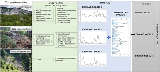
3. Monitoring Methods

The current monitoring network consists of the remote-sensing GNSS, in situ geotechnical sensors (wire extensometer, piezometers, and inclinometers), and a rain gauge (Figure 1 and Figure 3). Selecting the most suitable monitoring techniques has been challenging due to the extent of the study area, the site configuration, and the densely vegetated surface. We also had to consider the cost of monitoring techniques and multiple logistical constraints (no electricity, difficult access, limited signal service). Based on previous research and detailed field investigations, and taking into account all constraints, we selected the monitoring techniques that we considered most useful in our efforts to monitor the dynamics of the Urbas landslide.

3.1. Remote Sensing

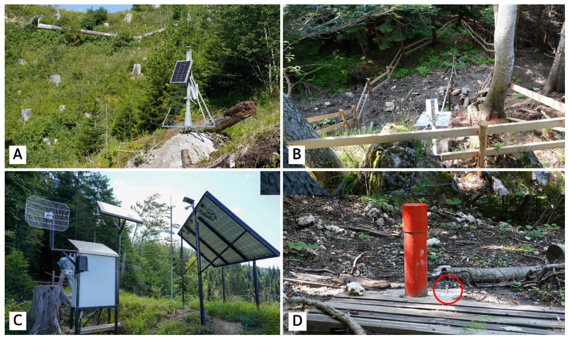
3.1.1. GNSS

Innovative, self-sufficient monitoring units equipped with low-cost dual-frequency GNSS antennae were permanently installed in four fixed locations across the landslide body to measure surface displacements (Figure 3A), and a local reference unit was installed outside of it [39,40]. The GNSS system has several advantages for deploying monitoring units in inaccessible locations and continuously monitoring with real-time data transfer. However, the deployment is limited to locations with open sky, which made the installation in the central, forested part of the landslide impossible. The position of monitoring points was calculated with a precision of 1 mm on the horizontal and 2 mm on the vertical axis by employing an open-source application and delivered daily through an FTP server in real time.

3.1.2. UAV Photogrammetry

UAV photogrammetry has become widely used for acquiring remote sensing data to monitor landslides. This approach provides high-resolution imagery from which dense point clouds, high-resolution digital elevation models, and orthophotos can be produced. In addition, UAV photogrammetry bridges the gap in scale, resolution, and viewing angle between terrestrial observation and satellite sensors [41,42]. Although UAV-photogrammetry-derived data cannot provide a highly accurate or real-time state of the instability, they can cover a wider landslide area rather than just specific observation points, thereby contributing to a considerably better understanding of the landslide kinematics. Recently, UAV photogrammetry has been successfully applied to landslide mapping and monitoring [21,43,44,45,46,47,48]. However, its applicability is limited to non-vegetated areas [49].

To evaluate surface changes in elevation and the volume of deposited dry gravel material in the non-vegetated upper part of the Urbas landslide (Figure 2A), three periodic measurements were performed using UAV photogrammetry. The upper part above the main scarp is characterized by a steep slope of carbonate rock, prone to rapid physical and chemical weathering due to lithological and structural conditions. This results in large amounts of accumulated dry gravel in the form of four alluvial fans that cover the area of the main scarp and below. This part is dominated by rockfalls, rockslides, and dry gravel runoff [21,31].

Acquisitions of UAV images of the monitoring site were conducted in September 2019, May 2020, and September 2020, and were limited only to the unvegetated area of the Urbas landslide (Figure 1). Surveys were conducted using a DJI Phantom 4 Pro equipped with a 20-megapixel camera. UAV point clouds were georeferenced using 10 ground control points (GCPs) deployed over accessible areas of the monitoring site. The exact position of the GCPs was measured using tachymetry, which provided an accuracy of 2 mm. An assessment of landslide surface changes in elevation and volume as a result of displaced material was estimated by direct comparison of two successive, co-registered digital elevation models (DEMs). To examine the elevation differences, elevations from the earlier-acquired DEM were subtracted cell by cell from the later one.

3.2. In Situ Geotechnical Monitoring

3.2.1. Wire Extensometer

Because remote sensing techniques could not be used in the central part of the landslide due to dense vegetation, a wire extensometer was installed on the right flank of the landslide to monitor the opening of the lateral scarp (Figure 1). The wire extensometer is a simple device that measures a change in distance between two points (Figure 3B). It was installed at a lateral scarp along the slope, i.e., in the expected direction of the landslide displacements, with one point fixed at a relatively stable point outside the landslide body. It should be noted that the measured changes represented relative surface displacement of the landslide main body. Data with an accuracy of 1 mm were transmitted hourly in real time via the base station and the FTP server.

3.2.2. Piezometers

For groundwater table monitoring, six piezometers were installed. Three were analysed, since they were located in close proximity to the cross section A-A’ (Figure 1;

Table 1. Basic data for piezometers.

Piezometer	Ground Surface Altitude (m a.s.l.)	Depth (m)	Depth of Screened Interval (m)
P1	1289.2	21.0	6.9–18.9
P2	1232.4	15.0	2.5–5.5
			6.0–12.0
P3	1218.8	30.0	6.7–15.7

). Piezometer P1 was located in the upper part of the landslide and was close to the surface boundary of dry gravel and clastic rocks. The groundwater table was observed 13 m below the surface and rose up to 11.5 m during high-water conditions. The contact between gravel and underlying low permeable clastic rocks was at a depth of 18 m. Piezometers P2 and P3 were in the main body of the landslide. The low groundwater table in these piezometers was at depths of 3 m and 3.5 m, respectively. Higher fluctuations of the groundwater table were observed, up to 2 m in piezometer P2 and up to 3 m in P3.

3.2.3. Inclinometers

The implementation of inclinometers is required for determining the depth of the sliding surface and to monitor the magnitude, rate, and direction of landslide displacement [9,50]. A total of six were installed at the Urbas landslide [31]. In this research, two inclinometers (I1 and I2) located in proximity to the A–A’ cross section (Figure 1) were analysed. The measurements were carried out using an RST MEMS digital inclinometer probe with a measurement interval of 0.5 m. The entire apparatus consisted of the probe, a heavy-duty control cable wound onto a slip-ring reel, and KLION software (SISGEO, Masate, Italy). PVC inclinometer casings have longitudinal grooves in two perpendicular directions (A and B) to ensure that the probe remains oriented in the desired direction, in this case, the expected movement direction of the Urbas landslide.

3.3. Geodetic Monitoring

To assess the reliability of the displacements obtained by remote sensing, it was important to compare them with known reference measurements [49]. To verify displacements obtained from the GNSS and to determine the absolute displacements of the landslide, classic tachymetric geodetic measurements using a theodolite were performed simultaneously with the acquisition of the inclinometer data (Figure 1). The high positional and height accuracy of the tachymetric geodetic measurements (±2 mm) allowed an accurate assessment of the displacements of object points installed at the boreholes (Figure 3). We observed measurements of the five object points installed along the A-A’ cross-section (Figure 1).

4. Results

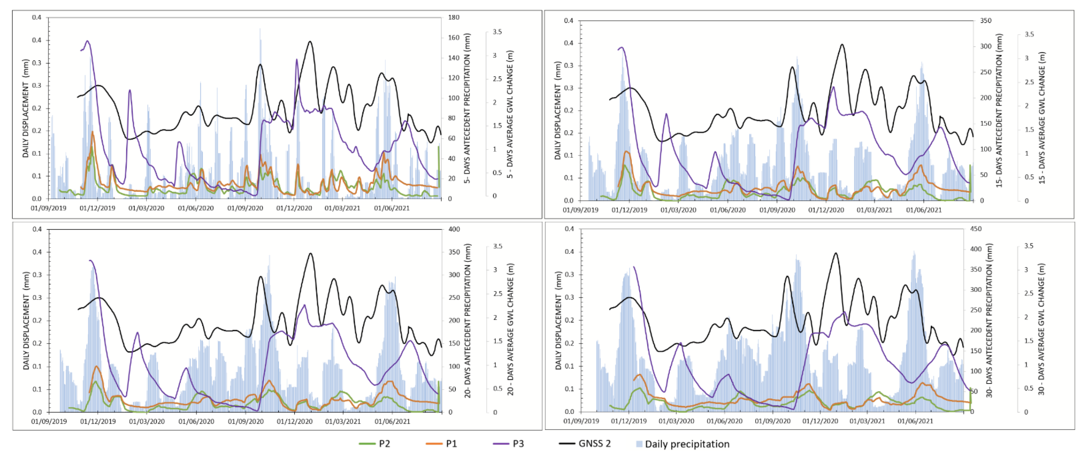
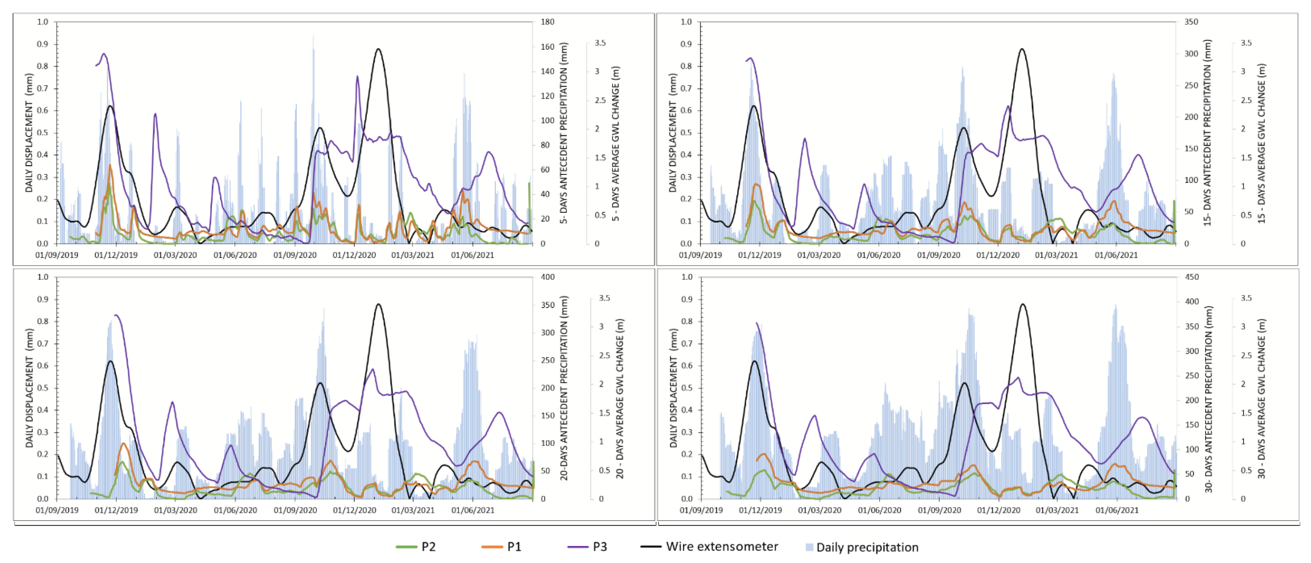
4.1. Surface Displacements

Continuous surface displacement monitoring obtained by GNSS was analysed for the 22-month period from October 2019 to the end of August 2021, while the wire extensometer monitoring data were obtained for a two-year period from September 2019 until the end of August 2021 (Figure 1, Figure 4 and Figure 5). The GNSS and wire extensometer surface displacement rates were further verified and compared with tachymetric measurements of the object points (Figure 4 and Figure 5). It should be noted that the object points were not installed at the exact positions of the GNSS and the wire extensometer (Figure 1), but in their vicinity.

The upper part of the Urbas landslide consists of a slope covered by a large amount of dry gravel material that is prone to causing slope instability such as rockslides and runoff (Figure 1, Figure 2 and Figure 5). The core logging of the three boreholes and periodic inclinometer measurements showed that the depth of the sliding surface was around 23 m [25,31] (Figure 5). In the upper part of the Urbas landslide, the results of three GNSS and three object points were analysed (Figure 4). From the cumulative displacement curves, a linear or steady displacement trend was observed. The cumulative displacements for the monitoring period of 22 months were measured to be 121 (GNSS1), 135 (GNSS2), and 117 mm (GNSS3). The maximum daily displacement rates of GNSS were 0.32 (GNSS1), 0.35 (GNSS2). and 0.27 mm/day (GNSS3), while the monthly displacement rates were 1.7–7.4 (GNSS1), 4.0–8.8 (GNSS2), and 3.4–7.0 mm/month (GNSS3). The comparison with periodic measurements of the object points G1, P1, and I1, which are about 25 to 35 m away from the GNSS, also showed a similar trend. The displacement rates of the object points for the upper part of the landslide confirmed the linear sliding trend (Figure 5).

A wire extensometer monitored surface displacements on the right flank of the landslide main body, which consists of tectonically deformed and completely weathered clastic rocks, mainly siltstone and claystone. The sliding-surface depth was between 10 and 15 m [25,31] (Figure 5). Compared to the upper part, the main body is densely covered with coniferous forest, which prevented the installation of GNSS units, as mentioned above. The wire extensometer obtained continuous surface displacement data but, unlike the GNSS, the measured displacement values were relative because the wire extensometer could not be fixed to a stable point (Figure 1 and Figure 4). In contrast to the GNSS results for the upper part, the wire extensometer displacement curve showed periodic increasing (“steep like”) phases of landslide behaviour; the term was borrowed from [51]. The cumulative displacement for the 2-year monitoring period was 161 mm. The measured maximum daily displacement rate was 0.9 mm/day, while the average displacement rate was 0.1 mm/day. Two distinct acceleration phases, followed by an increasing linear displacement trend, were identified from the wire extensometer displacement curve. The first phase was from late October to middle November 2019, while the second was observed from December to January 2021. Periodic measurements of the object points (P3 and I2) indicated a similar trend to the wire extensometer displacement curve, but with much higher displacement rates. Object point P3 was subjected to a surface displacement of 71.7 mm for about 5 months from April to September 2020 and 263.3 mm for the 9 months from September 2020 to June 2021. Object point I2 indicated the following monitoring period displacement rates: 64.5 mm from January to April 2020, 84.2 mm from April to September 2020, and 253.2 mm from September 2020 to June 2021. In contrast to the wire extensometer, both object points detected significant displacement especially during the winter, which were estimated at about 28 to 29 mm/month. The discrepancy between the results was probably related to the position of the sensors. The object points were located in the landslide main active body area, while the wire extensometer was located on the edge of the right flank (Figure 1). The distance between them is about 210 m. The second reason for the displacement rate discrepancy was that the wire extensometer measured relative displacements, while the object points gave absolute displacement values with high accuracy.

The toe of the Urbas landslide is considered to be the most active part. It consists of tectonically deformed and decomposed clastic rocks mixed with a large amount of carbonate talus material. In addition, the Bela stream causes erosion and contributes significantly to the mobilization of sliding material downstream [25,31]. Due to its gully-type morphology and difficult site accessibility, it was not possible to install geotechnical equipment (boreholes and wire extensometer) in situ. For this reason, only one GNSS (GNSS4) was used for landslide monitoring (Figure 1 and Figure 4). However, GNSS monitoring also confirmed strong landslide activity, as the toe experienced significantly larger displacement rates compared to the upper part and the main body. The cumulative displacement at the landslide toe was 739 mm for the 22-month monitoring period. The maximum daily displacement was 4.5 mm/day, while the average rate was 1.1 mm/day. The cumulative displacement curve obtained by GNSS and the wire extensometer showed a combination of steady-growth displacement trends and “steep like” phases. The first significant acceleration phase was detected from October to December 2019, while the second one was observed from late November 2020 to late February 2021.

The displacement curves for the landslide main body and toe suggest that steep-like phases may be related to external triggering factors such as precipitation and changes in groundwater tables. The correlation with surface displacements and hydrometeorological parameters is analysed further in Section 3.1.1 and Section 3.1.2

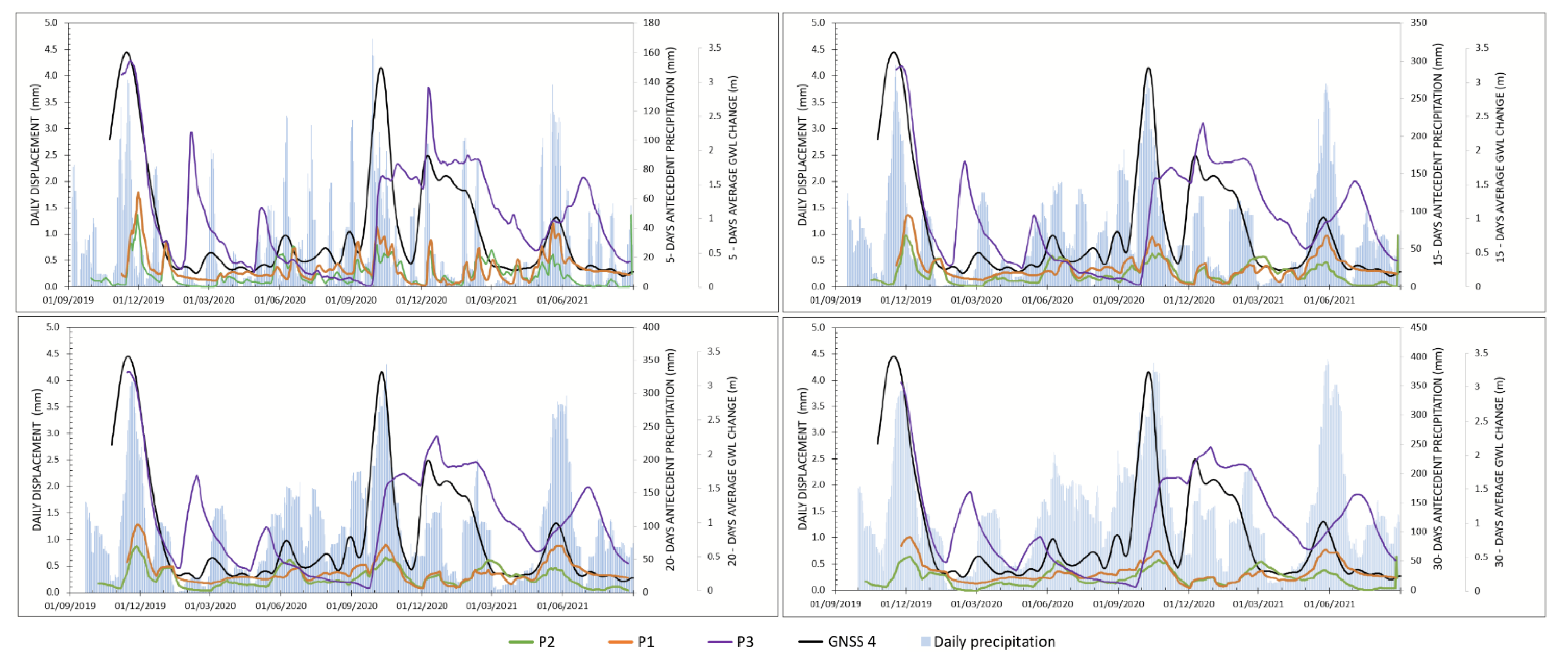
Interrelation of the Landslide Displacement Rate, Precipitation, and Groundwater Level Change

Landslide trigger mechanism detection and dynamics evaluation were performed by analysing the response relation among displacement, antecedent precipitation, and groundwater table change. Time-series graphs of continuous monitoring data were plotted and showed the rate of daily surface displacement; 5-, 15-, 20-, and 30-day antecedent precipitation; and 5-, 15-, 20-, and 30-day average changes in the groundwater table (Figure 5, Figure 6 and Figure 7). Based on the cumulative displacement curves (Figure 4), the time-series analysis of relationship level was distinguished separately for the landslide upper part (Figure 6), main body (Figure 7), and toe (Figure 8).

Daily precipitation was obtained by rain gauge at the landslide. During the period from September 2019 to the end of August 2021, the Urbas landslide experienced a combination of long rainy and dry periods. It should be noted that extreme rainfall events, normally characteristic for this part of Slovenia, were not recorded during this monitoring period and, therefore, their influence could not be detected. Following other studies [51,52,53] in which the dynamics of deep-seated landslides were assumed to be related to long-term antecedent precipitation rather than to short, intense precipitation, we decided to observe the correlation with the 5-, 15-, 20-, and 30-day antecedent precipitation.

Groundwater table monitoring data were obtained by three piezometers (Figure 1, Table 1) and were represented as a daily change calculated for 5-, 15-, 20-, and 30-day averages. The changes in the groundwater table of P1, P2, and P3 showed different groundwater dynamics, reflecting the complex hydrogeological conditions of the study area. Strong groundwater fluctuation was observed in piezometer P3 where the groundwater table oscillated up to 3 m, from a depth of 10 to 7 m. Groundwater fluctuations in piezometers P1 and P2 showed similar dynamics, strongly related to meteorological conditions. Groundwater table response to rain events is characterized by rapid rising and falling. The fluctuation amplitude was up to around 1.5 m.

Analysis of daily displacement rates measured at different parts of the Urbas landslide showed different patterns, confirming the assumption that the landslide is composite and prone to different dynamics. As expected, the highest displacement rates were recorded in the lower part of the landslide, where a maximum of 4.45 mm/day was observed (Figure 6). A similar pattern with lower displacement rates was observed at the landslide main body where the maximum displacement rate was 0.88 mm/day. The largest deviation in daily displacement detected by the extensometer and GNSS4 was observed from December 2020 to March 2021. During this period, the extensometer showed an average displacement acceleration of 0.03 mm/day, while GNSS4 indicated a more linear displacement. The discrepancy between the results is likely related to the effects of snow. During the same period, a high groundwater table of about 1 m was observed in piezometer P3, which could be related to snowmelt.

Lower displacement rates with smaller fluctuations were recorded at the upper part of the landslide, with a maximum daily displacement rate of 0.35 mm/day (Figure 6).

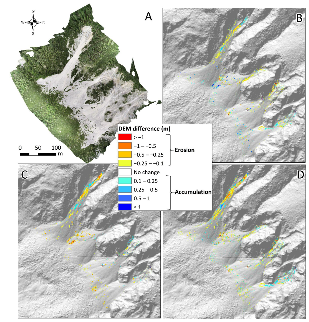
4.2. The Impact of Steep-Slope Erosion above the Main Scarp

To estimate the rate of erosion and accumulation of talus material above the Urbas landslide main scarp, three periodic measurements were performed using UAV photogrammetry. To examine elevation differences between two successive DEMs, elevations from the earlier-acquired DEM were subtracted from the later acquisition on a cell-by-cell basis with a cell resolution of 0.1 m. In the present study, one of the main disadvantages of UAV photogrammetry was the dense vegetation covering the upper part of the landslide because it hindered reliable photogrammetric processing and the derivation of surface models. Consequently, observations of elevation change were limited to the non-vegetated areas. Assessments of elevation and volume changes were calculated for 31,452 m², the analysed area (Figure 9).

For the first observation period (fall and winter), a comparison of September 2019 to May 2020 was made (Figure 9B,

Table 2. Calculated changes between subsequent DEMs.

	Area (m2)			Volume Change (m3)
DEM Diff.	Erosion	Accumulation	No Change	Erosion	Accumulation
10 Aug 2019–14 May 2020	1846	1350	28,256	881	806
14 May 2020–19 Aug 2020	1806	528	29,118	890	431
10 Aug 2019–19 Aug 2020	2838	1186	27,428	1230	695

). The comparison showed that the total area of erosion within the analysed area was 1846 m² (approximately 6%), while the total area of accumulation was 1350 m² (approximately 4% of the analysed area). No elevation changes were observed in the largest part of the analysed area (28,256 m²). The first observation period showed that erosion was predominant in the upper part, where the elevation decreased from 0.5 to 1 m. As expected, sediment accumulation was observed in the middle and lower parts. The volume of the eroded surface material amounted to 881 m³, and that of the accumulated material to 806 m³. No significant deficit was observed during this period.

In the following period (spring) between May 2020 and August 2020 (Figure 9C, Table 2), 1806 m² (about 6% of the analysed area) was affected by erosion, and the surface had subsided by 0.5 m on average. An insignificant part of the analysed area (about 2%) was characterized by accumulation, with an average increase of 0.25 and a maximum increase of 1 m. No elevation changes were observed within an area of 29,118 m² (92%). A volume loss of 890 m³ and an accumulation of 431 m³ were calculated.

The comparison between August 2019 and August 2020 showed significant changes in the northwestern part. An area of about 2800 m² (about 10%) was characterised by erosion, while only 4% (1190 m²) was dominated by the accumulation of material. No elevation changes were observed in the majority of the area (86%). The results indicated a predominance of erosion in the northwestern part of the studied area. Localised areas of significant elevation change could have been the result of rock falls. The total volume of eroded material was estimated at 1230 m³, while the volume of accumulated material over a 1-year period was estimated at 695 m³. The deficit was apparently transported downslope outside the area.

5. Discussion

As described in Section 3.1.1 and Section 3.1.2, the Urbas landslide exhibited different kinematic trends associated with different triggering mechanisms. To find out which external triggering factors were the most strongly related to surface displacement, the correlation between daily surface displacements and the hydrometeorological parameters of cumulative daily precipitation and average groundwater table was calculated (

Table 3. Pearson correlation coefficient (r) between daily surface displacements and hydrometeorological parameters.

Hydrometeorological Parameters		Correlation Coefficient (r)
		GNSS2	Wire Extensometer	GNSS4
5	-days antecedent precipitation	0.27	0.19	0.41
10		0.33	0.24	0.49
15		0.35	0.28	0.53
20		0.37	0.29	0.54
30		0.39	0.29	0.52
5	piezometer P1 -days average GWL change	0.32	0.21	0.55
10		0.34	0.22	0.58
15		0.35	0.22	0.59
20		0.34	0.21	0.57
30		0.29	0.15	0.47
5	piezometer P2 -days average GWL change	0.42	0.23	0.48
10		0.45	0.24	0.48
15		0.47	0.24	0.46
20		0.47	0.23	0.43
30		0.43	0.20	0.35
5	piezometer P3 -days average GWL change	0.40	0.54	0.65
10		0.41	0.56	0.63
15		0.41	0.56	0.60
20		0.41	0.56	0.55
30		0.41	0.51	0.44

). For correlation analysis, the Pearson coefficient was used, while its interpretation was based on [54].

The results (Section 3) revealed that the Urbas landslide dynamics varied along the landslide area, mainly depending on local geological and hydrogeological conditions. Consequently, certain parts of the landslide are at different evolutionary states and respond differently to the same external trigger factors.

GNSS surface displacements and in situ geotechnical investigations indicated that the upper part is a steady-type landslide, a term borrowed from [44]. Surface displacements increased monotonically with time, with average displacement rates of about 5.5 mm per month, whereas deep displacements (obtained from I1) were observed at a contact between dry gravel and decomposed clastic rocks at a depth of 23 mm, with a change rate of about 55 mm in 11 months. The linear displacement trend and correlation coefficients indicated that the landslide dynamics of the upper part are controlled by internal controlling factors such as the lithology, morphology, and gravity of the dry gravel material load (Figure 6, Table 1). Their dependence on external triggering factors such as precipitation and groundwater table change is insignificant. The impact assessment of erosion using UAV photogrammetry showed that there was no significant contribution of material from the slope above the main scarp during the period between August 2019 and May 2020.

In contrast to the landslide upper part, the cumulative displacement curves for the main body indicated that the dynamics were the result of a combination of slow-moving steady landslide and episodic steep-like displacements that corresponded to external triggering factors (Figure 4). An analysis of the relation among surface displacements, precipitation, and groundwater table changes showed that the highest correlation coefficient was found between surface displacements obtained by a wire extensometer and groundwater table change observed in the P3 piezometer (Figure 7, Table 3). The reason was that the groundwater table fluctuation in P3 reflected the hydrological conditions in the deeper part of the landslide (Table 1). This was consistent with the finding that main-body landslide dynamics is related to deep displacements observed at a depth of 10 m (obtained from the I2) at the contact between residual soil and decomposed clastic rock. A periodic trend of increased surface and deep displacement rates, as well as the correlation analysis, indicated that the dynamics in this part are related to the groundwater level fluctuation in piezometer P3 and consequently to the saturation of the residual soil (Figure 4 and Figure 7, Table 3). The correlation analysis also indicated that displacement could have delayed response to groundwater table change, possibly because the landslide is deep-seated and consists mainly of clastic rocks with low soil permeability. The change in the groundwater table and precipitation both showed seasonal patterns and had a complex relationship with surface displacement.

The toe was recognized as the most active part of the landslide. The sliding mass in this part consisted of decomposed and saturated clastic rocks mixed with a large amount of scree material and vegetation remains. The area is crossed by the Bela stream, which causes erosion and contributes significantly to the mobilization of the sliding material downstream [25,31]. The dynamics of the landslide toe are consequently related to precipitation and increased discharge from the Bela and its tributaries. This is also indicated by a correlation analysis showing that surface displacement could be correlated with precipitation, especially after 20 days of antecedent precipitation (Figure 8, Table 3). This suggests that long-term precipitation (20 days to 1 month) can increase the displacement rate. The correlation analysis also showed that groundwater table fluctuations also had an influence on the surface displacement of GNSS4 (Figure 8, Table 3). The reason was that piezometer P1 measured the groundwater table in an aquifer that recharges the Urbas spring. The Urbas spring feeds the Bela stream, which flows, uncontrolled, along the landslide and influences the shallow hydrogeological conditions that were observed in piezometer P2.

The surface displacement analysis and the correlation between the daily displacements and the external triggering factors indicated that there was weak correlation among surface displacements, cumulative daily precipitation, and average groundwater table during the 2-year monitoring period from September 2019 to September 2021. It should be taken into account that the period of continuous monitoring was relatively short and that there were none of the significant precipitation events typical for this area. A review of recent meteorological data showed that there was no precipitation event of the magnitude of the April 2017 event (approximately 200 mm/48 h) that could cause a debris flow in the immediate vicinity of the Urbas landslide [23,26]. This reinforces the need to continue the monitoring system to gain better insight into landslide dynamics and the influence of external factors. Further investigation should also consider the influence of snow, which was not addressed in this study due to lack of available snow-cover data such as depth and water equivalent.

6. Conclusions

From this study, six main outcomes were derived.

• Real-time surface displacements obtained from continuous monitoring using GNSS proved to be essential input data for landslide dynamics assessment and allowed us to obtain information on landslide kinematics.
• In situ electronic geotechnical devices (a wire extensometer in our case) show real time displacement trends comparable to those obtained by the GNSS method and could also serve as an internal control of the GNSS monitoring. The use of geotechnical devices on the site is less constrained by topography (open sky) and vegetation but shows a greater impact of external factors such as temperature variations, snow cover, and lightning strikes that need to be considered in data analysis.
• GNSS provided a cost-effective and easy-to-use method for monitoring landslide kinematics, but conventional in situ geotechnical and geodetic equipment and surveys are still essential for obtaining information about the depth of the sliding surface and groundwater dynamics.
• Additional remote sensors to allow continuous monitoring of surface displacements are required, especially on the main body of landslide. The monitoring network could be upgraded with additional in situ geotechnical equipment such as inclinometers because the current ones were destroyed due to landslide activity. Continuous measurement of the Bela stream flow would also add to the knowledge of the influence of surface water on landslide dynamics, especially in the area of the landslide toe, which is prone to debris flow.
• Before being implemented, new monitoring methods need to take into account constraints that could cause scattering for remote sensing: landslide orientation (northeast to southwest), area size, vegetation, lack of power supply and absence of infrastructure.
• Recent studies in Slovenia have shown that the frequency and intensity of precipitation events are expected to increase because of climate change [3], so the total and effective amount of rainfall, air temperature, evapotranspiration, and runoff from the Bela stream catchment are expected to increase [37].

References

- Haque, U.; Blum, P.; Da Silva, P.F.; Andersen, P.; Pilz, J.; Chalov, S.R.; Malet, J.-P.; Auflič, M.J.; Andres, N.; Poyiadji, E. Fatal landslides in Europe. Landslides 2016, 13, 1545–1554. [Google Scholar] [CrossRef]
- Herrera, G.; Mateos, R.M.; García-Davalillo, J.C.; Grandjean, G.; Poyiadji, E.; Maftei, R.; Filipciuc, T.-C.; Auflič, M.J.; Jež, J.; Podolszki, L. Landslide databases in the Geological Surveys of Europe. Landslides 2018, 15, 359–379. [Google Scholar] [CrossRef]
- Auflič, M.J.; Bokal, G.; Kumelj, Š.; Medved, A.; Dolinar, M.; Jež, J. Impact of climate change on landslides in Slovenia in the mid-21st century. Geologija 2021, 64, 159–171. [Google Scholar] [CrossRef]
- Jemec Auflič, M.; Jež, J.; Popit, T.; Košir, A.; Maček, M.; Logar, J.; Petkovšek, A.; Mikoš, M.; Calligaris, C.; Boccali, C. The variety of landslide forms in Slovenia and its immediate NW surroundings. Landslides 2017, 14, 1537–1546. [Google Scholar] [CrossRef]
- Froude, M.J.; Petley, D.N. Global fatal landslide occurrence from 2004 to 2016. Nat. Hazards Earth Syst. Sci. 2018, 18, 2161–2181. [Google Scholar] [CrossRef] [Green Version]
- Gariano, S.L.; Guzzetti, F. Landslides in a changing climate. Earth-Sci. Rev. 2016, 162, 227–252. [Google Scholar] [CrossRef] [Green Version]
- Lacroix, P.; Handwerger, A.L.; Bièvre, G. Life and death of slow-moving landslides. Nat. Rev. Earth Environ. 2020, 1, 404–419. [Google Scholar] [CrossRef]
- Li, H.; Xu, Q.; He, Y.; Deng, J. Prediction of landslide displacement with an ensemble-based extreme learning machine and copula models. Landslides 2018, 15, 2047–2059. [Google Scholar] [CrossRef]
- Chae, B.-G.; Park, H.-J.; Catani, F.; Simoni, A.; Berti, M. Landslide prediction, monitoring and early warning: A concise review of state-of-the-art. Geosci. J. 2017, 21, 1033–1070. [Google Scholar] [CrossRef]
- Huang, F.; Huang, J.; Jiang, S.; Zhou, C. Landslide displacement prediction based on multivariate chaotic model and extreme learning machine. Eng. Geol. 2017, 218, 173–186. [Google Scholar] [CrossRef]
- Gao, W.; Dai, S.; Chen, X. Landslide prediction based on a combination intelligent method using the GM and ENN: Two cases of landslides in the Three Gorges Reservoir, China. Landslides 2020, 17, 111–126. [Google Scholar] [CrossRef]
- Li, X.; Kong, J.; Wang, Z. Landslide displacement prediction based on combining method with optimal weight. Nat. Hazards 2012, 61, 635–646. [Google Scholar] [CrossRef]
- Arbanas, S.M.; Arbanas, Ž. Landslides: A guide to researching landslide phenomena and processes. In Transportation Systems and Engineering: Concepts, Methodologies, Tools, and Applications; IGI Global: Hershey, PA, USA, 2015; pp. 1393–1428. [Google Scholar]
- Uhlemann, S.; Smith, A.; Chambers, J.; Dixon, N.; Dijkstra, T.; Haslam, E.; Meldrum, P.; Merritt, A.; Gunn, D.; Mackay, J. Assessment of ground-based monitoring techniques applied to landslide investigations. Geomorphology 2016, 253, 438–451. [Google Scholar] [CrossRef] [Green Version]
- Pecoraro, G.; Calvello, M.; Piciullo, L. Monitoring strategies for local landslide early warning systems. Landslides 2019, 16, 213–231. [Google Scholar] [CrossRef]
- Mikoš, M. After 2000 Stože Landslide: Part I–Development in landslide research in Slovenia. Acta Hydrotech. 2020, 33, 129–153. [Google Scholar] [CrossRef]
- Mikoš, M. After 2000 Stože Landslide: Part II-Development of landslide disaster risk reduction policy in Slovenia. Acta Hydrotech. 2021, 34, 39–59. [Google Scholar] [CrossRef]
- Krkač, M.; Špoljarić, D.; Bernat, S.; Arbanas, S.M. Method for prediction of landslide movements based on random forests. Landslides 2017, 14, 947–960. [Google Scholar] [CrossRef]
- Krkač, M.; Bernat Gazibara, S.; Arbanas, Ž.; Sečanj, M.; Mihalić Arbanas, S. A comparative study of random forests and multiple linear regression in the prediction of landslide velocity. Landslides 2020, 17, 2515–2531. [Google Scholar] [CrossRef]
- Zhao, C.; Lu, Z. Remote sensing of landslides—A review. Remote Sens. 2018, 10, 279. [Google Scholar] [CrossRef] [Green Version]
- Peternel, T.; Kumelj, Š.; Oštir, K.; Komac, M. Monitoring the Potoška planina landslide (NW Slovenia) using UAV photogrammetry and tachymetric measurements. Landslides 2017, 14, 395–406. [Google Scholar] [CrossRef]
- Cruden, D.M.; Varnes, D.J. Landslides: Investigation and Mitigation. Chapter 3—Landslide Types and Processes; 030906208X; National Research Council: Washington, DC, USA, 1996; pp. 36–75. [Google Scholar]
- Jež, J.; Mikoš, M.; Trajanova, M.; Kumelj, Š.; Budkovič, T.; Bavec, M. Vršaj Koroška Bela-Rezultat katastrofičnih pobočnih dogodkov (Koroška Bela alluvial fan-The result of the catastrophic slope events; Kaeavanke Mountains, NW Slovenia). Geologija 2008, 51, 8. [Google Scholar] [CrossRef]
- Jemec Auflič, M.; Kumelj, Š.; Peternel, T.; Jež, J. Understanding of landslide risk through learning by doing: Case study of Koroška Bela community, Slovenia. Landslides 2019, 16, 1681–1690. [Google Scholar] [CrossRef] [Green Version]
- Peternel, T.; Jež, J.; Milanič, B.; Markelj, A.; Jemec Auflič, M. Engineering-geological conditions of landslides above the settlement of Koroška Bela (NW Slovenia). Geologija 2018, 61, 177–189. [Google Scholar] [CrossRef]
- Janža, M.; Serianz, L.; Šram, D.; Klasinc, M. Hydrogeological investigation of landslides Urbas and Čikla above the settlement of Koroška Bela (NW Slovenia). Geologija 2018, 61, 191–203. [Google Scholar] [CrossRef]
- Bezak, N.; Sodnik, J.; Maček, M.; Jurček, T.; Jež, J.; Peternel, T.; Mikoš, M. Investigation of potential debris flows above the Koroška Bela settlement, NW Slovenia, from hydro-technical and conceptual design perspectives. Landslides 2021, 18, 3891–3906. [Google Scholar] [CrossRef]
- Jež, J.; Peternel, T.; Milanič, B.; Markelj, A.; Novak, M.; Celarc, B.; Janža, M.; Jemec Auflič, M. Čikla landslide in Karavanke Mts. (NW Slovenia). In Proceedings of the 4th Regional Symposium on Landslides in the Adriatic—Balkan Region, Sarajevo, Bosnia and Herzegovina, 23–25 October 2019; pp. 239–242. [Google Scholar]
- Lavtižar, J. Zgodovina Župnij in Zvonovi v Dekaniji Radolica; (in Slovenian). Self-published by Lavtižar, J.: Ljubljana, Slovenia, 1897; p. 148. [Google Scholar]
- Zupan, G. Krajevni Leksikon Dravske Banovine; Uprava Krajevnega leksikona dravske banovine Ljubljana: Ljubljana, Slovenia, 1937; p. 540. [Google Scholar]
- Peternel, T.; Jež, J.; Janža, M.; Šegina, E.; Zupan, M.; Markelj, A.; Novak, A.; Jemec Auflič, M.; Logar, J.; Maček, M.; et al. Mountain slopes above Koroška Bela (NW Slovenia)—A landslide prone area. In Proceedings of the 5th Regional Symposium on Landslides in the Adriatic-Balkan Region, Rijeka, Croatia, 23–26 March 2022; pp. 13–18. [Google Scholar]
- Koren, K.; Serianz, L.; Janža, M. Characterizing the Groundwater Flow Regime in a Landslide Recharge Area Using Stable Isotopes: A Case Study of the Urbas Landslide Area in NW Slovenia. Water 2022, 14, 912. [Google Scholar] [CrossRef]
- Peternel, T.; Šegina, E.; Zupan, M.; Auflič, M.J.; Jež, J. Preliminary Result of Real-Time Landslide Monitoring in the Case of the Hinterland of Koroška Bela, NW Slovenia. In Proceedings of the Workshop on World Landslide Forum, Kyoto, Japan, 3 November 2020; pp. 459–464. [Google Scholar]
- Komac, M.; Holley, R.; Mahapatra, P.; van der Marel, H.; Bavec, M. Coupling of GPS/GNSS and radar interferometric data for a 3D surface displacement monitoring of landslides. Landslides 2015, 12, 241–257. [Google Scholar] [CrossRef]
- Komac, M.; Peternel, T.; Auflič, M.J. TXT-tool 2.386-2.1: SAR Interferometry as a Tool for Detection of Landslides in Early Phases. In Landslide Dynamics: ISDR-ICL Landslide Interactive Teaching Tools; Sassa, K., Guzzetti, F., Yamagishi, H., Arbanas, Ž., Casagli, N., McSaveney, M., Dang, K., Eds.; Springer: Berlin/Heidelberg, Germany, 2018; pp. 275–285. [Google Scholar]
- Peternel, T. Dinamika Pobočnih Masnih Premikov na Območju Potoške Planine z Uporabo Rezultatov Daljinskih in Terestričnih Geodetskih Opazovanj ter In-Situ Meritev: Doktorska Disertacija. Ph.D. Thesis, Univerza v Ljubljani, Naravoslovnotehniška fakulteta, Ljubljana, Slovenia, 2017. [Google Scholar]
- Bezak, N.; Peternel, T.; Medved, A.; Mikoš, M. Climate Change Impact Evaluation on the Water Balance of the Koroška Bela Area, NW Slovenia. In Proceedings of the Workshop on World Landslide Forum, Kyoto, Japan, 3 November 2020; pp. 221–228. [Google Scholar]
- Peternel, T.; Jež, J.; Milanič, B.; Markelj, A.; Sodnik, J.; Maček, M.; Jemec Auflič, M. Implementation of multidisciplinary approach for determination of landslide hazard. In Proceedings of the World Construction Forum 2019, Ljubljana, Slovenia, 8–11 April 2019; p. 124. [Google Scholar]
- Šegina, E.; Peternel, T.; Urbančič, T.; Realini, E.; Zupan, M.; Jež, J.; Caldera, S.; Gatti, A.; Tagliaferro, G.; Consoli, A. Monitoring Surface Displacement of a Deep-Seated Landslide by a Low-Cost and near Real-Time GNSS System. Remote Sens. 2020, 12, 3375. [Google Scholar] [CrossRef]
- Šegina, E.; Jemec Auflič, M.; Peternel, T.; Zupan, M.; Jež, J.; Realini, E.; Colomina, I.; Crosetto, M.; Consoli, A.; Luca, S. Validation and interpretation of data obtained by the newly developed low-cost Geodetic Integrated Monitoring System (GIMS). In Proceedings of the EGU General Assembly Conference Abstracts, Vienna, Austria, 3–8 May 2020; p. 5170. [Google Scholar]
- Lucieer, A.; Jong, S.M.d.; Turner, D. Mapping landslide displacements using Structure from Motion (SfM) and image correlation of multi-temporal UAV photography. Prog. Phys. Geogr. 2014, 38, 97–116. [Google Scholar] [CrossRef]
- d’Oleire-Oltmanns, S.; Marzolff, I.; Peter, K.D.; Ries, J.B. Unmanned aerial vehicle (UAV) for monitoring soil erosion in Morocco. Remote Sens. 2012, 4, 3390–3416. [Google Scholar] [CrossRef] [Green Version]
- Turner, D.; Lucieer, A.; De Jong, S.M. Time series analysis of landslide dynamics using an unmanned aerial vehicle (UAV). Remote Sens. 2015, 7, 1736–1757. [Google Scholar] [CrossRef] [Green Version]
- Fernández, T.; Pérez, J.L.; Cardenal, J.; Gómez, J.M.; Colomo, C.; Delgado, J. Analysis of landslide evolution affecting olive groves using UAV and photogrammetric techniques. Remote Sens. 2016, 8, 837. [Google Scholar] [CrossRef] [Green Version]
- Godone, D.; Allasia, P.; Borrelli, L.; Gullà, G. UAV and structure from motion approach to monitor the maierato landslide evolution. Remote Sens. 2020, 12, 1039. [Google Scholar] [CrossRef] [Green Version]
- Devoto, S.; Macovaz, V.; Mantovani, M.; Soldati, M.; Furlani, S. Advantages of using UAV digital photogrammetry in the study of slow-moving coastal landslides. Remote Sens. 2020, 12, 3566. [Google Scholar] [CrossRef]
- Liu, B.; He, K.; Han, M.; Hu, X.; Ma, G.; Wu, M. Application of uav and gb-sar in mechanism research and monitoring of zhonghaicun landslide in southwest China. Remote Sens. 2021, 13, 1653. [Google Scholar] [CrossRef]
- Gaidi, S.; Galve, J.P.; Melki, F.; Ruano, P.; Reyes-Carmona, C.; Marzougui, W.; Devoto, S.; Pérez-Peña, J.V.; Azañón, J.M.; Chouaieb, H. Analysis of the geological controls and kinematics of the chgega landslide (Mateur, Tunisia) exploiting photogrammetry and InSAR technologies. Remote Sens. 2021, 13, 4048. [Google Scholar] [CrossRef]
- Stumpf, A.; Malet, J.-P.; Allemand, P.; Pierrot-Deseilligny, M.; Skupinski, G. Ground-based multi-view photogrammetry for the monitoring of landslide deformation and erosion. Geomorphology 2015, 231, 130–145. [Google Scholar] [CrossRef]
- Stark, T.D.; Choi, H. Slope inclinometers for landslides. Landslides 2008, 5, 339–350. [Google Scholar] [CrossRef]
- Miao, F.; Wu, Y.; Xie, Y.; Li, Y. Prediction of landslide displacement with step-like behavior based on multialgorithm optimization and a support vector regression model. Landslides 2018, 15, 475–488. [Google Scholar] [CrossRef]
- Bogaard, T.; Greco, R. Invited perspectives: Hydrological perspectives on precipitation intensity-duration thresholds for landslide initiation: Proposing hydro-meteorological thresholds. Nat. Hazards Earth Syst. Sci. 2018, 18, 31–39. [Google Scholar] [CrossRef] [Green Version]
- Yang, B.; Yin, K.; Lacasse, S.; Liu, Z. Time series analysis and long short-term memory neural network to predict landslide displacement. Landslides 2019, 16, 677–694. [Google Scholar] [CrossRef]
- Schober, P.; Boer, C.; Schwarte, L.A. Correlation coefficients: Appropriate use and interpretation. Anesth. Analg. 2018, 126, 1763–1768. [Google Scholar] [CrossRef] [PubMed]