Different Responses of Solar-Induced Chlorophyll Fluorescence at the Red and Far-Red Bands and Gross Primary Productivity to Air Temperature for Winter Wheat

Abstract

Solar-induced chlorophyll fluorescence (SIF) is closely related to the light-reaction process and has been recognized as a good indicator for tracking gross primary productivity (GPP). Nevertheless, it has not been widely examined how SIF and GPP respond to temperature. Here, we explored the linkage mechanisms between SIF and GPP in winter wheat based on continuous measurements of canopy SIF ($cSIF$), GPP, and meteorological data. To separately explore the structural and physiological mechanisms underlying the SIF–GPP relationship, we studied the temperature responses of the estimated light use efficiency ($LU{E}_p$), canopy-level chlorophyll fluorescence yield ($cSI{F}_{yield}$) and photosystem-level chlorophyll fluorescence yield (${\mathsf{\Phi }}_F$) estimated using canopy-scale remote sensing measurements. We found that GPP, red canopy SIF ($cSI{F}_{688}$) and far-red canopy SIF ($cSI{F}_{760}$) all exhibited a decreasing trend during overwintering periods. However, GPP and $cSI{F}_{688}$ showed relatively more obvious changes in response to air temperature ($T_a$) than $cSI{F}_{760}$ did. In addition, the $LU{E}_p$ responded sensitively to $T_a$ (the correlation coefficient, r = 0.83, p-value < 0.01). The $cSI{F}_{yield\_688}$ and ${\mathsf{\Phi }}_{F\_688}$ (${\mathsf{\Phi }}_F$ at 688 nm) also exhibited significantly positive correlations with $T_a$ (r > 0.7, p-value < 0.05), while $cSI{F}_{yield\_760}$ and ${\mathsf{\Phi }}_{F\_760}$ (${\mathsf{\Phi }}_F$ at 760 nm) were weakly correlated with $T_a$ (r < 0.3, p-value > 0.05) during overwintering periods. The results also show that $LU{E}_p$ was more sensitive to $T_a$ than ${\mathsf{\Phi }}_F$, which caused changes in the $LU{E}_p/{\mathsf{\Phi }}_F$ ratio in response to $T_a$. By considering the influence of $T_a$, the GPP estimation based on the total SIF emitted at the photosystem level ($tSIF$) was improved (with R² increased by more than 0.12 for $tSI{F}_{760}$ and more than 0.05 for $tSI{F}_{688}$). Therefore, our results indicate that the $LU{E}_p/{\mathsf{\Phi }}_F$ ratio is affected by temperature conditions and highlights that the SIF–GPP model should consider the influence of temperature.

1. Introduction

The photosynthetic fixed carbon process is a crucial biochemical activity that significantly affects the global carbon cycle [1,2]. However, gross primary productivity (GPP) sensitively responds to climate changes, such as a reduction in water availability and a general increase in air temperature. The accurate evaluation of GPP is still constrained by complex environmental conditions. Many studies have recently reported that solar-induced chlorophyll fluorescence (SIF) can track photosynthesis better than vegetation indices [3,4], providing us with a potential method to track GPP in complex environmental conditions.

The energy absorbed by plant chloroplasts is dissipated in three ways: photochemical quenching (abbreviated as PQ), nonphotochemical quenching (abbreviated as NPQ), and emitted SIF [5]. The energy distribution and transfer of the absorbed energy are crucial for linking SIF to GPP, whereas the energy distribution among PQ, SIF, and NPQ is largely influenced by environmental conditions. Temperature affects the photosynthetic capacity of plants through several complex biochemical processes [6]. Many overwintering species at higher latitudes experience a decline in photosynthetic rate due to chilling, especially for evergreen needle forests (ENF; [7,8]). The winter cold imposes thermodynamic constraints, slowing the enzymes related to the activities of PQ and the Calvin cycle; therefore, light-harvesting complexes (LHCs) cannot completely utilize the absorbed light for CO₂ fixation. Because photoinhibition susceptibility is stronger at low temperatures, a more severe decline in photosynthetic activity occurs when chilling is produced under high light [9,10]. NPQ is an important photoprotective mechanism that plays a role in protecting the photosystem II (PSII) from damage from cold temperatures [8,11]. The quantity of PsbS protein and carotenoids (particularly xanthophyll pigment and corresponding xanthophyll lutein cycle pigment) determines NPQ capacity [12,13,14]. At the leaf scale, Porcar-Castell et al. [6] reported that seasonal variation in fluorescence quantum yield was in agreement with the changes in the quantum yield of photochemistry (${\mathsf{\Phi }}_{PSII}$) for ENF throughout winter. At the canopy scale, Magney et al. [8] and Kim et al. [15] explored the temperature response of SIF and GPP in ENF. They found that SIF and GPP exhibited a decreasing trend during overwintering periods and demonstrated that NPQ played a key role in protecting plants from damage in winter. Overall, low temperatures affect the energy distribution, which further impacts the changes in SIF and GPP.

It is worth emphasizing that the GPP estimation based on canopy SIF is challenged by the mixed effects of structure and physiology. Due to scattering and reabsorption within leaves and canopies, the observed canopy SIF is not the true SIF emitted at the photosystem level (Figure 1). Therefore, the apparent fluorescence yield at the canopy level $(cSI{F}_{yield}$) may not be the real yield (the total fluorescence yield at the photosystem level, ${\mathsf{\Phi }}_F$). If the reabsorption process and scattering process are not appropriately addressed, erroneous physiological estimates may be deduced. Previous studies have suggested that SIF in the far-red band primarily responds to changes in canopy structure changes represented by the product of the photosynthetic active radiation (PAR) and the near-infrared reflectance ($NI{R}_{v}P$) rather than actual physiological changes in the fluorescence quantum yield for crop species [16]. In addition, some studies explored the dynamic changes between SIF and GPP in evergreen forests and found that SIF responded sensitively to PQ and NPQ [15,17]. It should be emphasized that the important abilities of SIF to track GPP are attributed to the potential physiological link between $LU{E}_p$ and ${\mathsf{\Phi }}_F$, which remains unclear, especially under environmental stresses [18]. To better underly the GPP–SIF relationship, it is necessary to investigate $LU{E}_p$, ${\mathsf{\Phi }}_F$ and the canopy escape probability of SIF ($f_{esc}$) separately [19]. GPP is generally calculated as the light use efficiency ($LU{E}_p$) multiplied by the absorbed photosynthetic active radiation (APAR) using a semiempirical LUE framework [20]:

$$GPP=APAR\times LU{E}_p$$

(1)

Similarly, canopy directional SIF ($cSIF$) can be expressed as the product of $cSI{F}_{yield}$ and APAR, which contains information on canopy escape efficiency ($f_{esc}$) and the photosystem fluorescence yield (${\mathsf{\Phi }}_F$):

$$cSIF=APAR\times cSI{F}_{yield}$$

(2)

$$cSI{F}_{yield}={\mathsf{\Phi }}_F\times f_{esc}$$

(3)

In addition, photosynthesis has two photosystems, named PSI and PSII. Both PSI and PSII are engaged in the emission spectrum for fluorescence in chloroplasts, which covers a wavelength range of 640–850 nm (Figure 1). However, the spectral characteristics between SIF emitted from PSI and PSII differ at the photosystem level and canopy level [4]. The fluorescence spectrum shape emitted from PSII has two peaks, with the magnitude of the left peak at 685 nm (red band) being substantially larger than the right peak at 740 nm (far-red band), but the fluorescence spectrum released from PSI only has one peak at 740 nm [21,22]. Due to the fact that the relative contribution of PSI fluorescence is generally modest and constant under changeable illumination, the fluorescence from PSI is frequently assumed to be stable, which is also the assumption of the SCOPE model (Soil Canopy Observation, Photochemistry and Energy fluxes) [23]. It should be noted that SCOPE is a 1D model and cannot accurately account for horizontal heterogeneity in the canopy. In addition, some studies have reported that the PSI activity is enhanced in overwintering plants [24]. Therefore, it is important to separate the portion of PSII and PSI in far-red SIF and red SIF to better understand the link mechanism between SIF and GPP under environmental stress conditions [25]. SIF emitted from PSII is susceptible to the PSII photochemistry, which is closely connected to carbon reactions [26].

Nevertheless, many studies only explored the physiological link between far-red SIF and GPP [27,28,29,30]. Kimm et al. [27] explored the physiological mechanism of far-red SIF and its unique potential for physiological stress detection based on a high-temperature experiment in a soybean field. They found that far-red SIF yield at the photosystem level (${\mathsf{\Phi }}_{F\_760}$) outperformed far-red SIF yield at the leaf level ($cSI{F}_{yield\_760}$) and ${\mathsf{\Phi }}_{F\_760}$ sensitively responded to the physiological downregulation of soybean gross primary productivity under high temperatures. Song et al. [28] evaluated the performance of the satellite SIF for winter wheat in response to heat stress and found that the $cSI{F}_{yield\_760}$ could provide a larger physiology-related stress response than $APAR$ and vegetation indices. Wang et al. [29] also reported that $cSI{F}_{yield\_760}$ can reasonably capture the spatial and temporal dynamics of drought and heatwave development and showed an earlier response than traditional vegetation indices (such as the enhanced vegetation index, EVI) during the early stages of drought and heatwave events. Recent studies have begun to explore the relationship between red SIF and GPP. For example, Goulas et al. [30] explored the apparent spectral fluorescence yields ($ASI{F}_{yield\_687}$ and $ASI{F}_{yield\_760}$, which were measured by SIF normalized with PAR) for wheat in correlation with GPP and found that far-red canopy SIF ($cSI{F}_{760}$) related more strongly to GPP than red canopy SIF ($cSI{F}_{688}$). It should be noted that $cSI{F}_{760}$ carries much information relating to the canopy structure, and Dechant et al. [16] reported that $NIRvP$ was a robust structural proxy for $cSI{F}_{760}$ and GPP across scales. At present, there are few studies on the relationship between red SIF and GPP under stress conditions. Therefore, in order to explore the physiological link between SIF and GPP under stress conditions, changes in both red and far-red SIF in response to environmental conditions should be explored.

Until now, except for ENF, the effects of temperature on the SIF–GPP relationship in most plants have not been well-explored [31]. Furthermore, some studies have found that plant function types influenced SIF–GPP relationships and that the impacts of low temperatures on photosynthetic apparatuses of woody plants (for example, ENF) and herbaceous species (for example, winter wheat) may follow a different pattern during the winter [32]. Therefore, observations on winter wheat would represent an important contribution to our knowledge of the impact of the differences between SIF and GPP in response to temperature.

Here, we studied the responses of red band and far-red band SIF as well as photosynthesis to low air temperature based on continuous measurements of winter wheat during the overwintering period. Furthermore, to disentangle the structural and physiological factors, we investigated the mechanisms linking GPP to SIF by disentangling the impacts of APAR, ${\mathsf{\Phi }}_F$ and $f_{esc}$, separately. Finally, we assessed the impacts of temperature on GPP estimation models based on SIF.

2. Materials and Methods

2.1. Experiment Site

Spectral and flux measurements were carried out at the Xiao Tangshan site in northern Beijing, China (XTS, 40°11′N, 116°27′E; Figure 2). At the XTS site, a tower-based platform was constructed in the crop field, which is planted with corn (Zea mays L.) in summer and winter wheat in autumn (Triticum aestivum L.). The XTS site is equipped with a comprehensive observation system, including flux, meteorological, hydrological, and spectral instruments [33].

The XTS site has a warm temperate continental semi-humid and semi-arid monsoon climate. The annual maximum temperature is above 25 °C, and the annual minimum temperature is below −10 °C. The average annual precipitation is about 600 mm. The soil type is loamy sandy according to the HWSD map and using the FAO 90 classification system [34]. In terms of the soil particle composition, in the surface (0–30 cm) soil layer, the clay content is 11%, the sand content is 83%, and the silt fraction is 6%. Fertilizer and irrigation were applied regularly. In this study, we used continuous measurements in winter wheat. The winter wheat generally grown in the north–south direction with a plant row spacing of about 12 cm.

2.2. Spectral Measurements

An auto-observation spectra system was installed on the 5 m tower-based platform (Bergsun Inc., Beijing, China). Over the course of the growing period of winter wheat, canopy spectra were continuously monitored by an Ocean Optics QE65pro spectrometer (QE65pro; Ocean Optics, Dunedin, FL, USA). The observation system covers a spectral range of 645–805 nm at a resolution of ~0.34 nm. The Ocean Optics QE65pro spectrometer samples at an interval of about 0.17 nm and has a high signal-to-noise ratio (SNR) greater than 1000 [35], which allows for better extraction of the fluorescence information. A cosine corrector (CC3-3-UV-S; Ocean Optics, Inc., Dunedin, FL, USA) and a conical fore-optic (bare fiber) were used to capture the downwelling incident radiance ($E\left(\lambda \right)$) and upwelling radiance ($L\left(\lambda \right)$), respectively. The former has a large field of view (FOV) of 180°, and the latter can make measurements within a small FOV of about 25°. In order to avoid the influence of the tower, the upwelling radiance was measured off-nadir with a view zenith angle of 25°. The ground instantaneous field of view (GIFOV) was close to 2.2 m. The GIFOV was used to describe the ground size observed by sensors ($GIFOV=2\ast \tan \left(FOV/2\right)\ast H$). In addition, the spectrometer uses a ‘sandwich’ type (the downwelling solar irradiance was first collected, the upwelling irradiance was then measured, and the downwelling solar irradiance was finally collected again by alternately opening the up and down channels) to reduce the influence of rapidly changing light conditions [36]. Moreover, the integration time can automatically be optimized depending on the light conditions. More details about the spectra observation system can be found in Du et al. [35]. The sowing date was 25 September 2020, and the harvest date was 5 June 2021. Finally, we gathered spectral data for the entire winter wheat growth cycle, from DOY 272 in 2020 to DOY 157 in 2021, for a total of 272 days.

2.3. Flux Measurements

The fluxes between plants and atmospheres were monitored by an eddy-covariance (EC) system, which was placed 5 m above the ground near the auto SIF observed system. The EC data were recorded at 10 HZ [37]. After detailed processing, the daytime partitioning algorithm was used to measure GPP using an online calculation tool (https://www.bgc-jena.mpg.debgiindex.php/Services/REddyProcWeb assessed on 1 June 2021) provided by the Max Planck Institute for Biogeochemistry, Germany (MPI-BGC) [38]. Therefore, we could further obtain the light use efficiency ($LU{E}_p$) based on Equation (1). In addition, an automatic weather station near the EC system was used to continuously measure PAR, air temperature ($T_a$), humidity (RH), air pressure, and other meteorological variables.

2.4. Data Processing

2.4.1. Estimation of $fPAR$

The $fPAR$ is the fraction of the incident photosynthetically active radiation (PAR) absorbed by vegetation, which was estimated using vegetation indices. Because the normalized difference vegetation index (NDVI) is susceptible to canopy structure and chloroplast absorption, it has been suggested to be proportional to $fPAR$ for a fixed view angle [39]. Generally, a large number of studies have used a simple linear model to estimate $fPAR$ by NDVI, whereas NDVI generally exhibited a saturation effect at a high LAI value. In order to eliminate the saturation effect of the NDVI, some studies have explored the performance of other vegetation indices as a proxy of $fPAR$, such as the wide-dynamic-range vegetation index (WDRVI) [40], which can be expressed as [41,42,43]:

$$WDRVI=\frac{\alpha \times Re{f}_{800}-Re{f}_{680}}{\alpha \times Re{f}_{800}+Re{f}_{680}}$$

(4)

where $Ref$ is the reflectance which was measured by the upwelling radiance divided by the downwelling radiance, and the subscript indicates the corresponding wavelength; $\alpha$ represents a weighting coefficient, which can be set to either 0.1 or 0.2 [42,44]. In this study, we used the value of 0.1 to represent $\alpha$ and calculated $WDRVI$ [44]. By using the value of 0.1 to represent $\alpha$, the WDRVI has been found to be closely related to $fPAR$ based on SCOPE simulation results (Figures S3 and S4) [41], thus we also used the existing linear model to estimate $fPAR$ using the WDRVI, which can be expressed as:

$$fPAR=0.516\times WDRVI+0.726$$

(5)

where the coefficients of 0.516 and 0.726 were taken from the literature by Liu et al. [41]. The absorbed photosynthetically active radiation (APAR) can be calculated as:

$$APAR=PAR\times fPAR$$

(6)

2.4.2. SIF Retrieval

Gases in the terrestrial or solar atmosphere result in strong absorption in spectral regions [45]. The relative contributions between reflected radiance and SIF provide us with an approach to retrieving SIF based on the spectrum (FLD), especially in the O₂ absorption bands [46]. Although the retrieved SIF based on the three-band (3FLD) algorithm is robust [47], it assumes that the reflectance in telluric O₂ absorption lines changes linearly and only uses limited bands. However, the spectral fitting method (SFM) takes advantage of the full features of wide-fitting windows [48]. Therefore, we used SFM to retrieve SIF from the vegetation radiation measurements. Here, we used a quadratic polynomial to parameterize SFM (Equation (7)), with an initial fitting window of 684.0–691.5 nm for the O₂B band and 757.0–772.5 for the O₂A band [49]. The quadratic formula is as follows [49,50]:

$$L\left(\lambda \right)=\left(b_5\Delta {\lambda }^2+b_4\mathsf{\Delta }\lambda +b_3\right)\frac{E\left(\lambda \right)}{\pi }+b_2\Delta {\lambda }^2+b_1\mathsf{\Delta }\lambda +b_0$$

(7)

where $b_{0-2}$ represents the fitted coefficients that can be used to model the fluorescence shape; $b_{3-5}$ represents the fitted coefficients that can be used to model the reflectance shape; $\lambda$ is the wavelengths in the fitting window, $\mathsf{\Delta }\lambda$ is the width of the fitting window; $L\left(\lambda \right)$ is the radiance reflected from the canopy; and $E\left(\lambda \right)$ is the irradiance downwelling from sky.

2.4.3. Estimation of $f_{esc}$ and ${\mathsf{\Phi }}_F$

We further obtained the canopy fluorescence quantum yield at the $\lambda$ band ($cSI{F}_{yield\_\lambda }$), which was equal to the canopy SIF at the $\lambda$ band ($cSI{F}_{\lambda }$) divided by APAR:

$$cSI{F}_{yield\_\lambda }=\frac{cSI{F}_{\lambda }}{APAR}$$

(8)

In addition, to study the physiology of fluorescence in relation to photosynthesis, we reduced the effects of the $f_{esc}$. The $f_{esc}$ at 760 nm ($f_{esc\_760}$) has been extensively studied [41,51,52,53]. Zeng et al. [54] proposed a simple formula that performs well at estimating of far-red $f_{esc}$ with extensive radiative transfer simulations, which can be expressed as:

$$NI{R}_v=Re{f}_{NIR}\times NDVI$$

(9)

$$f_{esc\_760}\approx \frac{NI{R}_v}{fPAR}$$

(10)

where $NI{R}_v$ is expressed as NIR reflectance multiplied by NDVI to represent the vegetation portion. $NI{R}_v$ minimizes the influence of soil reflectance on the retrieved reflectance value [55], and can be applied under a wide array of field conditions, including over sparse canopies and regardless of soil brightness. However, it assumes that leaf albedo remains constant and is only applied in the far-red region, as it is not robust in the red region. Although an empirical approach based on a random forest regression method (RF) was applied to downscale red SIF, it was trained using simulations conducted with the SCOPE model [41]. In addition, a simple solution using the square of the NDVI to correct the observed reflectance was used to calculate $f_{esc\_688}$, which largely reduces the strong influences of soil reflectance at the red band [21,56], which can be expressed as:

$$Re{d}_v=Re{f}_{red}\times NDV{I}^2$$

(11)

$$f_{esc\_688}\approx \frac{Re{d}_v}{fPAR}$$

(12)

where $Re{d}_v$ is the red reflectance of vegetation and can be calculated with red reflectance ($Re{f}_{red}$) and the square of the NDVI ($NDV{I}^2$). Based on the simulation results (Figures S7 and S8), we can see that $\frac{Re{d}_v}{fPAR}$ was a good proxy for the escape efficiency of SIF at the red band. However, the estimation of $f_{esc}$ in different bands should be explored because the complex changes in pigment content and the mixing of vegetation and soil background in the red band are much more complex than those in the far-red band [52].

Based on the above equations, we can calculate ${\mathsf{\Phi }}_F$ in the red band (${\mathsf{\Phi }}_{F\_688}$) and far-red band (${\mathsf{\Phi }}_{F\_760}$) by removing the influences of $f_{esc}$ as:

$${\mathsf{\Phi }}_{F\_688}=\frac{cSI{F}_{688}}{PAR\times Re{d}_v}$$

(13)

$${\mathsf{\Phi }}_{F\_760}=\frac{cSI{F}_{760}}{PAR\times NI{R}_v}$$

(14)

where $cSIF$ is the observed canopy SIF, and the subscripts indicates the corresponding wavelength. In addition, the total SIF ($tSI{F}_{\lambda }$) in the $\lambda$ band can be calculated by multiplying APAR and the corresponding ${\mathsf{\Phi }}_F$ in the $\lambda$ band:

$$tSI{F}_{688}=APAR\times {\mathsf{\Phi }}_{F\_688}$$

(15)

$$tSI{F}_{760}=APAR\times {\mathsf{\Phi }}_{F\_760}$$

(16)

2.4.4. Determination of Overwintering Period

According to many studies, most photosynthetic activities have been limited to temperatures below 5–10 °C [57,58,59]. This is often defined as the biological zero, the minimum development temperature [60]. Below the biological zero, low-temperature stress generally occurs, and the metabolic activities significantly reduced. In addition, the first day of the overwintering period (FDO) is generally calculated by the 5-day moving average approach [61]. Additionally, the end day of the overwintering period (EDO) is generally difficult to determine. In this study, we recognized the first day reaching 10 °C after FDO as EDO. Therefore, the days between FDO and EDO constituted overwintering period (Figure 3a).

2.5. Considering the Effects of Temperature on SIF-Based GPP Models

To avoid the impact of low solar illumination, measurements that were collected at a solar zenith angle (SZA) > 80° were excluded from the analysis. Raw SIF data that were outside the range $\mu \pm 3\sigma$ ($\mu$ and $\sigma$ are the mean and standard deviation, respectively) were also excluded from the diurnal relationship analysis. Daytime measurements were averaged to daily resolution values.

In order to better evaluate the potential impact of temperature on SIF-based GPP estimation, we further explored whether considering the temperature-corrected function could improve the performance of SIF-based GPP estimation. Low air temperature can decrease enzyme activity and slow the process of photosynthesis. Although temperature stress function may have different categories, the normalized temperature scalar ($f\left(T_a\right)$) has been widely used to present temperature constraints to photosynthetic activity in LUE models (e.g., MOD17) [62,63]. Various environmental factors limit photosynthetic activity. The $f\left(T_a\right)$ was a simple normalization of temperature, which was used as a temperature scalar to statistically evaluate the influences of temperature on the SIF-based GPP estimation. In order to better evaluate the potential impact of temperature on SIF-based GPP estimation, we explored whether considering $f\left(T_a\right)$ could improve the performance of SIF-based GPP estimation [64]. To avoid zero values, we integrated two coefficients (0.95 and 0.05) into the temperature-corrected function and defined it as $f\left(T_a\right)$, showing the impacts of air temperature on the GPP−$tSIF$ relationship.

$$f\left(T_a\right)=0.95\ast \frac{T_a-T_{a\_min}}{T_{a\_max}-T_{a\_min}}+0.05$$

(17)

where $T_{a\_min}$ is the minimum temperature over the whole growing period and $T_{a\_max}$ is the maximum temperature over the whole growing period. Based on the Equations (1), (15) and (16), the estimation of GPP by $tSIF$ can be expressed as:

$$GP{P}_F=a\times tSIF$$

(18)

where the coefficient $a$ represents the fitting parameters, $GP{P}_F$ is the GPP estimation based on $tSIF$. By considering the influence of the temperature-corrected function, the GPP estimation based on $tSIF$ can be expressed as:

$$GP{P}_{F-T_a}=a\times f\left(T_a\right)\times tSIF$$

(19)

where $GP{P}_{F-T_a}$ is the GPP estimation based on $tSIF$ with considering the effects of temperature. Therefore, we can compare the performance of the GPP estimation based on SIF with or without considering the effects of temperature.

3. Results

3.1. Temporal Patterns of $GPP$ and SIF for Winter Wheat

First, we determined the overwintering period based on biological zero in the vicinity of 10 °C for air temperature (Figure 3a). Generally, metabolic activity decreases substantially below biological zero. The FDO occurred on 19 November 2020, and the EDO was 19 February 2021. In this study, a total of 92 days in the whole growth stage of winter wheat were found in the overwintering period, represented by a shaded area (Figure 3). From Figure 3b, we can see that $PAR$ remained relatively stable in the overwintering period, while it gradually increased after March.

To explain the potential mechanism linking SIF to GPP regarding canopy structural and physiological aspects, we further analyzed the temporal dynamics of $LU{E}_p$, $cSI{F}_{yield\_688}$, $cSI{F}_{yield\_760}$, ${\mathsf{\Phi }}_{F\_688}$ and ${\mathsf{\Phi }}_{F\_760}$ during the overwintering period (Figure 4).

In the overwintering period, $GPP$ exhibited an obvious decreasing trend at the beginning of the overwintering period resulting from decreases in both $APAR$ and $LU{E}_p$ (Figure 4b,c). $cSI{F}_{688}$ and $cSI{F}_{760}$ also showed a decreasing trend that could be attributed to both $APAR$ and canopy fluorescence quantum yield ($cSI{F}_{yield\_688}$ and $cSI{F}_{yield\_760}$) decreasing in the overwintering period (Figure 4c). However, $cSI{F}_{yield\_688}$ and $cSI{F}_{yield\_760}$ contain complex information about structural (canopy escape probability, $f_{esc}$) portions and physiological (${\mathsf{\Phi }}_F$) portions. Therefore, we further explored the changes in ${\mathsf{\Phi }}_{F\_688}$ and ${\mathsf{\Phi }}_{F\_760}$. From Figure 5, we can see that both $f_{esc\_688}$ and $f_{esc\_760}$ exhibited a seasonal pattern, indicating the canopy structure affected the seasonal variations of red and far-red SIF at the canopy level. When removing the effects of the $f_{esc}$, from Figure 4f, we can see that, as with $cSI{F}_{yield\_688}$, ${\mathsf{\Phi }}_{F\_688}$ also exhibited a decreasing trend in the overwintering period. However, from Figure 4i, we can see that ${\mathsf{\Phi }}_{F\_760}$ did not show a decreasing trend. This phenomenon indicates that the decrease in $cSI{F}_{yield\_688}$ and $cSI{F}_{yield\_760}$ during the overwintering period might result from different physiological and structural factors. Seasonal variations, among other related variables, can be found in Figures S10 and S11.

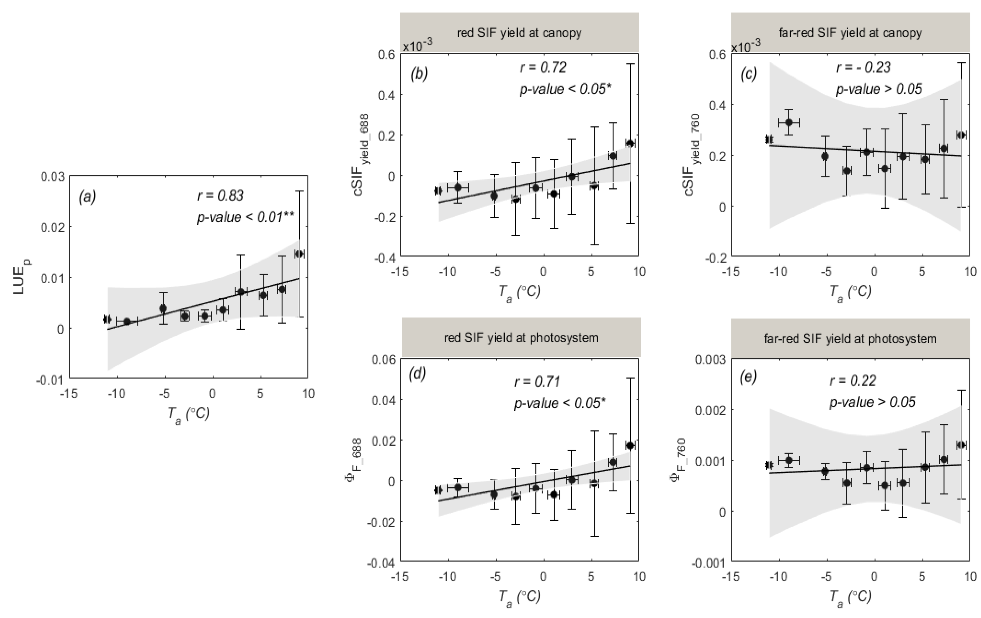
3.2. Temperature Responses of GPP and SIF during Overwintering Period

Firstly, we found that GPP and $cSIF$ both responded to $T_a$ (Figure 6a–c). However, GPP and red SIF ($cSI{F}_{688}$) showed a relatively more obvious change in response to $T_a$ than $cSI{F}_{760}$ did. We can also see that $fPAR$ showed a horizontal trend with $T_a$ with the correlation coefficient (r) of −0.27 (p-value > 0.05, Figure 6g), and$Re{d}_v$ exhibited a significant decreasing trend with increasing $T_a$ (Figure 6e), while $NI{R}_v$ was not sensitive to $T_a$ (Figure 6f). In this study, $f_{esc\_688}$ was estimated by $Re{d}_v/fPAR$, and the changes in $Re{d}_v$ and $fPAR$ could indirectly reflect dynamics in $f_{esc\_688}$ (Figure 6h). Similarly, the $f_{esc\_760}$ was estimated by $NI{R}_v/fPAR$, and the changes in $NI{R}_v$ and $fPAR$ could indirectly reflect dynamics in $f_{esc\_760}$ (Figure 6i). In addition, we found that $cSI{F}_{760}$ was enhanced at about −10 °C (Figure 6c).

We further analyzed how the $LU{E}_p$ and fluorescence quantum yield ($cSI{F}_{yield}$ and ${\mathsf{\Phi }}_F$) changed in response to $T_a$ (Figure 7). From Figure 7a, we can see that $LU{E}_p$ was strongly related to $T_a$ with a high r value of 0.83. This result indicates that photosynthetic activity substantially decreased at low temperatures (Figure 4b). $cSI{F}_{yield\_688}$ and ${\mathsf{\Phi }}_{F\_688}$ were also strongly related to $T_a$ (r = 0.72, 0.71; p-value < 0.05, Figure 7b,d). However, it should be noted that $cSI{F}_{yield\_760}$ and ${\mathsf{\Phi }}_{F\_760}$ exhibited different responses to $T_a$, and the fitted lines were almost invariant (r = −0.23, 0.22; p-value > 0.05). $cSI{F}_{yield\_760}$ and ${\mathsf{\Phi }}_{F\_760}$ at a low temperature (about −10 °C) were greater than that at about 0 °C, which might result in the far-red SIF quantum yields not being sensitive to low temperature. In addition, the $fPAR$ did not correlate with $T_a$ (r = −0.27, p-value > 0.05), which had less impact on the estimation of $cSI{F}_{yield}$ and ${\mathsf{\Phi }}_F$ during the overwintering period.

We also explored the different responses of photosynthesis and fluorescence to $T_a$. From Figure 8, we can see that $\frac{LU{E}_p}{cSI{F}_{yield}}$ (equals to $\frac{GPP}{cSIF}$) and $\frac{LU{E}_p}{{\mathsf{\Phi }}_F}$ (equals to $\frac{GPP}{tSIF}$) were well correlated with $T_a$. This indicates that photosynthesis and fluorescence responded differently to $T_a$. However, it should be noted that the increase in $\frac{LU{E}_p}{cSI{F}_{yield\_688}}$ and $\frac{LU{E}_p}{{\mathsf{\Phi }}_{F\_688}}$ with $T_a$ mainly resulted from the different physiological responses of $LU{E}_p$ and ${\mathsf{\Phi }}_{F688}$ to $T_a$, while the increase in $\frac{LU{E}_p}{cSI{F}_{yield\_760}}$ and $\frac{LU{E}_p}{{\mathsf{\Phi }}_{F\_760}}$ in response to $T_a$ largely contributed to the temperature response of $LU{E}_p$ (Figure 7). These results suggest that SIF-based GPP estimation should consider the effects of temperature.

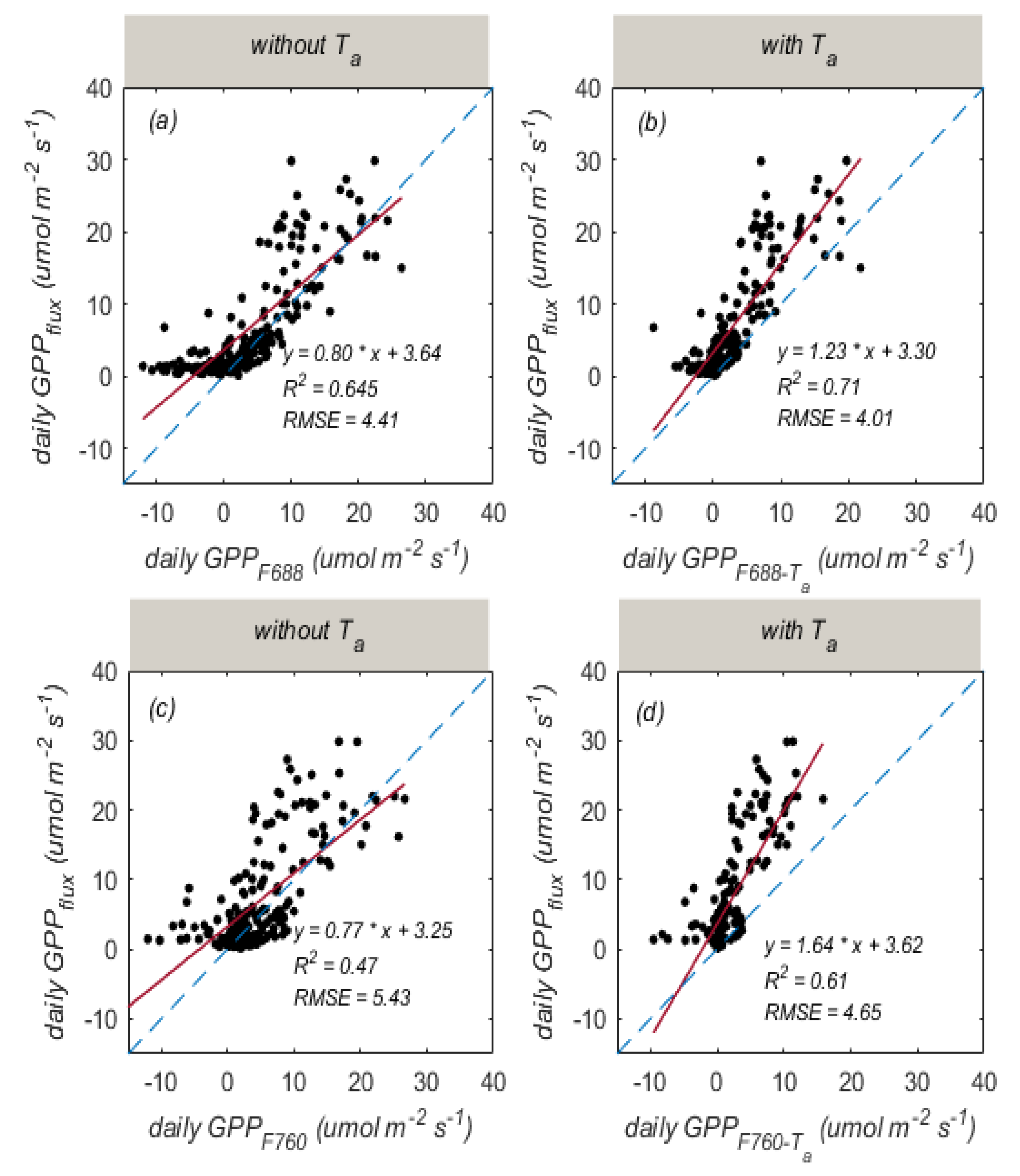
3.3. Improved SIF-Based GPP Estimation by Considering the Influence of Temperature

From Figure 8, we also see that the responses of photosynthesis and fluorescence to temperature were different during the overwintering period. In addition, from Figures S18 and S19, we also found that the sensitivities of SIF and GPP in response to temperature were different during the entire growing season. Therefore, GPP estimation based on SIF should consider the influence of temperature. In this study, we separately analyzed the correlation of GPP with the total red SIF ($tSI{F}_{688}$) and the total far-red SIF ($tSI{F}_{760}$) and explored the effects of temperature on the $tSIF$–GPP relationship during the entire growing season. We compared the relationships between the measured GPP by the EC technique (referred to as $GP{P}_{flux}$ hereafter) and the predicted GPP based on $tSIF$ with or without considering the effects of temperature (

Table 1. The $tSIF$ -based GPP models with and without considering the effects of $T_a$ based on half-hourly and daily mean data. The $f\left(T_a\right)$ is the temperature-corrected function.

Temporal Resolution	Band	Regression Equation	R2	RMSE
half-hourly	688 nm	$GP{P}_{F688}=0.69\times tSI{F}_{688}$	0.64	4.90
		$GP{P}_{F688-T_a}=0.69\times f\left(T_a\right)\times tSI{F}_{688}$	0.69	4.58
	760 nm	$GP{P}_{F760}=9.44\times tSI{F}_{760}$	0.42	6.22
		$GP{P}_{F760-T_a}=9.44\times f\left(T_a\right)\times tSI{F}_{760}$	0.54	5.51
daily	688 nm	$GP{P}_{F688}=0.72\times tSI{F}_{688}$	0.65	4.41
		$GP{P}_{F688-T_a}=0.72\times f\left(T_a\right)\times tSI{F}_{688}$	0.71	4.01
	760 nm	$GP{P}_{F760}=10.2\times tSI{F}_{760}$	0.47	5.43
		$GP{P}_{F760-T_a}=10.2\times f\left(T_a\right)\times tSI{F}_{760}$	0.61	4.65

).

Based on half-hourly data during the entire growing season, we can see that there was a good relationship between $GP{P}_{flux}$ and $GP{P}_{F688}$ (R² = 0.64, RMSE = 4.90 ${\mathrm{umol} \mathrm{CO}}_2{ \mathrm{m}}^{-2}{ \mathrm{s}}^{-1}$), whereas there was a relatively weaker relationship between $GP{P}_{flux}$ and $GP{P}_{F760}$ (R² = 0.42, RMSE = 6.22 ${\mathrm{umol} \mathrm{CO}}_2{ \mathrm{m}}^{-2}{ \mathrm{s}}^{-1}$; Figure 9a,c). The $cSI{F}_{yield\_688}$ and ${\mathsf{\Phi }}_{F\_688}$ exhibited significantly positive correlations with $T_a$ (r > 0.7, p-value < 0.05), while $cSI{F}_{yield\_760}$ and ${\mathsf{\Phi }}_{F\_760}$ were weakly correlated with $T_a$ (r < 0.3, p-value > 0.05; Figure 7). The $tSI{F}_{688}$ explained large variations in GPP while $tSI{F}_{760}$ could explain fewer variations in GPP. Because photosynthesis and fluorescence responded differently to temperature (Figure 8), we further explored the performance of GPP estimation based on $tSIF$ by considering the influence of temperature using a temperature-corrected function. By using the empirical temperature-corrected equation, the GPP estimation based on $tSI{F}_{760}$ was improved (the RMSE dropped from 6.22 to 5.51 ${\mathrm{umol} \mathrm{CO}}_2{ \mathrm{m}}^{-2}{ \mathrm{s}}^{-1}$, while R² values increased from 0.42 to 0.54; Figure 9d). Similar results can also be seen from the $tSI{F}_{688}$–GPP relationship by considering air temperature (the RMSE decreased from 4.90 to 4.58 ${\mathrm{umol} \mathrm{CO}}_2{ \mathrm{m}}^{-2}{ \mathrm{s}}^{-1}$, while R² values increased from 0.64 to 0.69; Figure 9b).

Based on daily mean data during the entire growing season, we can also find that there was a good relationship between $GP{P}_{flux}$ and $GP{P}_{F688}$ (R² = 0.645, RMSE = 4.41 ${\mathrm{umol} \mathrm{CO}}_2{ \mathrm{m}}^{-2}{ \mathrm{s}}^{-1}$), but a relatively weaker relationship between $GP{P}_{flux}$ and $GP{P}_{F760}$ (R² = 0.47, RMSE = 5.43 ${\mathrm{umol} \mathrm{CO}}_2{ \mathrm{m}}^{-2}{ \mathrm{s}}^{-1}$; Figure 10a,c). By considering the influences of $T_a$, $tSI{F}_{760}$-based GPP estimation was improved (RMSE dropped from 5.43 to 4.65 ${\mathrm{umol} \mathrm{CO}}_2{ \mathrm{m}}^{-2}{ \mathrm{s}}^{-1}$, while R² values increased from 0.47 to 0.61; Figure 10d). $tSI{F}_{688}$-GPP estimation was also improved (RMSE decreased from 4.41 to 4.01 ${\mathrm{umol} \mathrm{CO}}_2{ \mathrm{m}}^{-2}{ \mathrm{s}}^{-1}$, while R² values increased from 0.65 to 0.71; Figure 10b) by integrating $T_a$ with $tSI{F}_{688}$. This indicated that considering the effects of temperature could improve the SIF-based GPP estimation at different time scales. Overall, the above results demonstrate that the SIF–GPP models should consider the influence of temperature.

4. Discussion

4.1. Error Sources in Estimation of $cSI{F}_{yield}$ and ${\Phi }_F$

In this study, $cSI{F}_{yield}$ and ${\mathsf{\Phi }}_F$ were calculated based on some assumptions. The $fPAR$ was not measured directly and was generally estimated by spectral indices, such as WDRVI. Although WDRVI is a good proxy of $fPAR$ for different soil backgrounds (Figures S1, S3 and S4), it should be noted that WDRVI cannot represent the impact of direct and diffuse radiation components on $fPAR$. This will bring some uncertainties to the estimation of $cSI{F}_{yield}$.

It is very challenging to accurately retrieve ${\mathsf{\Phi }}_F$ using remote sensing approaches [40]. By investigating the radiative transfer process within the canopy, Yang and van der Tol [51] showed that $f_{esc\_760}$ could be mostly explained by the canopy reflectance, canopy interception probability ($i_0$) and leaf albedo (${\omega }_L$). Zeng et al. [54] used the near-infrared reflectance of vegetation ($NI{R}_v$) and the $fPAR$ to estimate the $f_{esc\_760}$, but this method is not applicable to the red band SIF. Using the random-forest regression method, Liu et al. [41] introduced a practical approach (Random Forest, abbreviated as RF) to estimate the SIF escape probability and further explored a simple NDVI²-corrected method to compensate for the effects of the soil background [21]. It should also be noted that the $Re{d}_v$ is not strictly derived because the mixing of vegetation and soil reflectance at the red band is much more complex than at the NIR band and is influenced by the brightness of the soil and the vegetation’s structural and component parameters. Yang et al. [51] found that the scattered portion of soil does not affect the relationship due to the fact that the scattering of the soil is indifferent to the emitted SIF or scattered incident. However, the part of the soil receiving solar or sky light directly can contribute to the observed reflected flux but not to the observed SIF because it does not produce SIF. The direct contribution of sunlit soil to TOC reflectance may affect the relationship and change with canopy coverage. Based on the SCOPE simulations (Figures S8 and S9), we can see that $f_{esc\_688}$ estimated by $Re{d}_v/fPAR$ agreed moderately well with that estimated by RF. However, the fact that the $Re{d}_v/fPAR$ approach shows a nonlinear, saturating relationship with $f_{esc\_688}$ suggests this approach could introduce misleading trends in $f_{esc\_688}$. These modeling results are yet to be validated with rigorous field measurements. From Figure 5, we can see that $Re{d}_v/fPAR$ and $NI{R}_v/fPAR$ had the same temporal variations, except for April–June. This indicates that different study periods might have an influence on the SIF–GPP relationship (Figure 9 and Figure 10). Therefore, this might indicate that the changes in pigment pool and canopy structure did have some potential influence on the estimation of $f_{esc}$ and ${\mathsf{\Phi }}_F$ and cause some uncertainty regarding the results.

Until now, the accurate estimation of ${\mathsf{\Phi }}_F$ has relied on the accurate estimation of $f_{esc}$, while $f_{esc}$ has largely been influenced by canopy structure, ${\omega }_L$ and the soil background effects. Firstly, the canopy structure in winter wheat changes dramatically during the entire growing period. Due to the effects of low-temperature stress, the canopy structure in winter wheat can also change [31,65]. There might be some uncertainties in the estimation of $f_{esc}$ due to the fact that the soil background would be exposed for too much time during the overwintering period in winter wheat. Secondly, ${\omega }_L$ in the red band is not constant across the growing season, and the temporal variations in leaf pigment content would induce a temporally varying ${\omega }_L$, which could further cause misleading changes in $f_{esc\_688}$. Thirdly, the estimation of $f_{esc\_688}$ by $Re{d}_v/fPAR$ ignored the effects of soil background, despite the fact that $NDV{I}^2$ could be used to correct vegetation reflectance from the apparent reflectance. We conducted sensitivity tests on the estimation of $f_{esc\_688}$ and ${\mathsf{\Phi }}_{F\_688}$ and on their responses to temperature by varying ${\omega }_L$ (Figures S5 and S6). Based on the PROSPECT-D model, we found that ${\omega }_{688}$ was largely influenced by leaf chlorophyll a/b concentration ($C_{ab}$) and exhibited a decreasing trend with increasing $C_{ab}$. Due to the changes in pigment pool affecting the estimation of $f_{esc\_688}$ more than that of $f_{esc\_760}$ (Figures S5 and S6), the responses of ${\mathsf{\Phi }}_{F\_688}$ estimated by $f_{esc\_688}$ to temperature contained some uncertainties resulting from the changes in pigment content. Therefore, we changed $C_{ab}$ in SCOPE model to change the ${\omega }_L$ and further estimated the variations of $f_{esc\_688}$ and ${\mathsf{\Phi }}_{F\_688}$. From Figure S6, we can see that $C_{ab}$ affects $f_{esc\_688}$ and ${\mathsf{\Phi }}_{F\_688}$ estimated by $Re{d}_v$, which indicates that seasonal variations of $C_{ab}$ along with temperature would cause misleading changes in $f_{esc\_688}$ in response to temperature. Many studies have demonstrated that canopy observed SIF and $f_{esc}$ were largely influenced by changes in $C_{ab}$ [15,16,66]. Finally, although the zenith inclination distribution of the leaves in winter wheat is random and the leaf clumping effects in planophile wheat are generally not obvious [67,68,69], we only assessed the above assumptions using the SCOPE model, which assumes that the canopy is horizontally homogenous and has full canopy cover over the soil background; further testing with 3D radiative transfer models will be helpful (e.g., Discrete Anisotropic Radiative Transfer, abbreviated as DART; [70,71]). In addition, it should be noted that the depths of the O₂B are generally smaller than that of O₂A. $cSIF$ retrievals at the O₂B band are generally less robust than those at the O₂A band due to the different absorption depths [41], which might also result in some uncertainties.

4.2. Different Sensitivities of SIF and GPP to Air Temperature

In our study, we explored the changes in SIF and GPP in response to low temperatures in winter wheat. Based on the measurements in the whole growth period (Figure 4), we found that both $cSI{F}_{688}$ and $cSI{F}_{760}$ could track GPP well, and they recorded the reduction in GPP in the overwintering period (Figure 4a,d,g). The results show that low temperature simultaneously inhibited both photosynthesis and fluorescence, which was in accordance with earlier research [8,15]. However, SIF and GPP responded differently to air temperature in this study. From Figure 8, we can see that both $\frac{LU{E}_p}{cSI{F}_{yield}}$ and $\frac{LU{E}_p}{{\mathsf{\Phi }}_F}$ increased with $T_a$, which indicates that the temperature sensitivity of fluorescence and photosynthesis was different. For red band SIF, the increases in $\frac{LU{E}_p}{cSI{F}_{yield\_688}}$ and $\frac{LU{E}_p}{{\mathsf{\Phi }}_{F\_688}}$ with $T_a$ can be attributed to $LU{E}_p$ being more sensitive to temperature than $cSI{F}_{yield\_688}$ and ${\mathsf{\Phi }}_{F\_688}$, although they also responded to air temperatures (Figure 8a,c). For far-red band SIF, the increases in $\frac{LU{E}_p}{cSI{F}_{yield\_760}}$ and $\frac{LU{E}_p}{{\mathsf{\Phi }}_{F\_760}}$ with $T_a$ can largely be interpreted by the response of $LU{E}_p$ to temperature (Figure 4c,e and Figure 7b,d). This study only used a linear model to predict changeable trends of variables and to study the relationships between SIF and GPP and the different responses to temperature (Figure 7 and Figure 8). In the future, a large number of leaf level measurements collaborated with the canopy-level observations should be conducted to better investigate the effects of temperature on the SIF–GPP relationship.

Assuming that temperature responses of canopy-level and photosystem-level SIF represented the true physical processes, the potential factors affecting the different sensitivities of $LU{E}_p$ and $cSI{F}_{yield}$ or ${\mathsf{\Phi }}_F$ in response to air temperature could be due to their different physiological mechanisms [5,6]. Under environmental stress conditions, light reactions might operate on distinct time scales from those that carbon reactions operate on photosynthesis [4,72]. The low temperature in winter generally slows down the activities of the carboxylation process. Thus, $LU{E}_p$, which is related to carbon reactions, would rapidly respond to air temperature. If low-temperature stress persists, plants will further decompose photosynthetic proteins (e.g., LHC). SIF is directly related to light reactions. Thus, the different physiological changes between the light reaction and carbon reaction might be attributed to the different sensitivities of $LU{E}_p$ and $cSI{F}_{yield}$ or ${\mathsf{\Phi }}_F$ in response to temperature.

The absorbed light cannot be completely utilized for CO₂ fixation under low temperatures. If the extra absorbed light cannot be released effectively, it will damage the photochemical tissue. Therefore, NPQ is a crucial photoprotection mechanism to protect PSII from damage caused by cold temperatures and high light [11]. Magney et al. [8] found that SIF tracked GPP well over the course of the overwintering period for evergreen needle forests (ENF) and pointed out that the extra absorbed light can be released by NPQ under chilling. According to Porcar-Castell et al. [6], seasonal fluctuations in leaf-level fluorescence quantum efficiency were found to be in agreement with the quantum yield of photochemistry for ENF over winter [7,8]. In ENF during the fall transition, Kim et al. [15] found that the daily mean $LU{E}_p$ showed saturated phenomena in high air temperatures, but ${\mathsf{\Phi }}_F$ increased gradually with air temperature. NPQ is an important regulated mechanism in the energy distribution, and photochemistry and fluorescence might decrease simultaneously when NPQ increases [6,8]. In addition, SIF is directly linked with electron transport, and electron transport (linear, cyclic, pseudo-cyclic) still operates under cold conditions if there is light available, which is another important photoprotective mechanism [24,73]. The uncertain energy distribution under cold conditions and the potential response of PSI and PSII fluorescence to environmental stress might result in the dynamic range of ${\mathsf{\Phi }}_F$ being smaller than that of $LU{E}_p$ in response to low temperature. In addition, some studies have reported that clear and cloudy conditions can affect the relationship between SIF and GPP [36]. We further evaluated the clear and cloudy conditions on the $tSIF$–GPP relationship by considering $T_a$ (Figures S11 and S12), and the results also showed that the $tSIF$–GPP relationship was affected by $T_a$ during both clear and cloudy days. By removing the negative $tSIF$ values, an improvement in the GPP estimation based on $tSIF$ by considering $T_a$ was also found (Figures S16 and S17). In our study, we found that there were certain different sensitivities in response to air temperature between $LU{E}_p$ and ${\mathsf{\Phi }}_F$, which indicated that the influence of temperature should be considered for a more accurate SIF–GPP model.

4.3. Why Red SIF Tracks GPP Better Than Far-Red SIF under Low Air Temperature

In this study, we found that both daily $LU{E}_p$ and ${\mathsf{\Phi }}_{F\_688}$ were affected by temperature and declined over the overwintering period (Figure 4 and Figure 7), but this was not the case for ${\mathsf{\Phi }}_{F\_760}$. The ${\mathsf{\Phi }}_{F\_760}$ remained almost invariant with $T_a$ (Figure 7d). Therefore, our results confirmed from some aspects that SIF at the red band and far-red band contained different information and showed different abilities to track changes in photosynthesis under environmental stresses [21].

This phenomenon can be attributed to more information about PSII contained in red-band $tSIF$. Photosynthesis has two photosystems. Both photosystems are engaged in the fluorescence spectrum emitted from chloroplasts (Figure 1), which covers a wavelength range of 640–850 nm [74]. However, the fluorescence spectrum emitted from PSII has two peaks, with the amplitude of the left peak (~685 nm) being substantially larger than that of the right peak (~740 nm), whereas the fluorescence spectrum emitted from PSI only has one peak at 740 nm [21,74]. The far-red $tSIF$ thus contains contributions from both PSI and PSII. The relative contribution of PSI fluorescence is normally modest compared to PSII fluorescence, and PSI fluorescence generally remains constant under changeable illumination. However, some studies have reported that the PSI activity is enhanced in response to winter cold for overwintering plants [7,24]. The contribution of PSII $tSIF$ in the red bands is near 100%, which was significantly higher than that in the far-red SIF, in which PSII $tSIF$ contributes only about 50% depending on the measurement conditions [74,75]. Some studies proposed a practical approach to separately estimate the fraction of PSII in the red and far-red regions, and found that the contribution of PSII $tSIF$ was 86% and 55%, respectively [76]. In addition, many studies assumed that the ratio of APAR allocated to PSII is 0.5 when calculating the PSII $tSIF$, but, in fact, the ratio of PSII $tSIF$ changes dynamically [4,8]. PSII: PSI is approximately 2:1 in C3 plants and approximately 1:1 in C4 plants [77]. Variation in the proportion of $tSIF$ between PSI and PSII may affect the generalizability of the $tSIF$–GPP relationship. Gu et al. [4] proposed a photosynthetic mechanism model which quantitatively describes the coupling relationship between GPP and the total SIF of PSII, but there are still a series of problems to be solved in the calculation of the total fluorescence of PSII. Therefore, it is important for the quantitative estimation of GPP to disentangle the dynamic changes in PSI $tSIF$ and PSII $tSIF$, especially under environmental stress conditions.

In addition, due to the large variations in sun-target-viewing geometries, the angular effects play an important role in interpreting directional SIF observed at the canopy level. Some studies have reported that the nadir-adjusted SIF was independent of viewing angle effects and showed a similarly good performance in estimating GPP for both red and far-red bands compared to $tSIF$ [78,79]. The angular effects in canopy observed SIF could bring some uncertainties in estimating GPP. It should be noted that the correlation between $LU{E}_p$ and $f_{esc}$ is the key point to determining the different performances of the nadir-adjust SIF and $tSIF$ in approximating GPP [79]. Although the $tSIF$ eliminates the influences of the angle effects, the estimation of $tSIF$ relies on accurate information about canopy structure parameters [39,80]. Thus, the estimation of canopy-structure parameters using remote-sensing methods will bring some uncertainties in evaluating the $tSIF$–GPP relationship.

In our study, we found that ${\mathsf{\Phi }}_{F\_760}$ exhibited a different pattern in response to low temperature compared to ${\mathsf{\Phi }}_{F\_688}$ (Figure 4f,i). This may be explained by the fact that low temperature inhibited the PSII activity, and the electrons transferred more to the PSI, which could result in the enhancement of the PSI activity, and the magnitude of the $tSIF$ from PSI might also increase. Therefore, the increase in the $tSIF$ from PSI could be compensated for the decline in the $tSIF$ from PSII, especially at the far-red band. However, the PSII portion of the red $tSIF$ might dominate the red SIF, and thus the red SIF quantum yield at the photosystem level (${\mathsf{\Phi }}_{F\_688}$) might be likely to decline in the overwintering period. Goulas et al. [30] explored the apparent spectral fluorescence yields ($ASI{F}_{yield\_687}$ and $ASI{F}_{yield\_760}$, which were measured by SIF normalized with PAR) for wheat in correlation with GPP and found that $cSI{F}_{760}$ related more strongly to GPP than $cSI{F}_{688}$. It should be noted that $cSI{F}_{760}$ carries much information relating to the canopy structure. Goulas et al. [30] only explored the GPP estimation based on canopy SIF. In our study, we used ANCOVA analysis to explore the difference between ${\mathsf{\Phi }}_{F\_688}$ and ${\mathsf{\Phi }}_{F\_760}$ and found that they had a significant difference (p-value < 0.05; Figure S15 and Table S5). Therefore, we could infer that the different changes in ${\mathsf{\Phi }}_{F\_760}$ and ${\mathsf{\Phi }}_{F\_688}$ in response to temperature may result from the SIF at the red band, and the far-red band contains different contributions from both PSI and PSII.

5. Conclusions

In this research, we explored the potential mechanisms linking SIF to GPP in winter wheat over overwintering periods. We found that low temperature simultaneously inhibited both photosynthesis and fluorescence during overwintering periods in winter wheat. In addition, we also found that $LU{E}_p$ was more sensitive to $T_a$ than ${\mathsf{\Phi }}_F$, which caused changes in the $LU{E}_p/{\mathsf{\Phi }}_F$ ratio in response to $T_a$. By considering the influence of $T_a$, the $tSIF$-based GPP estimation was significantly improved (with R² increased by more than 0.12 for $tSI{F}_{760}$ and more than 0.05 for $tSI{F}_{688}$). Therefore, our results show that GPP was more sensitive to temperature than SIF and highlighted that the GPP estimation based on SIF should consider the influence of temperature.

References

1. Schimel, D.S. Terrestrial ecosystems and the carbon cycle. Glob. Chang. Biol. 1995, 1, 77–91. [Google Scholar] [CrossRef]
2. Berry, J.; Wolf, A.; Campbell, J.E.; Baker, I.; Blake, N.; Blake, D.; Denning, A.S.; Kawa, S.R.; Montzka, S.A.; Seibt, U. A coupled model of the global cycles of carbonyl sulfide and CO2: A possible new window on the carbon cycle. J. Geophys. Res. Biogeosci. 2013, 118, 842–852. [Google Scholar] [CrossRef] [Green Version]
3. Frankenberg, C.; O’Dell, C.; Berry, J.; Guanter, L.; Joiner, J.; Köhler, P.; Pollock, R.; Taylor, T.E. Prospects for chlorophyll fluorescence remote sensing from the Orbiting Carbon Observatory-2. Remote Sens. Environ. 2014, 147, 1–12. [Google Scholar] [CrossRef] [Green Version]
4. Gu, L.; Han, J.; Wood, J.D.; Chang, C.Y.Y.; Sun, Y. Sun-induced Chl fluorescence and its importance for biophysical modeling of photosynthesis based on light reactions. New Phytol. 2019, 223, 1179–1191. [Google Scholar] [CrossRef] [PubMed] [Green Version]
5. Baker, N.R. Chlorophyll fluorescence: A probe of photosynthesis in vivo. Annu. Rev. Plant Biol. 2008, 59, 89–113. [Google Scholar] [CrossRef] [PubMed] [Green Version]
6. Porcar-Castell, A.; Tyystjärvi, E.; Atherton, J.; Van der Tol, C.; Flexas, J.; Pfündel, E.E.; Moreno, J.; Frankenberg, C.; Berry, J.A. Linking chlorophyll a fluorescence to photosynthesis for remote sensing applications: Mechanisms and challenges. J. Exp. Bot. 2014, 65, 4065–4095. [Google Scholar] [CrossRef] [PubMed]
7. Li, Y.; Hou, R.; Tao, F. Interactive effects of different warming levels and tillage managements on winter wheat growth, physiological processes, grain yield and quality in the North China Plain. Agric. Ecosyst. Environ. 2020, 295, 106923. [Google Scholar] [CrossRef]
8. Magney, T.S.; Bowling, D.R.; Logan, B.A.; Grossmann, K.; Stutz, J.; Blanken, P.D.; Burns, S.P.; Cheng, R.; Garcia, M.A.; Köhler, P. Mechanistic evidence for tracking the seasonality of photosynthesis with solar-induced fluorescence. Proc. Natl. Acad. Sci. USA 2019, 116, 11640–11645. [Google Scholar] [CrossRef] [Green Version]
9. Russell, R.B.; Lei, T.T.; Nilsen, E.T. Freezing induced leaf movements and their potential implications to early spring carbon gain: Rhododendron maximum as exemplar. Funct. Ecol. 2009, 23, 463–471. [Google Scholar] [CrossRef]
10. Savitch, L.V.; Ivanov, A.G.; Krol, M.; Sprott, D.P.; Öquist, G.; Huner, N.P. Regulation of energy partitioning and alternative electron transport pathways during cold acclimation of lodgepole pine is oxygen dependent. Plant Cell Physiol. 2010, 51, 1555–1570. [Google Scholar] [CrossRef]
11. Verhoeven, A. Sustained energy dissipation in winter evergreens. New Phytol. 2014, 201, 57–65. [Google Scholar] [CrossRef]
12. Li, X.-P.; BjoÈrkman, O.; Shih, C.; Grossman, A.R.; Rosenquist, M.; Jansson, S.; Niyogi, K.K. A pigment-binding protein essential for regulation of photosynthetic light harvesting. Nature 2000, 403, 391–395. [Google Scholar] [CrossRef] [PubMed]
13. Flexas, J.; Medrano, H. Drought-inhibition of photosynthesis in C3 plants: Stomatal and non-stomatal limitations revisited. Ann. Bot. 2002, 89, 183–189. [Google Scholar] [CrossRef] [PubMed] [Green Version]
14. Hughes, N.M. Winter leaf reddening in ‘evergreen’species. New Phytol. 2011, 190, 573–581. [Google Scholar] [CrossRef] [PubMed]
15. Kim, J.; Ryu, Y.; Dechant, B.; Lee, H.; Kim, H.S.; Kornfeld, A.; Berry, J.A. Solar-induced chlorophyll fluorescence is non-linearly related to canopy photosynthesis in a temperate evergreen needleleaf forest during the fall transition. Remote Sens. Environ. 2021, 258, 112362. [Google Scholar] [CrossRef]
16. Dechant, B.; Ryu, Y.; Badgley, G.; Köhler, P.; Rascher, U.; Migliavacca, M.; Zhang, Y.; Tagliabue, G.; Guan, K.; Rossini, M. NIRVP: A robust structural proxy for sun-induced chlorophyll fluorescence and photosynthesis across scales. Remote Sens. Environ. 2022, 268, 112763. [Google Scholar] [CrossRef]
17. Pierrat, Z.; Magney, T.; Parazoo, N.C.; Grossmann, K.; Bowling, D.R.; Seibt, U.; Johnson, B.; Helgason, W.; Barr, A.; Bortnik, J. Diurnal and Seasonal Dynamics of Solar-Induced Chlorophyll Fluorescence, Vegetation Indices, and Gross Primary Productivity in the Boreal Forest. J. Geophys. Res. Biogeosci. 2022, 127, e2021JG006588. [Google Scholar] [CrossRef]
18. Chen, J.; Liu, X.; Liu, L.; Du, S.; Ma, Y. Effects of drought on the relationship between photosynthesis and chlorophyll fluorescence for maize. IEEE J. Sel. Top. Appl. Earth Obs. Remote Sens. 2021, 14, 11148–11161. [Google Scholar] [CrossRef]
19. Liu, X.; Liu, Z.; Liu, L.; Lu, X.; Chen, J.; Du, S.; Zou, C. Modelling the influence of incident radiation on the SIF-based GPP estimation for maize. Agric. For. Meteorol. 2021, 307, 108522. [Google Scholar] [CrossRef]
20. Monteith, J. Solar radiation and productivity in tropical ecosystems. J. Appl. Ecol. 1972, 9, 747–766. [Google Scholar] [CrossRef] [Green Version]
21. Liu, X.; Liu, L.; Hu, J.; Guo, J.; Du, S. Improving the potential of red SIF for estimating GPP by downscaling from the canopy level to the photosystem level. Agric. For. Meteorol. 2020, 281, 107846. [Google Scholar] [CrossRef]
22. Agati, G. Response of the in vivo chlorophyll fluorescence spectrum to environmental factors and laser excitation wavelength. Pure Appl. Opt. J. Eur. Opt. Soc. Part A 1998, 7, 797. [Google Scholar] [CrossRef]
23. Van der Tol, C.; Verhoef, W.; Rosema, A. A model for chlorophyll fluorescence and photosynthesis at leaf scale. Agric. For. Meteorol. 2009, 149, 96–105. [Google Scholar] [CrossRef]
24. Bag, P.; Chukhutsina, V.; Zhang, Z.; Paul, S.; Jansson, S. Direct energy transfer from photosystem II to photosystem I confers winter sustainability in Scots Pine. Nat. Commun. 2020, 11, 1–13. [Google Scholar] [CrossRef]
25. Liu, Z.; Zhao, F.; Liu, X.; Yu, Q.; Wang, Y.; Peng, X.; Cai, H.; Lu, X. Direct estimation of photosynthetic CO2 assimilation from solar-induced chlorophyll fluorescence (SIF). Remote Sens. Environ. 2022, 271, 112893. [Google Scholar] [CrossRef]
26. Palombi, L.; Cecchi, G.; Lognoli, D.; Raimondi, V.; Toci, G.; Agati, G. A retrieval algorithm to evaluate the Photosystem I and Photosystem II spectral contributions to leaf chlorophyll fluorescence at physiological temperatures. Photosynth. Res. 2011, 108, 225–239. [Google Scholar] [CrossRef]
27. Kimm, H.; Guan, K.; Burroughs, C.H.; Peng, B.; Ainsworth, E.A.; Bernacchi, C.J.; Moore, C.E.; Kumagai, E.; Yang, X.; Berry, J.A. Quantifying high-temperature stress on soybean canopy photosynthesis: The unique role of sun-induced chlorophyll fluorescence. Glob. Chang. Biol. 2021, 27, 2403–2415. [Google Scholar] [CrossRef]
28. Song, L.; Guanter, L.; Guan, K.; You, L.; Huete, A.; Ju, W.; Zhang, Y. Satellite sun-induced chlorophyll fluorescence detects early response of winter wheat to heat stress in the Indian Indo-Gangetic Plains. Glob. Chang. Biol. 2018, 24, 4023–4037. [Google Scholar] [CrossRef] [Green Version]
29. Wang, X.; Qiu, B.; Li, W.; Zhang, Q. Impacts of drought and heatwave on the terrestrial ecosystem in China as revealed by satellite solar-induced chlorophyll fluorescence. Sci. Total Environ. 2019, 693, 133627. [Google Scholar] [CrossRef]
30. Goulas, Y.; Fournier, A.; Daumard, F.; Champagne, S.; Ounis, A.; Marloie, O.; Moya, I. Gross primary production of a wheat canopy relates stronger to far red than to red solar-induced chlorophyll fluorescence. Remote Sens. 2017, 9, 97. [Google Scholar] [CrossRef] [Green Version]
31. Dechant, B.; Ryu, Y.; Badgley, G.; Zeng, Y.; Berry, J.A.; Zhang, Y.; Goulas, Y.; Li, Z.; Zhang, Q.; Kang, M. Canopy structure explains the relationship between photosynthesis and sun-induced chlorophyll fluorescence in crops. Remote Sens. Environ. 2020, 241, 111733. [Google Scholar] [CrossRef] [Green Version]
32. Li, Y.-N.; Li, Y.-T.; Ivanov, A.G.; Jiang, W.-L.; Che, X.-K.; Liang, Y.; Zhang, Z.-S.; Zhao, S.-J.; Gao, H.-Y. Defective photosynthetic adaptation mechanism in winter restricts the introduction of overwintering plant to high latitudes. bioRxiv 2019, 613117. [Google Scholar] [CrossRef]
33. Liu, L.; Guan, L.; Liu, X. Directly estimating diurnal changes in GPP for C3 and C4 crops using far-red sun-induced chlorophyll fluorescence. Agric. For. Meteorol. 2017, 232, 1–9. [Google Scholar] [CrossRef]
34. Song, X.-D.; Brus, D.J.; Liu, F.; Li, D.-C.; Zhao, Y.-G.; Yang, J.-L.; Zhang, G.-L. Mapping soil organic carbon content by geographically weighted regression: A case study in the Heihe River Basin, China. Geoderma 2016, 261, 11–22. [Google Scholar] [CrossRef]
35. Du, S.; Liu, L.; Liu, X.; Guo, J.; Hu, J.; Wang, S.; Zhang, Y. SIFSpec: Measuring solar-induced chlorophyll fluorescence observations for remote sensing of photosynthesis. Sensors 2019, 19, 3009. [Google Scholar] [CrossRef] [PubMed] [Green Version]
36. Chen, J.; Liu, X.; Du, S.; Ma, Y.; Liu, L. Integrating sif and clearness index to improve maize GPP estimation using continuous tower-based observations. Sensors 2020, 20, 2493. [Google Scholar] [CrossRef]
37. Liu, S.; Li, X.; Xu, Z.; Che, T.; Xiao, Q.; Ma, M.; Liu, Q.; Jin, R.; Guo, J.; Wang, L. The Heihe Integrated Observatory Network: A basin-scale land surface processes observatory in China. Vadose Zone J. 2018, 17, 1–21. [Google Scholar] [CrossRef]
38. Lasslop, G.; Reichstein, M.; Papale, D.; Richardson, A.D.; Arneth, A.; Barr, A.; Stoy, P.; Wohlfahrt, G. Separation of net ecosystem exchange into assimilation and respiration using a light response curve approach: Critical issues and global evaluation. Glob. Chang. Biol. 2010, 16, 187–208. [Google Scholar] [CrossRef] [Green Version]
39. Rahman, M.M.; Lamb, D.; Stanley, J. The impact of solar illumination angle when using active optical sensing of NDVI to infer fAPAR in a pasture canopy. Agric. For. Meteorol. 2015, 202, 39–43. [Google Scholar] [CrossRef]
40. Gitelson, A.A.; Buschmann, C.; Lichtenthaler, H.K. Leaf chlorophyll fluorescence corrected for re-absorption by means of absorption and reflectance measurements. J. Plant Physiol. 1998, 152, 283–296. [Google Scholar] [CrossRef]
41. Liu, X.; Guanter, L.; Liu, L.; Damm, A.; Malenovský, Z.; Rascher, U.; Peng, D.; Du, S.; Gastellu-Etchegorry, J.-P. Downscaling of solar-induced chlorophyll fluorescence from canopy level to photosystem level using a random forest model. Remote Sens. Environ. 2019, 231, 110772. [Google Scholar] [CrossRef]
42. Gitelson, A.A.; Peng, Y.; Huemmrich, K.F. Relationship between fraction of radiation absorbed by photosynthesizing maize and soybean canopies and NDVI from remotely sensed data taken at close range and from MODIS 250 m resolution data. Remote Sens. Environ. 2014, 147, 108–120. [Google Scholar] [CrossRef] [Green Version]
43. Viña, A.; Gitelson, A.A. New developments in the remote estimation of the fraction of absorbed photosynthetically active radiation in crops. Geophys. Res. Lett. 2005, 32, L17403. [Google Scholar] [CrossRef] [Green Version]
44. Sakamoto, T.; Gitelson, A.A.; Wardlow, B.D.; Verma, S.B.; Suyker, A.E. Estimating daily gross primary production of maize based only on MODIS WDRVI and shortwave radiation data. Remote Sens. Environ. 2011, 115, 3091–3101. [Google Scholar] [CrossRef]
45. Mohammed, G.H.; Colombo, R.; Middleton, E.M.; Rascher, U.; van der Tol, C.; Nedbal, L.; Goulas, Y.; Perez-Priego, O.; Damm, A.; Meroni, M. Remote sensing of solar-induced chlorophyll fluorescence (SIF) in vegetation: 50 years of progress. Remote Sens. Environ. 2019, 231, 111177. [Google Scholar] [CrossRef]
46. Plascyk, J.A.; Gabriel, F.C. The Fraunhofer line discriminator MKII-an airborne instrument for precise and standardized ecological luminescence measurement. IEEE Trans. Instrum. Meas. 1975, 24, 306–313. [Google Scholar] [CrossRef]
47. Maier, S.W.; Günther, K.P.; Stellmes, M. Sun-induced fluorescence: A new tool for precision farming. In Digital Imaging and Spectral Techniques: Applications to Precision Agriculture and Crop Physiology; American Society of Agronomy: Madison, WI, USA, 2004; Volume 66, pp. 207–222. [Google Scholar] [CrossRef]
48. Meroni, M.; Colombo, R. Leaf level detection of solar induced chlorophyll fluorescence by means of a subnanometer resolution spectroradiometer. Remote Sens. Environ. 2006, 103, 438–448. [Google Scholar] [CrossRef]
49. Chang, C.Y.; Guanter, L.; Frankenberg, C.; Köhler, P.; Gu, L.; Magney, T.S.; Grossmann, K.; Sun, Y. Systematic assessment of retrieval methods for canopy far-red solar-induced chlorophyll fluorescence using high-frequency automated field spectroscopy. J. Geophys. Res. Biogeosci. 2020, 125, e2019JG005533. [Google Scholar] [CrossRef]
50. Meroni, M.; Rossini, M.; Guanter, L.; Alonso, L.; Rascher, U.; Colombo, R.; Moreno, J. Remote sensing of solar-induced chlorophyll fluorescence: Review of methods and applications. Remote Sens. Environ. 2009, 113, 2037–2051. [Google Scholar] [CrossRef]
51. Yang, P.; van der Tol, C. Linking canopy scattering of far-red sun-induced chlorophyll fluorescence with reflectance. Remote Sens. Environ. 2018, 209, 456–467. [Google Scholar] [CrossRef]
52. Romero, J.M.; Cordon, G.B.; Lagorio, M.G. Re-absorption and scattering of chlorophyll fluorescence in canopies: A revised approach. Remote Sens. Environ. 2020, 246, 111860. [Google Scholar] [CrossRef]
53. Romero, J.M.; Cordon, G.B.; Lagorio, M.G. Modeling re-absorption of fluorescence from the leaf to the canopy level. Remote Sens. Environ. 2018, 204, 138–146. [Google Scholar] [CrossRef]
54. Zeng, Y.; Badgley, G.; Dechant, B.; Ryu, Y.; Chen, M.; Berry, J.A. A practical approach for estimating the escape ratio of near-infrared solar-induced chlorophyll fluorescence. Remote Sens. Environ. 2019, 232, 111209. [Google Scholar] [CrossRef] [Green Version]
55. Badgley, G.; Field, C.B.; Berry, J.A. Canopy near-infrared reflectance and terrestrial photosynthesis. Sci. Adv. 2017, 3, e1602244. [Google Scholar] [CrossRef] [PubMed] [Green Version]
56. Zhang, Z.; Zhang, Y.; Chen, J.M.; Ju, W.; Migliavacca, M.; El-Madany, T.S. Sensitivity of estimated total canopy SIF emission to remotely sensed LAI and BRDF products. J. Remote Sens. 2021, 2021, 9795837. [Google Scholar] [CrossRef]
57. Alexander, M. Introduction to soil microbiology. Soil Sci. 1978, 125, 331. [Google Scholar] [CrossRef]
58. Atlas, R.M.; Bartha, R. Microbial Ecology: Fundamentals and Applications; The Benjamin/Cummings Punlishing: Redwood City, CA, USA, 1993. [Google Scholar]
59. Collins, M.E.; Kuehl, R. Organic matter accumulation and organic soils. In Wetland Soils, Genesis, Hydrology, Landscapes, and Classification; Lewis Pub.: Boca Raton, FL, USA, 2001; pp. 137–162. [Google Scholar]
60. Rabenhorst, M.C. Biologic zero: A soil temperature concept. Wetlands 2005, 25, 616–621. [Google Scholar] [CrossRef]
61. Hao, Z.; Geng, X.; Wang, F.; Zheng, J. Impacts of climate change on agrometeorological indices at winter wheat overwintering stage in Northern China during 2021–2050. Int. J. Climatol. 2018, 38, 5576–5588. [Google Scholar] [CrossRef]
62. Pei, Y.; Dong, J.; Zhang, Y.; Yuan, W.; Doughty, R.; Yang, J.; Zhou, D.; Zhang, L.; Xiao, X. Evolution of light use efficiency models: Improvement, uncertainties, and implications. Agric. For. Meteorol. 2022, 317, 108905. [Google Scholar] [CrossRef]
63. Yuan, W.; Liu, S.; Yu, G.; Bonnefond, J.-M.; Chen, J.; Davis, K.; Desai, A.R.; Goldstein, A.H.; Gianelle, D.; Rossi, F. Global estimates of evapotranspiration and gross primary production based on MODIS and global meteorology data. Remote Sens. Environ. 2010, 114, 1416–1431. [Google Scholar] [CrossRef] [Green Version]
64. Running, S.W.; Nemani, R.R.; Heinsch, F.A.; Zhao, M.; Reeves, M.; Hashimoto, H. A continuous satellite-derived measure of global terrestrial primary production. Bioscience 2004, 54, 547–560. [Google Scholar] [CrossRef]
65. Wood, J.D.; Griffis, T.J.; Baker, J.M.; Frankenberg, C.; Verma, M.; Yuen, K. Multiscale analyses of solar-induced florescence and gross primary production. Geophys. Res. Lett. 2017, 44, 533–541. [Google Scholar] [CrossRef]
66. Koffi, E.; Rayner, P.; Norton, A.; Frankenberg, C.; Scholze, M. Investigating the usefulness of satellite-derived fluorescence data in inferring gross primary productivity within the carbon cycle data assimilation system. Biogeosciences 2015, 12, 4067–4084. [Google Scholar] [CrossRef] [Green Version]
67. Drews, S.; Neuhoff, D.; Köpke, U. Weed suppression ability of three winter wheat varieties at different row spacing under organic farming conditions. Weed Res. 2009, 49, 526–533. [Google Scholar] [CrossRef]
68. Van der Tol, C.; Verhoef, W.; Timmermans, J.; Verhoef, A.; Su, Z. An integrated model of soil-canopy spectral radiances, photosynthesis, fluorescence, temperature and energy balance. Biogeosciences 2009, 6, 3109–3129. [Google Scholar] [CrossRef] [Green Version]
69. Verrelst, J.; van der Tol, C.; Magnani, F.; Sabater, N.; Rivera, J.P.; Mohammed, G.; Moreno, J. Evaluating the predictive power of sun-induced chlorophyll fluorescence to estimate net photosynthesis of vegetation canopies: A SCOPE modeling study. Remote Sens. Environ. 2016, 176, 139–151. [Google Scholar] [CrossRef]
70. Gastellu-Etchegorry, J.-P.; Lauret, N.; Yin, T.; Landier, L.; Kallel, A.; Malenovský, Z.; Al Bitar, A.; Aval, J.; Benhmida, S.; Qi, J. DART: Recent advances in remote sensing data modeling with atmosphere, polarization, and chlorophyll fluorescence. IEEE J. Sel. Top. Appl. Earth Obs. Remote Sens. 2017, 10, 2640–2649. [Google Scholar] [CrossRef]
71. Gastellu-Etchegorry, J.-P.; Yin, T.; Lauret, N.; Cajgfinger, T.; Gregoire, T.; Grau, E.; Feret, J.-B.; Lopes, M.; Guilleux, J.; Dedieu, G. Discrete anisotropic radiative transfer (DART 5) for modeling airborne and satellite spectroradiometer and LIDAR acquisitions of natural and urban landscapes. Remote Sens. 2015, 7, 1667–1701. [Google Scholar] [CrossRef] [Green Version]
72. Pietrini, F.; Chaudhuri, D.; Thapliyal, A.; Massacci, A. Analysis of chlorophyll fluorescence transients in mandarin leaves during a photo-oxidative cold shock and recovery. Agric. Ecosyst. Environ. 2005, 106, 189–198. [Google Scholar] [CrossRef]
73. Ivanov, A.; Sane, P.; Zeinalov, Y.; Malmberg, G.; Gardeström, P.; Huner, N.; Öquist, G. Photosynthetic electron transport adjustments in overwintering Scots pine (Pinus sylvestris L.). Planta 2001, 213, 575–585. [Google Scholar] [CrossRef]
74. Franck, F.; Juneau, P.; Popovic, R. Resolution of the photosystem I and photosystem II contributions to chlorophyll fluorescence of intact leaves at room temperature. Biochim. Biophys. Acta BBA-Bioenerg. 2002, 1556, 239–246. [Google Scholar] [CrossRef] [Green Version]
75. Pfündel, E.E.; Klughammer, C.; Meister, A.; Cerovic, Z.G. Deriving fluorometer-specific values of relative PSI fluorescence intensity from quenching of F 0 fluorescence in leaves of Arabidopsis thaliana and Zea mays. Photosynth. Res. 2013, 114, 189–206. [Google Scholar] [CrossRef]
76. Pfündel, E.E. Simultaneously measuring pulse-amplitude-modulated (PAM) chlorophyll fluorescence of leaves at wavelengths shorter and longer than 700 nm. Photosynth. Res. 2021, 147, 345–358. [Google Scholar] [CrossRef] [PubMed]
77. Peterson, R.B.; Oja, V.; Eichelmann, H.; Bichele, I.; Dall’Osto, L.; Laisk, A. Fluorescence F 0 of photosystems II and I in developing C3 and C4 leaves, and implications on regulation of excitation balance. Photosynth. Res. 2014, 122, 41–56. [Google Scholar] [CrossRef]
78. Zhang, Z.; Zhang, Y.; Zhang, Q.; Chen, J.M.; Porcar-Castell, A.; Guanter, L.; Wu, Y.; Zhang, X.; Wang, H.; Ding, D. Assessing bi-directional effects on the diurnal cycle of measured solar-induced chlorophyll fluorescence in crop canopies. Agric. For. Meteorol. 2020, 295, 108147. [Google Scholar] [CrossRef]
79. Hao, D.; Zeng, Y.; Zhang, Z.; Zhang, Y.; Qiu, H.; Biriukova, K.; Celesti, M.; Rossini, M.; Zhu, P.; Asrar, G.R. Adjusting solar-induced fluorescence to nadir-viewing provides a better proxy for GPP. ISPRS J. Photogramm. Remote Sens. 2022, 186, 157–169. [Google Scholar] [CrossRef]
80. Hao, D.; Zeng, Y.; Qiu, H.; Biriukova, K.; Celesti, M.; Migliavacca, M.; Rossini, M.; Asrar, G.R.; Chen, M. Practical approaches for normalizing directional solar-induced fluorescence to a standard viewing geometry. Remote Sens. Environ. 2021, 255, 112171. [Google Scholar] [CrossRef]
Figure 1. Sample reabsorption and scattering inside leaves (a) and canopy (c). PAR is the photosynthetically active radiation. SIF is the solar-induced chlorophyll fluorescence. R represents the reflectance, and T is the transmittance. A represents the absorbed effects and E indicates the canopy scattering effects. Relative PSII or PSI fluorescence represents the relative magnitude of fluorescence emitted from PSII or PSI, respectively (b).
Remotesensing 14 03076 g001
Figure 2. Details about the XTS site. (a) Location of the XTS farm; (b) Landsat8 image of the XTS farm (the blue dotted line) on 3 August 2020. The location of the XTS tower is represented by the red rectangle, and the location of the eddy covariance system is represented by the orange circle; (c) the spectral measurement system and the approximate field of view (FOV, 25°) represented by the white ellipse.
Remotesensing 14 03076 g002
Figure 3. Seasonal variations in daily mean air temperature ( T a , (a)) The red dotted line in Panel (a) represents the biological zero. The seasonal changes of the photosynthetically active radiation ( P A R , (b)). The shadow represents the overwintering period. Local regression was used to smooth the data. The 95 percent confidence interval is indicated by the black shaded area.
Remotesensing 14 03076 g003
Figure 4. Seasonal dynamics of daily mean G P P (a), L U E p (b) and A P A R (c) are represented in the first row. The second row indicates the changes in canopy c S I F 688 (d), c S I F y i e l d _ 688 (e), and Φ F _ 688 (f). The last row represents the temporal patterns of canopy c S I F 760 (g), c S I F y i e l d _ 760 (h), and Φ F _ 760 (i). The blue shaded rectangle represents the overwintering period. Local regression was used to smooth the data. The black shaded area indicates the 95% confidence interval.
Remotesensing 14 03076 g004
Figure 5. Seasonal dynamics of daily mean f e s c _ 688 (a) and f e s c _ 760 (b). The blue shaded rectangle represents the overwintering periods. Local regression was used to smooth the data. The black shaded area indicates the 95% confidence interval.
Remotesensing 14 03076 g005
Figure 6. The relationships of daily mean G P P (a), c S I F 688 (b), c S I F 760 (c), WDRVI (d), R e d v (e), N I R v (f), f P A R (g), f e s c _ 688 (h), and f e s c _ 760 (i) with air temperature ( T a ). The data were averaged over intervals of 2 °C, and the error bars indicate the standard deviation. The 95% confidence levels for prediction are represented by the grey-shaded zones. * represents a significance level of 0.05 and ** represents a significance level of 0.01.
Remotesensing 14 03076 g006
Figure 7. The relationships of daily mean L U E p (a), c S I F y i e l d _ 688 (b), c S I F y i e l d _ 760 (c), Φ F _ 688 (d), and Φ F _ 760 (e) with air temperature ( T a ). The data were averaged over intervals of 2 °C, and the error bars indicate the standard deviation. The 95% confidence levels for prediction are represented by the grey-shaded zones. * represents a significance level of 0.05 and ** represents a significance level of 0.01.
Remotesensing 14 03076 g007
Figure 8. The relationships of daily mean L U E p / c S I F y i e l d _ 688 (a), L U E p / c S I F y i e l d _ 760 (b), L U E p / Φ F _ 688 (c), and L U E p / Φ F _ 760 (d) with air temperature ( T a ). The data were averaged over intervals of 2 °C, and the error bars indicate the standard deviation. The 95% confidence levels for prediction are represented by the grey-shaded zones. * represents a significance level of 0.05.
Remotesensing 14 03076 g008
Figure 9. The relationships of GPP with t S I F 688 (a), t S I F 688 f ( T a ) (b), t S I F 760 (c), and t S I F 760 f ( T a ) (d) based on half-hour measurements. The blue dotted line is the 1:1 line. The red line is the fitted line.
Remotesensing 14 03076 g009
Figure 10. The relationships of GPP with t S I F 688 (a), t S I F 688 f ( T a ) (b), t S I F 760 (c), and t S I F 760 f ( T a ) (d) based on daily mean data. The blue dotted line is the 1:1 line. The red line is the fitted line.
Remotesensing 14 03076 g010