Low-Complexity 2D DOA Estimation and Self-Calibration for Uniform Rectangle Array with Gain-Phase Error

Abstract

Most subspace-based algorithms need exact array manifold for direction of arrival (DOA) estimation, while, in practical applications, the gain-phases of different array elements are usually inconsistent, degrading their estimation performance. In this paper, a novel low-complexity 2D DOA and gain-phase error estimation algorithm is proposed by adding auxiliary array elements in a uniform rectangular array (URA). Firstly, the URA is modeled as the Kronecker product of two uniform linear arrays (ULAs) to decouple the 2D DOA estimation. Then, several well-calibrated auxiliary array elements are added in the two ULAs, based on which the rotation invariant factor of the URA destroyed by the gain-phase error is reconstructed by solving constrained optimization problems. Lastly, ESPRIT is used to estimate the 2-D DOA and the gain-phase error coefficients. The closed-form expressions of the estimation CRBs are also derived, providing insight into the impact of gain-phase error on DOA estimation. Simulation results are used to validate the effectiveness of the proposed algorithm and the correctness of the theoretical analysis.

1. Introduction

In the research field of array signal processing, direction of arrival (DOA) estimation [1,2,3] has occupied a fundamental position in radar, sonar, and communication systems. At present, many DOA estimation algorithms have been proposed in the one-dimensional (1D) spatial domain, while most arrays in actual systems are rectangular planar arrays. Therefore, study on the two-dimensional (2D) DOA estimation is obviously more meaningful. Many algorithms have been used to estimate the 2D DOAs for uniform rectangle array (URA) [4,5,6], while the effectiveness of these algorithms depends on the precisely known array manifold. In practice, there are inherent unknown antenna array errors, inevitably disturbing the array manifold. If not considered, the performance of these 2D DOA estimation algorithms will be seriously deteriorated [7,8].

According to their different influences on received signals, array errors can be summarized into three categories: mutual coupling, gain-phase error, and position error. Compared with the other two kinds of array errors, gain-phase error is more common in practice. For the calibration of gain-phase error, the algorithms proposed in the early stage require one or several well-calibrated sources as the prior information [9,10]. In order to realize the self-calibration of gain-phase error without well-calibrated sources, a gain-phase blind calibration method was proposed for a linear array with non-Gaussian sources in [11], where the independent component analysis is used to estimate the product of the array error matrix and the array response matrix. By exploiting the ESPRIT algorithm, an approach for DOA and gain-phase estimation was proposed in [12], where the unknown DOAs and gain-phases can be estimated in the closed form without performing a spectral search. Based on a central symmetric array (CSA), the problem of DOA estimation for noncircular sources in the presence of sensor gain-phase uncertainties was studied in [13]. Then, the mixed far-field and near-field source localization was concerned in [14] with the CSA under the condition of gain-phase perturbations. A DOA estimation method based on the errors-in-variables model, i.e., the simultaneous orthogonal matching pursuit-total least squares algorithm, was proposed in [15], where the sparsity of the received signal is exploited. By using the sparse representation technique, an optimization method for direction finding with unknown gain-phase in the presence of spatially non-uniform noise was proposed in [16]. However, all the algorithms mentioned above are proposed for linear arrays and cannot be easily extended to 2D DOA estimation for planar arrays.

To realize 2D DOA estimation in the presence of gain-phase error, a gain-phase calibration algorithm based on subspace was proposed for 2D array in [17]. A simple and robust least-squares algorithm for joint 2D DOA estimation and phase calibration was presented in [18] for URA, while the phase and DOA parameters cannot be identified together without ambiguity when performing phase autocalibration. In study [19], an efficient three-step-iteration algorithm was performed to provide a robust DOA estimator for large URAs in underwater sonar imaging systems. Without the need of good initial guesses, a MUSIC-like iterative calibration algorithm, which uses the improved 2D MUSIC algorithm, was proposed in [20] for the planar equispaced array (PEA). In study [21], by exploiting one well-calibrated incident signal, the 2D DOA and gain-phase error were estimated via the mixing matrix obtained by blind signal separation for a large-scale planar array. Although 2D DOA estimation can be achieved in the presence of gain-phase error, most of the above algorithms need to perform spectral peak search or iterative operation, increasing their computational complexities.

In this study, a novel low-complexity algorithm for 2D DOA and gain-phase error estimation is proposed for URA. The URA is modeled as the Kronecker product of two uniform linear arrays (ULAs) and several well-calibrated auxiliary elements are added into the two ULAs, respectively. Then, the rotation invariances destroyed by the gain-phase error are reconstructed by solving two constrained optimization problems, so that the ESPRIT algorithm can be used for 2D DOA estimation. During the 2D DOA estimation process, the proposed algorithm does not need any gain-phase error information of the URA and can realize the unambiguous joint 2D DOA and gain-phase error coefficient estimation without spectral peak search or iteration operation. Thus, the proposed algorithm has low computational complexity.

Notation:$\otimes$, ⊙, and ◦ denote Kronecker product, Hadamard product, and Khatri-Rao product, respectively. diag[∙] denotes the diagonal matrix formed by a column or row vector, vecd[∙] denotes the column vector formed by the diagonal elements of a matrix. trace[∙] denotes the trace of a matrix. Re(∙) denotes the real part of a plural. arccos[∙] denotes the inverse cosine. E[∙] denotes the expected value. $\left|\right|\cdot |{|}_F$ denotes the Frobenius norm. $\lceil \cdot \rceil$ denotes the ceiling function. (∙)*, (∙)^T, (∙)^H, (∙)⁻¹, and (∙)^# denote complex conjugate, transpose, Hermitian transpose, matrix inverse, and pseudo-inverse, respectively. I_a denotes an a × a identity matrix. 0_a×b denotes an a × b zero matrix.

2. Signal Model of URA with Gain-Phase Error

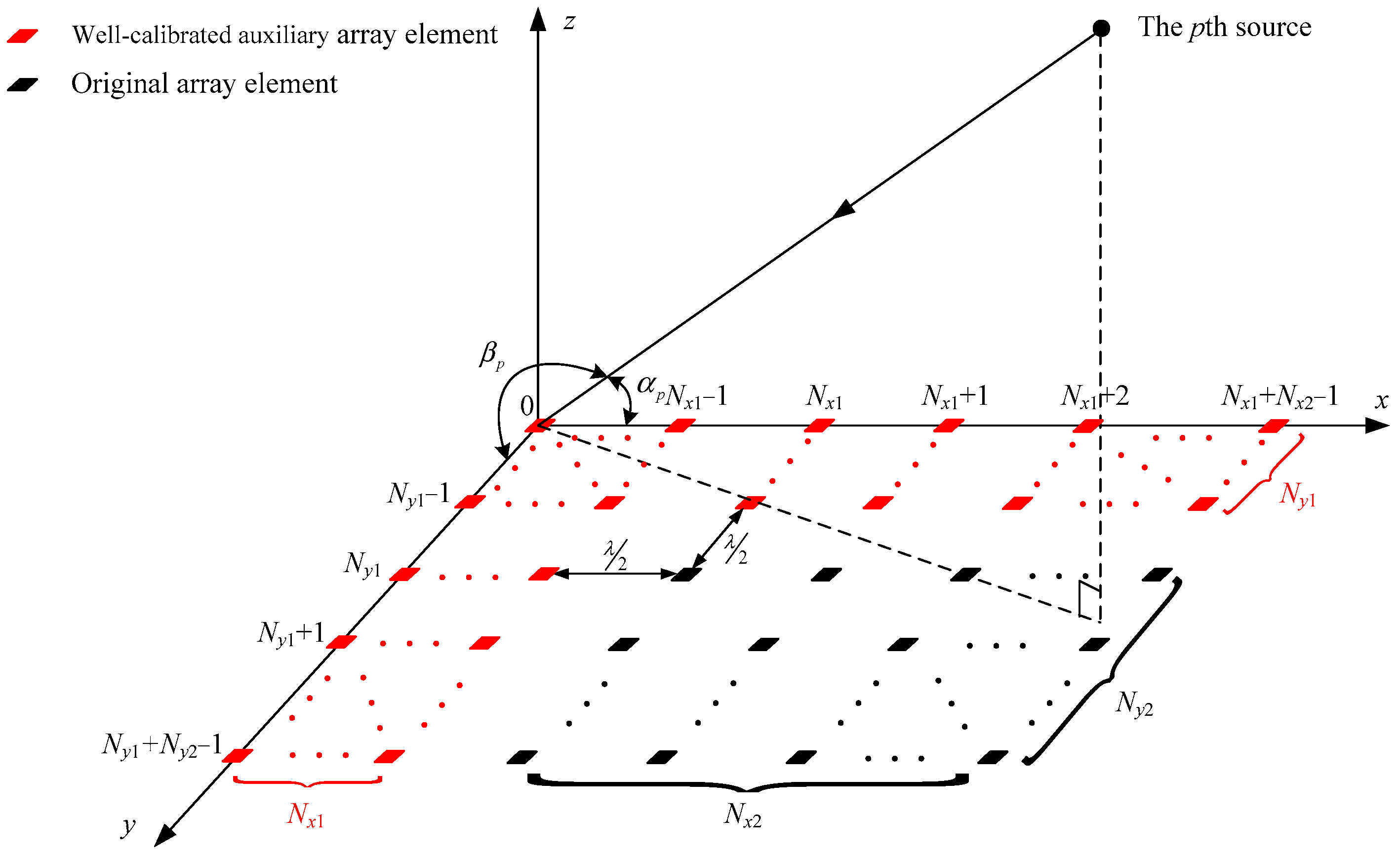
As shown in Figure 1, consider that a URA is located on the x-y plane with N_x2 × N_y2 elements and the distance between the adjacent elements is λ/2, where N_x2 and N_y2 denote the number of array elements along x-axis and y-axis, and λ is wavelength of the received signal. To tackle with the problem of gain-phase error, some well-calibrated auxiliary array elements are added to the URA. The distance between the adjacent auxiliary array elements and the distance between the original URA and the auxiliary array are both λ/2. The position of the (m, n)-th array element is (m, n) × λ/2 with $0\le m\le N_x-1$, $0\le n\le N_y-1$, $N_x=N_{x1}+N_{x2}$, and $N_y=N_{y1}+N_{y2}$. For convenience, we use the auxiliary array element located at (0, 0) as the reference.

Assume that there are P noncoherent far-field sources located at the same range and the 2D DOA of the p-th source with respect to the x-axis and the y-axis are ${\alpha }_p$ and ${\beta }_p$. Then, the received signal of the original URA can be expressed as

$$x\left(t\right)={[x_{N_{x1}{N}_{y1}},x_{\left(N_{x1}+1\right)N_{y1}},\cdots ,x_{\left(N_x-1\right)N_{y1}},\cdots ,x_{N_{x1}\left(N_y-1\right)},\cdots ,x_{\left(N_x-1\right)\left(N_y-1\right)}]}^{\mathrm{T}}={\displaystyle \sum _{p=1}^P\tilde{\Gamma }\tilde{a}\left({\alpha }_p,{\beta }_p\right)s_p\left(t\right)}+\tilde{n}\left(t\right)$$

(1)

where x_mn denotes the received signal of the (m, n)-th array element, $s_p\left(t\right)$ is amplitude of the p-th source, $\tilde{n}\left(t\right)\in {ℂ}^{N_{x2}{N}_{y2}\times 1}$ denotes the noise vector, modeled as a zero-mean spatially white Gaussian noise with the covariance matrix of ${\sigma }_n^2{I}_{N_{x2}{N}_{y2}}$. $\tilde{\Gamma }=\mathrm{diag}\{g_{N_{x1}{N}_{y1}}{e}^{j{\varphi }_{N_{x1}{N}_{y1}}},\cdots ,g_{\left(N_x-1\right)\left(N_y-1\right)}{e}^{j{\varphi }_{\left(N_x-1\right)\left(N_y-1\right)}}\}\in {ℂ}^{N_{x2}{N}_{y2}\times N_{x2}{N}_{y2}}$ is the gain-phase error matrix, g_mn and ${\varphi }_{mn}$ denote the gain and phase error of the (m, n)-th array element, and $\tilde{a}\left({\alpha }_p,{\beta }_p\right)\in {ℂ}^{N_{x2}{N}_{y2}\times 1}$ is the steering vector of the original URA corresponding to the p-th source, described as $\tilde{a}\left({\alpha }_p,{\beta }_p\right)={\tilde{a}}_y\left({\beta }_p\right)\otimes {\tilde{a}}_x\left({\alpha }_p\right)$. It can be seen that the URA can be modeled as the Kronecker product of two ULAs located on the x-axis and y-axis, and thus the 2D DOA can be decoupled.

Similar to Equation (1), the received signal of the extended URA can be expressed as

$$y\left(t\right)={\displaystyle \sum _{p=1}^P\Gamma a\left({\alpha }_p,{\beta }_p\right)s_p\left(t\right)}+n\left(t\right)$$

(2)

where $\Gamma =\mathrm{diag}\{\underset{N_x\times N_{y1}}{\underbrace{1,1,\cdots ,1,}}\underset{N_{x1}}{\underbrace{1,1,\cdots ,1,}}{g}_{N_{x1}{N}_{y1}}{e}^{j{\varphi }_{N_{x1}{N}_{y1}}},\cdots g_{\left(N_x-1\right)N_{y1}}{e}^{j{\varphi }_{\left(N_x-1\right)N_{y1}}},\cdots ,\underset{N_{x1}}{\underbrace{1,1,\cdots ,1,}}{g}_{N_{x1}\left(N_y-1\right)}{e}^{j{\varphi }_{N_{x1}\left(N_y-1\right)}}$, $\cdots ,g_{\left(N_x-1\right)\left(N_y-1\right)}{e}^{j{\varphi }_{\left(N_x-1\right)\left(N_y-1\right)}}\}\in {ℂ}^{N_x{N}_y\times N_x{N}_y}$, $a\left({\alpha }_p,{\beta }_p\right)=a_y\left({\beta }_p\right)\otimes a_x\left({\alpha }_p\right)\in {ℂ}^{N_x{N}_y\times 1}$ is the steering vector of the extended URA corresponding to the pth source with $a_y({\beta }_p)={[1,e^{-j\pi \cos {\beta }_p},\cdots ,e^{-j\pi \left(N_y-1\right)\cos {\beta }_p}]}^{\mathrm{T}}$ and $a_x({\alpha }_p)={[1,e^{-j\pi \cos {\alpha }_p},\cdots ,e^{-j\pi \left(N_x-1\right)\cos {\alpha }_p}]}^{\mathrm{T}}$.

Equation (2) can be rewritten in the matrix form as

$$y\left(t\right)=\Gamma \left(A_y\circ A_x\right)S\left(t\right)+n\left(t\right)=\Gamma AS\left(t\right)+n\left(t\right)$$

(3)

where $A=A_y\circ A_x=[a_y\left({\beta }_1\right)\otimes a_x\left({\alpha }_1\right),a_y\left({\beta }_2\right)\otimes a_x\left({\alpha }_2\right),\cdots ,a_y\left({\beta }_P\right)\otimes a_x\left({\alpha }_P\right)]$, $A_y=[a_y\left({\beta }_1\right), a_y\left({\beta }_2\right),\cdots ,a_y\left({\beta }_P\right)]$, $A_x=\left[a_x\left({\alpha }_1\right),a_x\left({\alpha }_2\right),\cdots ,a_x\left({\alpha }_P\right)\right]$, $S\left(t\right)={\left[s_1\left(t\right),s_2\left(t\right),\cdots ,s_P\left(t\right)\right]}^{\mathrm{T}}$ is the source amplitude vector and $n\left(t\right)\in {ℂ}^{N_x{N}_y\times 1}$ is the zero-mean spatially white Gaussian noise vector of the extended URA with the covariance matrix of ${\sigma }_n^2{I}_{N_x{N}_y}$.

The covariance matrix of y(t) can be expressed as

$$R_y=\mathrm{E}\left[y\left(t\right)y^{\mathrm{H}}\left(t\right)\right]=\Gamma A{R}_S{A}^{\mathrm{H}}{\Gamma }^{\mathrm{H}}+{\sigma }^2{I}_{N_x{N}_y}$$

(4)

By conducting eigenvalue decomposition of $R_y$, the signal subspace $U_s$ and the noise subspace $U_n$ can be obtained. Since the signal subspace U_s and the steering matrix $\Gamma A$ span the same subspace, they have the following relationship

$$U_s=\Gamma AT$$

(5)

where T is a nonsingular matrix.

In the case with finite snapshots, the covariance matrix of y(t) can be estimated by

$${\widehat{R}}_y=\frac{1}{L}{\displaystyle \sum _{l=1}^{L}y\left(t_l\right)y^{\mathrm{H}}\left(t_l\right)}={\widehat{U}}_s{\widehat{\Lambda }}_s{\widehat{U}}_s^{\mathrm{H}}+{\widehat{U}}_n{\widehat{\Lambda }}_n{\widehat{U}}_n^{\mathrm{H}},$$

(6)

3. The Proposed Algorithm

3.1. Algorithm Description

Define the following selective matrix

$$\{\begin{array}{l}{F}_{x1}=I_{N_y}\otimes J_{x1},F_{x2}=I_{N_y}\otimes J_{x2}\\ F_{y1}=J_{y1}\otimes I_{N_x},F_{y2}=J_{y2}\otimes I_{N_x}\end{array},$$

(7)

where J_x1 and J_x2 are the (N_x-1)×N_x submatrices formed by the first and the last N_x-1 rows and $I_{N_x}$, J_y1, and J_y2 are the (N_y-1)×N_y submatrices formed by the first and the last N_y-1 rows of $I_{N_y}$.

Assume $A_{x1}=F_{x1}A=[a_y\left({\beta }_1\right)\otimes a_{x1}\left({\alpha }_1\right),a_y\left({\beta }_2\right)\otimes a_{x1}\left({\alpha }_2\right),\cdots ,a_y\left({\beta }_P\right)\otimes a_{x1}\left({\alpha }_P\right)]$, $A_{x2}=F_{x2}A= [a_y\left({\beta }_1\right)\otimes a_{x2}\left({\alpha }_1\right),a_y\left({\beta }_2\right)\otimes a_{x2}\left({\alpha }_2\right),\cdots ,a_y\left({\beta }_P\right)\otimes a_{x2}\left({\alpha }_P\right)]$, $A_{y1}=F_{y1}A=[a_{y1}\left({\beta }_1\right)\otimes a_x\left({\alpha }_1\right)$, $a_{y1}\left({\beta }_2\right)\otimes a_x\left({\alpha }_2\right),\cdots ,a_{y1}\left({\beta }_P\right)\otimes a_x\left({\alpha }_P\right)]$, $A_{y2}=F_{y2}A=[a_{y2}\left({\beta }_1\right)\otimes a_x\left({\alpha }_1\right),a_{y2}\left({\beta }_2\right)\otimes a_x\left({\alpha }_2\right),\cdots$, $a_{y2}\left({\beta }_P\right)\otimes a_x\left({\alpha }_P\right)]$, where a_x1 and a_x2 are the first and the last N_x-1 elements of a_x; a_y1 and a_y2 are the first and the last N_y-1 elements of a_y. According to the signal model given in Equation (3), the ESPRIT algorithm cannot be directly used to estimate the 2D DOA due to the existence of gain-phase error, while the following proposition makes it possible to reconstruct the rotation invariances of the URA destroyed by the gain-phase error.

Proposition 1. 

Let U_x1, U_x2and U_y1, U_y2be the submatrices formed from U_s in the same way with A_x1, A_x2and A_y1, A_y2formed from A; the extended URA have the following rotation invariances along the x-axis and y-axis

$${\Gamma }_{x12}{U}_{x2}=U_{x1}{T}^{-1}{\Phi }_{x}T=U_{x1}{\Psi }_x,$$

(8a)

$${\Gamma }_{y12}{U}_{y2}=U_{y1}{T}^{-1}{\Phi }_{y}T=U_{y1}{\Psi }_y,$$

(8b)

where ${\Gamma }_{x12}={\Gamma }_{x1}{\Gamma }_{x2}^{-1}$, ${\Gamma }_{x1}$ is a $\left(N_x-1\right)N_y\times \left(N_x-1\right)N_y$ diagonal matrix formed by the diagonal elements of $\Gamma$ without $\Gamma \left(m,m\right),m=1,N_x+1,2N_x+1,\cdots ,\left(N_y-1\right)N_x+1$, ${\Gamma }_{x2}$ is a $\left(N_x-1\right)N_y\times \left(N_x-1\right)N_y$ diagonal matrix formed by the diagonal elements of $\Gamma$ without $\Gamma \left(m,m\right),m=N_x,2N_x,\cdots ,$ $N_y{N}_x$; ${\Gamma }_{y12}={\Gamma }_{y1}{\Gamma }_{y2}^{-1}$, ${\Gamma }_{y1}$ is a $\left(N_y-1\right)N_x\times \left(N_y-1\right)N_x$ diagonal matrix formed by the diagonal elements of $\Gamma$ without $\Gamma \left(m,m\right),m=1,2,\cdots ,N_x$, ${\Gamma }_{y2}$ is a $\left(N_y-1\right)N_x\times \left(N_y-1\right)N_x$ diagonal matrix formed by the diagonal elements of $\Gamma$ without $\Gamma \left(m,m\right),m=\left(N_x-1\right)N_y+1,\cdots ,N_x{N}_y$, ${\Psi }_x=T^{-1}{\Phi }_{x}T$, ${\Psi }_y=T^{-1}{\Phi }_{y}T$, ${\Phi }_x=\mathrm{diag}[e^{-j\pi \sin {\alpha }_1},\cdots ,e^{-j\pi \sin {\alpha }_P}]$, ${\Phi }_y=\mathrm{diag}[e^{-j\pi \sin {\beta }_1},\cdots ,e^{-j\pi \sin {\beta }_P}]$.

Proof. 

By multiplying the selective matrices F_x1, F_x2, F_y1, F_y2 by $\Gamma A$, we have

$$\{\begin{array}{l}{B}_{x1}=F_{x1}\Gamma A\\ B_{x2}=F_{x2}\Gamma A\end{array},$$

(9a)

$$\{\begin{array}{l}{B}_{y1}=F_{y1}\Gamma A\\ B_{y2}=F_{y2}\Gamma A\end{array},$$

(9b)

Due to $F_{x1}\Gamma ={\Gamma }_{x1}{F}_{x1}$, $F_{x2}\Gamma ={\Gamma }_{x2}{F}_{x2}$, $F_{y1}\Gamma ={\Gamma }_{y1}{F}_{y1}$, and $F_{y2}\Gamma ={\Gamma }_{y2}{F}_{y2}$, whose derivations are given in the Appendix A, we have

$$\{\begin{array}{l}{B}_{x1}=F_{x1}\Gamma A={\Gamma }_{x1}{F}_{x1}A={\Gamma }_{x1}\left(A_y\circ A_{x1}\right)\\ B_{x2}=F_{x2}\Gamma A={\Gamma }_{x2}{F}_{x2}A={\Gamma }_{x2}\left(A_y\circ A_{x2}\right)\end{array},$$

(10a)

$$\{\begin{array}{l}{B}_{y1}=F_{y1}\Gamma A={\Gamma }_{y1}{F}_{y1}A={\Gamma }_{y1}\left(A_{y1}\circ A_x\right)\\ B_{y2}=F_{y2}\Gamma A={\Gamma }_{y2}{F}_{y2}A={\Gamma }_{y2}\left(A_{y2}\circ A_x\right)\end{array},$$

(10b)

According to Equation (5), the relationships between U_x1, U_x2, U_y1, U_y2 and B_x1, B_x2, B_y1, B_y2 can be expressed as

$$\{\begin{array}{l}{U}_{x1}=B_{x1}T={\Gamma }_{x1}\left(A_y\circ A_{x1}\right)T\\ U_{x2}=B_{x2}T={\Gamma }_{x2}\left(A_y\circ A_{x2}\right)T\end{array},$$

(11a)

$$\{\begin{array}{l}{U}_{y1}=B_{y1}T={\Gamma }_{y1}\left(A_{y1}\circ A_x\right)T\\ U_{y2}=B_{y2}T={\Gamma }_{y2}\left(A_{y2}\circ A_x\right)T\end{array},$$

(11b)

Substitute $A_y\circ A_{x2}=\left(A_y\circ A_{x1}\right){\Phi }_x$ and $A_{y2}\circ A_x=\left(A_{y1}\circ A_x\right){\Phi }_y$ into (11a) and (11b) respectively, which can obtain the rotation invariances given in (8a) and (8b).

The unknown ${\Gamma }_{x12}$, ${\Psi }_x$, ${\Gamma }_{y12}$, and ${\Psi }_y$ can be obtained by solving the following constrained optimization problems

$$\left\{{\widehat{d}}_x,{\widehat{\Psi }}_x\right\}=\arg \underset{d_x,{\Psi }_x}{{\displaystyle \min }}{\Vert \mathrm{diag}\left(d_x\right)U_{x2}-U_{x1}{\Psi }_x\Vert }_F^2 \mathrm{s}.\mathrm{t}. e_1^{\mathrm{T}}{d}_x=1,$$

(12a)

$$\left\{{\widehat{d}}_y,{\widehat{\Psi }}_y\right\}=\arg \underset{d_y,{\Psi }_y}{{\displaystyle \min }}{\Vert \mathrm{diag}\left(d_y\right)U_{y2}-U_{y1}{\Psi }_y\Vert }_F^2\mathrm{s}.\mathrm{t}.{e^{\prime }}_1^{\mathrm{T}}{d}_y=1,$$

(12b)

where $d_x=\mathrm{vecd}\left({\Gamma }_{x12}\right)$, $e_1={[1,\underset{\left(N_x-1\right)N_y-1}{\underbrace{\begin{array}{ccc}0,& \cdots ,& 0\end{array}}}]}^{\mathrm{T}}$,$d_y=\mathrm{vecd}\left({\Gamma }_{y12}\right)$, and ${e^{\prime }}_1={[1,\underset{\left(N_y-1\right)N_x-1}{\underbrace{\begin{array}{ccc}0,& \cdots ,& 0\end{array}}}]}^{\mathrm{T}}$.

Based on the minimum mean square error (MMSE) criterion, ${\widehat{\Psi }}_x$ and ${\widehat{\Psi }}_y$ in (12a) and (12b) can be obtained as

$${\widehat{\Psi }}_x={\left(U_{x1}^{\mathrm{H}}{U}_{x1}\right)}^{-1}{U}_{x1}^{\mathrm{H}}\mathrm{diag}\left(d_x\right)U_{x2},$$

(13a)

$${\widehat{\Psi }}_y={\left(U_{y1}^{\mathrm{H}}{U}_{y1}\right)}^{-1}{U}_{y1}^{\mathrm{H}}\mathrm{diag}\left(d_y\right)U_{y2},$$

(13b)

Substitute Equation (13) into Equation (12), and the constrained optimization problems can be rewritten as

$${\widehat{d}}_x=\arg \underset{d_x}{{\displaystyle \min }}{\Vert P_{U_{x1}}^{\perp }\mathrm{diag}\left(d_x\right)U_{x2}\Vert }_F^2 \mathrm{s}.\mathrm{t}. {e^{\prime }}_1^{\mathrm{T}}{d}_x=1,$$

(14a)

$${\widehat{d}}_y=\arg \underset{d_y}{{\displaystyle \min }}{\Vert P_{U_{y1}}^{\perp }\mathrm{diag}\left(d_y\right)U_{y2}\Vert }_F^2 \mathrm{s}.\mathrm{t}. {e^{\prime }}_1^{\mathrm{T}}{d}_y=1,$$

(14b)

where $P_{U_{x1}}^{\perp }=I_{\left(N_x-1\right)N_y}-U_{x1}{\left(U_{x1}^{\mathrm{H}}{U}_{x1}\right)}^{-1}{U}_{x1}^{\mathrm{H}}$ and $P_{U_{y1}}^{\perp }=I_{\left(N_y-1\right)N_x}-U_{y1}{\left(U_{y1}^{\mathrm{H}}{U}_{y1}\right)}^{-1}{U}_{y1}^{\mathrm{H}}$.

In Equation (14a), we have

$$\begin{array}{l}{\Vert P_{U_{x1}}^{\perp }\mathrm{diag}\left(d_x\right)U_{x2}\Vert }_F^2\\ =\mathrm{trace}\left\{U_{x2}^{\mathrm{H}}\mathrm{diag}\left(c_x^{\mathrm{H}}\right){\left(P_{U_{x1}}^{\perp }\right)}^{\mathrm{H}}{P}_{U_{x1}}^{\perp }\mathrm{diag}\left(d_x\right)U_{x2}\right\}\\ =\mathrm{trace}\left\{U_{x2}{U}_{x2}^{\mathrm{H}}\mathrm{diag}\left(d_x^{\mathrm{H}}\right)P_{U_{x1}}^{\perp }\mathrm{diag}\left(d_x\right)\right\}\\ =d_x^{\mathrm{H}}\left[P_{U_{x1}}^{\perp }\odot {\left(U_{x2}{U}_{x2}^{\mathrm{H}}\right)}^{\mathrm{T}}\right]d_x\\ =d_x^{\mathrm{H}}{Q}_x{d}_x\end{array}$$

(15)

where $Q_x=P_{U_{x1}}^{\perp }\odot {\left(U_{x2}{U}_{x2}^{\mathrm{H}}\right)}^{\mathrm{T}}$.

Equation (15) is derived with the help of the following relationships

$${\left(P_{U_{x1}}^{\perp }\right)}^{\mathrm{H}}{P}_{U_{x1}}^{\perp }=P_{U_{x1}}^{\perp },$$

(16)

$$\mathrm{trace}\left(FZ{H}^{\mathrm{T}}Z\right)=z^{\mathrm{T}}\left(F\odot H\right)z,$$

(17)

where F and H are n × n matrices, $Z=\mathrm{diag}\left(z\right)$, and z is a n × 1 vector. Similar to Equation (15), in Equation (14b) we have [12]

$${\Vert P_{U_{y1}}^{\perp }\mathrm{diag}\left(d_y\right)U_{y2}\Vert }_F^2=d_y^{\mathrm{H}}{Q}_y{d}_y,$$

(18)

where $Q_y=P_{U_{y1}}^{\perp }\odot {\left(U_{y2}{U}_{y2}^{\mathrm{H}}\right)}^{\mathrm{T}}$.

Substitute Equations (15) and (18) into Equation (14a,b), and we have

$${\widehat{d}}_x=\arg \underset{d_x}{{\displaystyle \min }}{d}_x^{\mathrm{H}}{Q}_x{d}_x \mathrm{s}.\mathrm{t}. e_1^{\mathrm{T}}{d}_x=1,$$

(19a)

$${\widehat{d}}_y=\arg \underset{d_y}{{\displaystyle \min }}{d}_y^{\mathrm{H}}{Q}_y{d}_y \mathrm{s}.\mathrm{t}. e_1^{\mathrm{T}}{d}_y=1,$$

(19b)

Then, based on the Lagrange operator method, Equation (19a,b) can be solved, giving

$${\widehat{d}}_x=Q_x^{-1}{e}_1/e_1^{\mathrm{T}}{Q}_x^{-1}{e}_1,$$

(20a)

$${\widehat{d}}_y=Q_y^{-1}{e}_1/e_1^{\mathrm{T}}{Q}_y^{-1}{e}_1,$$

(20b)

According to the expression of $\Gamma$ and the definitions of ${\Gamma }_{x1}$ and ${\Gamma }_{x2}$, the expression of d_x can be described as

$$\begin{array}{l}{d}_x=[\underset{\left(N_x-1\right)\times N_{y1}}{\underbrace{1,1,\cdots ,1,}}\underset{N_{x1}-1}{\underbrace{1,1,\cdots ,1,}}\frac{1}{g_{N_{x1}{N}_{y1}}{e}^{j{\varphi }_{N_{x1}{N}_{y1}}}},\frac{g_{\left(N_{x1}+1\right)N_{y1}}{e}^{j{\varphi }_{\left(N_{x1}+1\right)N_{y1}}}}{g_{N_{x1}{N}_{y1}}{e}^{j{\varphi }_{N_{x1}{N}_{y1}}}},\cdots ,\frac{g_{\left(N_x-2\right)N_{y1}}{e}^{j{\varphi }_{\left(N_x-2\right)N_{y1}}}}{g_{\left(N_x-1\right)N_{y1}}{e}^{j{\varphi }_{\left(N_x-1\right)N_{y1}}}},\\ {\underset{N_{x1}-1}{\underbrace{1,1,\cdots ,1,}}\frac{1}{g_{N_{x1}\left(N_{y1}+1\right)}{e}^{j{\varphi }_{N_{x1}\left(N_{y1}+1\right)}}},\frac{g_{N_{x1}\left(N_{y1}+1\right)}{e}^{j{\varphi }_{N_{x1}\left(N_{y1}+1\right)}}}{g_{\left(N_{x1}+1\right)\left(N_{y1}+1\right)}{e}^{j{\varphi }_{\left(N_{x1}+1\right)\left(N_{y1}+1\right)v}}},\cdots ,\frac{g_{\left(N_x-2\right)\left(N_y-1\right)}{e}^{j{\varphi }_{\left(N_x-2\right)\left(N_y-1\right)}}}{g_{\left(N_x-1\right)\left(N_y-1\right)}{e}^{j{\varphi }_{\left(N_x-1\right)\left(N_y-1\right)}}}]}^{\mathrm{T}}\end{array}$$

(21)

According to Equation (21), the i-th ($1\le i\le N_{y2}{N}_{x2}$) gain-phase error coefficient of the original URA can be calculated from Equation (20a) as

$$\widehat{\tilde{\Gamma }}\left(i,i\right)=1/{\widehat{d}}_x\left[\left(N_x-1\right)\left(N_{y1}+j\right)+N_{x1}-2+i-j{N}_{x2}\right]\times 1/{\widehat{d}}_x\left[\left(N_x-1\right)\left(N_{y1}+j\right)+N_{x1}-1+i-j{N}_{x2}\right],$$

(22)

where $j=\lceil i/N_{x2}\rceil -1$.

We note that, apart from Equation (22), $\tilde{\Gamma }$ can also be calculated by ${\widehat{d}}_y$ in Equation (20b) or by the average of ${\widehat{d}}_x$ and ${\widehat{d}}_y$, which is not repeated here for simplification.

Substitute Equation (20a,b) into Equation (13a,b), respectively, and ${\Psi }_x$ and ${\Psi }_y$ can be estimated as

$${\widehat{\Psi }}_x={\left(U_{x1}^{\mathrm{H}}{U}_{x1}\right)}^{-1}{U}_{x1}^{\mathrm{H}}\mathrm{diag}\left(\frac{Q_x^{-1}{e}_1}{e_1^{\mathrm{T}}{Q}_x^{-1}{e}_1}\right)U_{x2},$$

(23a)

$${\widehat{\Psi }}_y={\left(U_{y1}^{\mathrm{H}}{U}_{y1}\right)}^{-1}{U}_{y1}^{\mathrm{H}}\mathrm{diag}\left(\frac{Q_y^{-1}{e^{\prime }}_1}{{e^{\prime }}_1^{\mathrm{T}}{Q}_y^{-1}{e^{\prime }}_1}\right)U_{y2},$$

(23b)

Denoting ${\widehat{\lambda }}_{x1},{\widehat{\lambda }}_{x2},\cdots ,{\widehat{\lambda }}_{xP}$, and ${\widehat{\gamma }}_1,{\widehat{\gamma }}_2,\cdots ,{\widehat{\gamma }}_P$ as the eigenvalues and eigenvectors of ${\widehat{\Psi }}_x$, the DOA corresponding to the x-axis can be estimated as

$${\widehat{\alpha }}_p=-\arccos \left[\mathrm{angle}\left({\widehat{\lambda }}_{xp}\right)/\pi \right],p=1,2,\cdots ,P,$$

(24)

It can be seen from the expressions of ${\Psi }_x$ and ${\Psi }_y$ that they have the same eigenvector for the same source. Therefore, the eigenvalues of ${\Psi }_y$ can be obtained by

$${\widehat{\lambda }}_{yp}={\widehat{\gamma }}_p^{\mathrm{H}}{\widehat{\Psi }}_y{\widehat{\gamma }}_p,p=1,2,\cdots ,P,$$

(25)

Hence, the DOA corresponding to the y-axis can be estimated as

$${\widehat{\beta }}_p=-\arccos \left[\mathrm{angle}\left({\widehat{\lambda }}_{yp}\right)/\pi \right],p=1,2,\cdots ,P,$$

(26)

It should be pointed out that the eigenvalue decomposition of ${\widehat{\Psi }}_y$ can be avoided by Equation (25), thus reducing the computational complexity of the proposed algorithm. At the same time, the automatic pairing of the estimated 2D DOAs can be realized by Equations (24) and (26). □

3.2. Algorithm Summary

The proposed low-complexity 2D DOA estimation and gain-phase self-calibration algorithm can be summarized in the following five steps:

Step 1. Estimate the covariance matrix ${\widehat{R}}_y$ of the extended URA via Equation (6) and then obtain the signal subspace ${\widehat{U}}_s$ by the eigenvalue composition of ${\widehat{R}}_y$.

Step 2. Construct U_x1, U_x2 and U_y1, U_y2 from ${\widehat{U}}_s$.

Step 3. Calculate Q_x and Q_y based on U_x1, U_x2 and U_y1, U_y2.

Step 4. Use Equation (22) to estimate the gain-phase error coefficients, which can be used to self-calibrate the original URA.

Step 5. Estimate the 2D DOAs of all sources according to Equations (23)–(26).

3.3. Algorithm Remarks

Through the description of the proposed algorithm in the previous sub-section, the following qualitative remarks can be drawn:

Remark 1. 

In the process of gain-phase error self-calibration for URA, the proposed algorithm does not need any auxiliary well-calibrated sources, thus avoiding the influence of auxiliary source angle errors on the estimation performance.

Remark 2. 

Without any iteration and spectral peak search process, the proposed algorithm can avoid the problems of high-dimension, nonlinear search, and local convergence. Thus, the computational complexity of the proposed algorithm can be reduced. Its main computational complexity is focusing on the estimation of covariance matrix ${\widehat{R}}_y$, the eigenvalue composition of ${\widehat{R}}_y$, the calculation of Q_x and Q_y, and the eigenvalue composition of ${\Psi }_x$ and ${\Psi }_y$. Therefore, the computational complexity of the proposed algorithm is $O\left\{L{N}_x^2{N}_y^2+N_x^3{N}_y^3+2P^2\left(N_x-1\right)N_y+2P^2\left(N_y-1\right)N_x+6P^3\right\}$.

Remark 3. 

If the gain-phase error matrix of the original URA satisfies $\tilde{\Gamma }={\tilde{\Gamma }}_y\otimes {\tilde{\Gamma }}_x$ with $\mathrm{vecd}\left[{\tilde{\Gamma }}_x\right]$ and $\mathrm{vecd}\left[{\tilde{\Gamma }}_y\right]$ having the Vandermonde properties, the 2D DOA estimation and the gain-phase error estimation will be blurred, resulting in large estimation biases [22]. Due to the introduction of well-calibrated auxiliary array elements, whose gain-phase error coefficients are both 1, the gain-phase error matrix of the extended URA does not have the Vandermonde property. Therefore, the proposed algorithm can eliminate the ambiguity caused by the coupling of the DOA and the gain-phase error.

Remark 4. 

The implementation of the proposed algorithm does not use the first-order Taylor approximation of the steering vector to simplify the parameter estimation problem, so there is no need to make micro-perturbation assumptions for the gain-phase errors of the URA and thus, it is more consistent with the actual case of array perturbation.

4. Cramer–Rao Bound (CRB)

The CRB provides a lower bound on the variance of the DOA estimator, which can be calculated by taking the inverse of the Fisher information matrix (FIM). For 2D DOA and gain-phase error coefficient estimation for URA, the unknown parameters include

$$\eta ={[{\alpha }_1,\cdots ,{\alpha }_P,{\beta }_1,\cdots ,{\beta }_P,g_{N_{x2}{N}_{y2}},\cdots ,g_{(N_{x2}-1)(N_{y2}-1)},{\varphi }_{N_{x2}{N}_{y2}},\cdots ,{\varphi }_{(N_{x2}-1)(N_{y2}-1)}]}^{\mathrm{T}},$$

(27)

Thus, the FIM can be represented in blocks as

$$F=\left[\begin{array}{cccc}{F}_{\alpha \alpha }& F_{\alpha \beta }& F_{\alpha g}& F_{\alpha \varphi }\\ F_{\beta \alpha }& F_{\beta \beta }& F_{\beta g}& F_{\beta \varphi }\\ F_{g\alpha }& F_{g\beta }& F_{gg}& F_{g\varphi }\\ F_{\varphi \alpha }& F_{\varphi \beta }& F_{\varphi g}& F_{\varphi \varphi }\end{array}\right],$$

(28)

where $F_{\alpha \alpha }$ is the matrix block of the DOA estimations corresponding to x-axis, $F_{\beta \beta }$ is the matrix block of the DOA estimations corresponding to y-axis, $F_{gg}$ is the matrix block of the gain error coefficient estimations, $F_{\varphi \varphi }$ is the matrix block of the phase error coefficient estimations, and the rest are the cross-correlation blocks of corresponding parameter estimations.

The element of the FIM can be obtained by [23]

$$F_{mn}=L\cdot \mathrm{trace}\left\{R_y^{-1}\frac{\partial R_y}{\partial {\eta }_m}{R}_y^{-1}\frac{\partial R_y}{\partial {\eta }_n}\right\},$$

(29)

where $R_y=\Gamma A{R}_S{A}^{\mathrm{H}}{\Gamma }^{\mathrm{H}}+{\sigma }^2{I}_{N_x{N}_y}$ and the partial derivative of $R_y$ with respect to ${\eta }_m$ can be calculated by

$$\frac{\partial R_y}{\partial {\eta }_m}=D_m{R}_S{\left(\Gamma A\right)}^{\mathrm{H}}+\Gamma A{R}_S{D}_m^{\mathrm{H}},$$

(30)

where $D_m=\frac{\partial \left(\Gamma A\right)}{\partial {\eta }_m}=\frac{\partial \left[\Gamma \left(A_y\circ A_x\right)\right]}{\partial {\eta }_m}$.

Substituting Equation (30) into Equation (29), we can obtain

$$F_{mn}=2L\cdot \mathrm{Re}\{\mathrm{trace}\left[R_y^{-1}{D}_m{R}_S{\left(\Gamma A\right)}_{}^{\mathrm{H}}{R}_y^{-1}\Gamma A{R}_S{D}_n^{\mathrm{H}}\right]+\mathrm{trace}\left[R_y^{-1}{D}_m{R}_S{\left(\Gamma A\right)}_{}^{\mathrm{H}}{R}_S^{-1}{D}_n{R}_S{\left(\Gamma A\right)}_{}^{\mathrm{H}}\right]\}$$

(31)

In order to facilitate the calculation of CRB, a more detailed expression of the FIM is given in Appendix B.

Furthermore, to visually assess the influence of gain-phase errors on the 2D DOA estimation, the FIM is divided into the following blocks

$$F=\left[\begin{array}{cc}{F}_{{\eta }_1{\eta }_1}& F_{{\eta }_1{\eta }_2}\\ F_{{\eta }_1{\eta }_2}^T& F_{{\eta }_2{\eta }_2}\end{array}\right],$$

(32)

where ${\eta }_1={\left[{\alpha }_1,\cdots ,{\alpha }_P,{\beta }_1,\cdots ,{\beta }_P\right]}^{\mathrm{T}}$, ${\eta }_2={\left[g_1,\cdots ,g_{N_x{N}_y},{\varphi }_1,\cdots ,{\varphi }_{N_x{N}_y}\right]}^{\mathrm{T}}$. Then, the CRB of the 2D DOA estimation can be obtained as

$$CRB\left(\alpha ,\beta \right)={[F^{-1}]}_{2P\times 2P}={(F_{{\eta }_1{\eta }_1}-F_{{\eta }_1{\eta }_2}{F}_{{\eta }_2{\eta }_2}^{-1}{F}_{{\eta }_1{\eta }_2}^{\mathrm{T}})}^{-1},$$

(33)

Since $F_{{\eta }_1{\eta }_2}{F}_{{\eta }_2{\eta }_2}^{-1}{F}_{{\eta }_1{\eta }_2}^{\mathrm{T}}$ is a positive definite matrix, we have

$$CRB\left(\alpha ,\beta \right)={[F^{-1}]}_{2P\times 2P}={(F_{{\eta }_1{\eta }_1}-F_{{\eta }_1{\eta }_2}{F}_{{\eta }_2{\eta }_2}^{-1}{F}_{{\eta }_1{\eta }_2}^{\mathrm{T}})}^{-1}\ge {(F_{{\eta }_1{\eta }_1})}^{-1}=CR{B}_{\mathrm{cal}}\left(\alpha ,\beta \right),$$

(34)

where $CR{B}_{\mathrm{cal}}\left(\alpha ,\beta \right)$ denotes the CRB of 2D DOA estimations when the gain-phase error coefficients of the URA are known.

It can be seen from Equation (34) that, when the 2D DOA and the gain-phase error coefficients are estimated at the same time, the CRB becomes larger and the DOA estimation performance will be deteriorated, while $F_{{\eta }_1{\eta }_2}{F}_{{\eta }_2{\eta }_2}^{-1}{F}_{{\eta }_1{\eta }_2}^{\mathrm{T}}$ in Equation (34) indicates that the performance loss occurs because of the lack of gain-phase error information, which will be confirmed by the simulations in the Section 5.

5. Simulation Results

In this section, simulation results are presented to validate the proposed algorithm.

Consider a URA with N_x2 = 4, N_y2 = 5, and its gain-phase error coefficients are generated by [14]

$$g_m=1+\sqrt{12}{\sigma }_g{\xi }_m,{\varphi }_m=\sqrt{12}{\sigma }_{\varphi }{\varsigma }_m,m=1,2,\cdots ,N_{x1}{N}_{y1},$$

(35)

where ${\xi }_m$ and ${\varsigma }_m$ are independent and identically distributed random variables over [−0.5 0.5], and ${\sigma }_g$ and ${\sigma }_{\varphi }$ are the standard deviations of $g_m$ and ${\varphi }_m$, respectively. In the following simulations, ${\sigma }_g$ and ${\sigma }_{\varphi }$ are set as 0.1 and 15°.

Assume there are 3 noncoherent far-field sources located at the same range, whose 2D DOAs are $(-{20}^{\circ },{30}^{\circ })$, $(0^{\circ },{15}^{\circ })$, and $({10}^{\circ },-{15}^{\circ })$.

5.1. Estimated 2D DOAs and Gain-Phase Error Coefficients

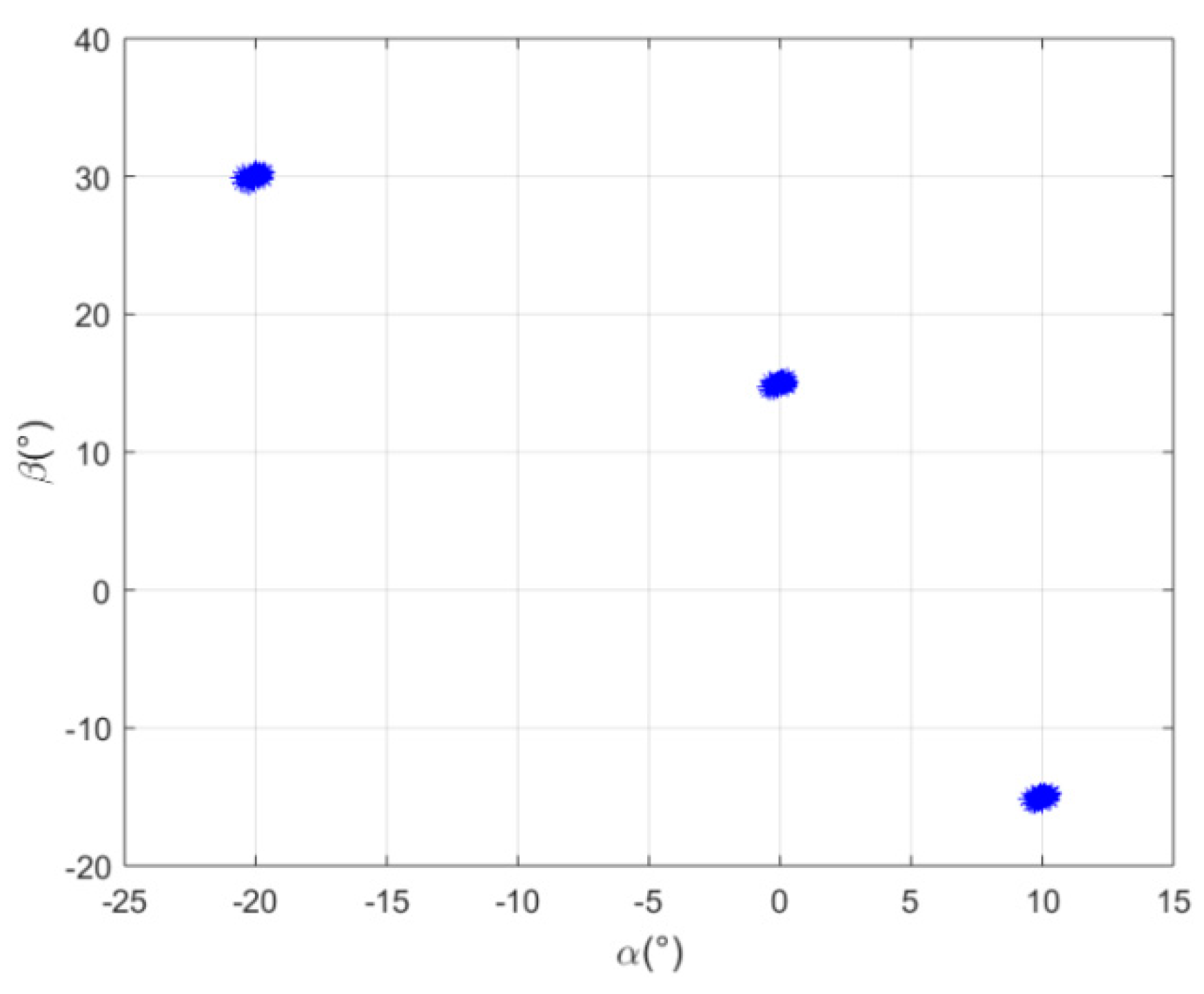
In the first simulation, the number of auxiliary array elements along x-axis and y-axis are set as N_x1 = 2 and N_y1 = 3, respectively, signal-to-noise ratio (SNR) is set as 10 dB, the Monte Carlo trial number is set as 50, and the number of snapshots is set as L = 256. Figure 2 shows the 2D DOAs estimated by the proposed algorithm.

Table 1. Mean and RMSE of the gain-phase error coefficients.

True Value	Estimated Gain Error Coefficients	RMSE of Gain Error Coefficients	Estimated Phase Error Coefficients (Rad)	RMSE of Phase Error Coefficients (Rad)
${\tilde{\Gamma }}_{00}=1.21\times e^{j0.12}$	1.2284	0.0229	0.1211	0.0130
${\tilde{\Gamma }}_{01}=1.1\times e^{j1.35}$	1.1344	0.0421	1.3530	0.0266
${\tilde{\Gamma }}_{02}=0.89\times e^{j0.98}$	0.9327	0.0524	0.9836	0.0403
${\tilde{\Gamma }}_{03}=1.35\times e^{j2.65}$	1.3825	0.0583	2.6551	0.0531
${\tilde{\Gamma }}_{10}=0.92\times e^{j1.97}$	0.9556	0.0925	1.9775	0.0681
${\tilde{\Gamma }}_{11}=0.94\times e^{j1.12}$	0.9594	0.0235	1.1221	0.0130
${\tilde{\Gamma }}_{12}=1.23\times e^{j2.35}$	1.2516	0.0615	2.3533	0.0245
${\tilde{\Gamma }}_{13}=1.49\times e^{j0.58}$	1.5154	0.0813	0.5848	0.0363

shows the mean and root mean square error (RMSE) of the gain-phase error coefficients obtained by the proposed algorithm, where only the first 8 gain-phase error coefficients of the original URA are given for simplification.

It can be seen from Figure 2 that the proposed algorithm can accurately estimate the 2D DOAs for the URA with gain-phase errors and the estimated 2D DOAs can be automatically paired. Therefore, it can achieve the localization of multiple sources. It can be seen from Table 1 that the proposed algorithm can also accurately estimate the gain-phase error coefficients, hence to further realize the self-calibration of the gain-phase errors of the URA.

5.2. 2D DOA Estimation Performance

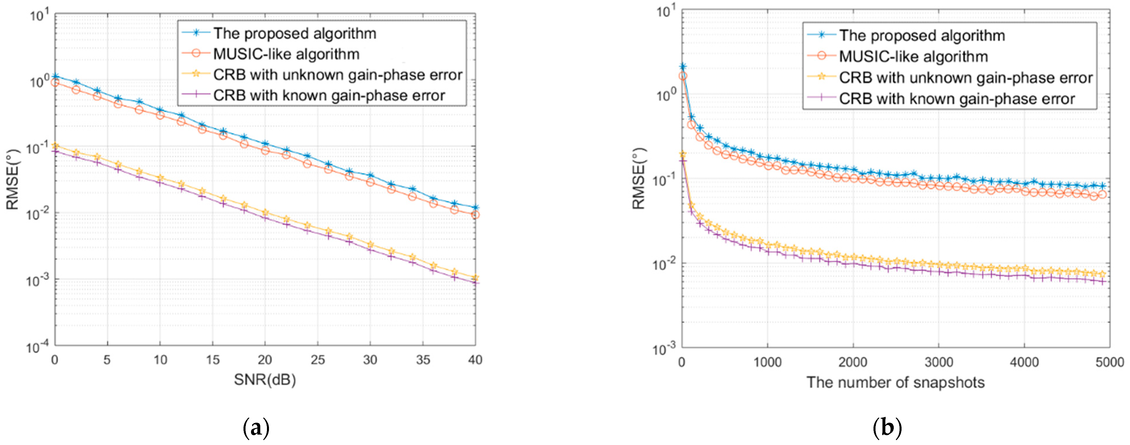
Using the same settings with Section 5.1, the proposed algorithm is assessed and compared with the MUSIC-like algorithm in [20] under different SNRs and different snapshots. Given L = 256, Figure 3a shows the 2D DOA estimation RMSEs of the proposed algorithm and the MUSIC-like algorithm with the SNR changing from 0 dB to 40 dB in a step of 2 dB. Given SNR = 10 dB, Figure 3b gives the 2D DOA estimation RMSEs of the proposed algorithm and the MUSIC-like algorithm with the snapshot number changing from 10 to 5000 in a step of 100. Both Figure 3a,b are obtained by averaging over 500 Monte Carlo trials. The theoretical CRB curves with unknown and known gain-phase error coefficients are also shown in Figure 3a,b.

It can be seen that, with the increase of the SNR and the snapshot number, the DOA estimation performance of both algorithms is gradually improved. Although its RMSEs are slightly larger than those of the MUSIC-like algorithm, the proposed algorithm can complete the 2D DOA estimation without any iteration and spectral peak search, hence has a much lower computing complexity (the running time of the proposed algorithm and the MUSIC-like algorithm are 0.2721 s and 1.9375 s, respectively).

5.3. Gain-Phase Error Self-Calibration Performance

Define the self-calibration errors of the gain error and phase error coefficients as $\Delta g={\Vert \widehat{g}-g\Vert }_2/{\Vert g\Vert }_2$ and $\Delta \mathit{\varphi }={\Vert \widehat{\mathit{\varphi }}-\mathit{\varphi }\Vert }_2/{\Vert \mathit{\varphi }\Vert }_2$, respectively, where $\widehat{g}$, $\widehat{\mathit{\varphi }}$ and $g$, $\mathit{\varphi }$ are the estimated and real error coefficients.

Given L = 256, Figure 4a,b show the self-calibration errors of the gain-phase error coefficients obtained by the proposed algorithm and the MUSIC-like algorithm with the SNR changing from 0 dB to 40 dB in a step of 2 dB. Given SNR = 10 dB, Figure 5a,b show the self-calibration errors of the gain-phase error coefficients obtained by the proposed algorithm and the MUSIC-like algorithm with the snapshot number changing from 10 to 5000 in a step of 100. The theoretical CRBs of the gain-phase error coefficient estimations are also shown in Figure 4 and Figure 5.

It can be seen from Figure 4 and Figure 5 that the self-calibration errors of the proposed algorithm are basically the same as that of the MUSIC-like algorithm in [20]. With the increase of the SNR and the snapshot number, the gain-phase self-calibration errors are progressively decreased, which means that the estimated gain-phase error matrix is close to the actual one, hence meeting the requirements of URA self-calibration.

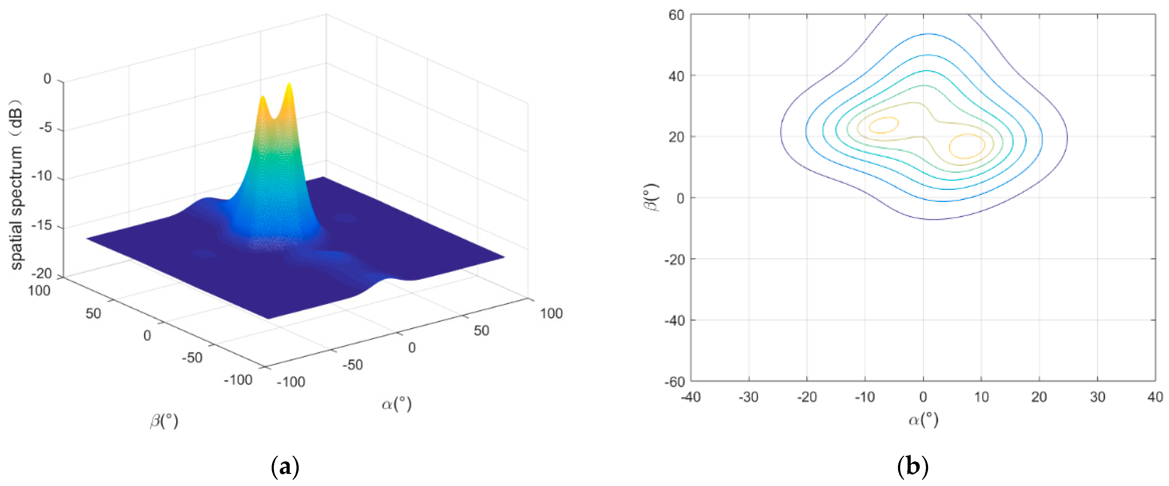
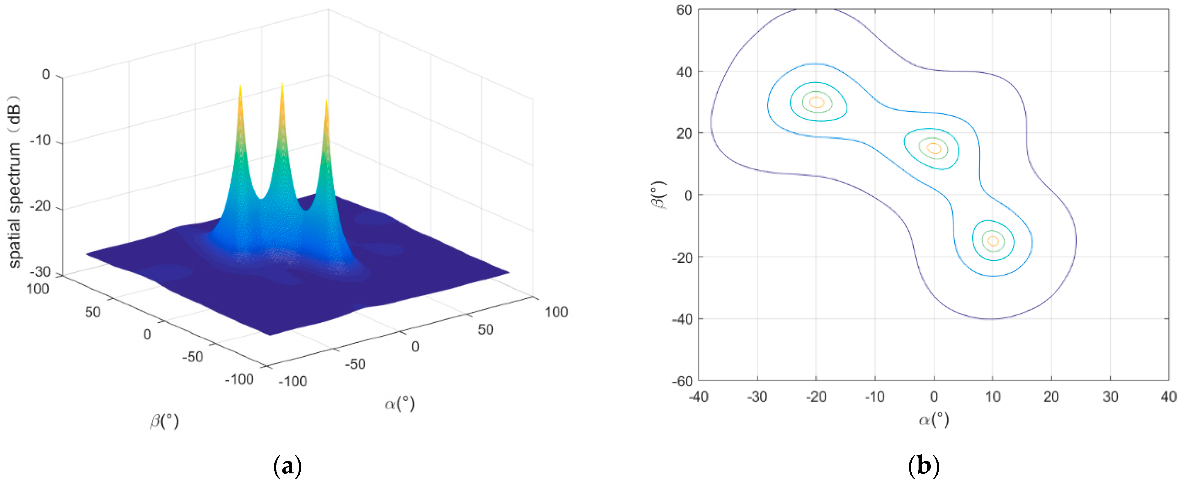
With and without gain-phase self-calibration by the proposed algorithm, Figure 6 and Figure 7 show the spatial spectra and the corresponding contour maps obtained by 2D MUSIC algorithm. In the simulation, the snapshots L = 256 and the SNR = 10 dB. It can be seen that, when the gain-phase error is not calibrated, the 2D MUSIC spatial spectrum cannot form accurate spectral peaks at the 2D DOAs of the three sources, thus the three sources cannot be distinguished. After gain-phase error self-calibration via the proposed algorithm, the 2D MUSIC spatial spectrum can form obvious and sharp spectral peaks at the 2D DOAs of the three sources. Therefore, the proposed algorithm can well accomplish the task of gain-phase error self-correction for the URA.

5.4. Performance Assessment under Different Numbers of Auxiliary Array Elements

The purpose of the final simulation is to assess the 2D DOA estimation performance of the proposed algorithm under different numbers of auxiliary array elements, so as to guide the application of the proposed algorithm in practice. Figure 8 shows the 2D DOA estimation RMSEs with the SNR changing from 0 dB to 40 dB in a step of 2 dB in the condition of $N_{x1}=2,$, $N_{y1}=2$, $N_{x1}=3,$, $N_{y1}=4$, and $N_{x1}=6,N_{y1}=5$ for different source numbers.

It can be seen that, with the increase of the number of auxiliary array elements, the 2D DOA estimation performance of the proposed algorithm will be slightly improved regardless of the source number and angular position, while the improvement is negligible compared to the cost of the additional auxiliary array elements. Hence, for practical URAs with gain-phase errors, the proposed algorithm only needs $N_{x1}=2$ and $N_{y1}=2$ auxiliary array elements for 2D DOA estimation.

6. Conclusions

Considering the gain-phase error of a URA, a low-complexity 2D DOA estimation and self-calibration algorithm is proposed in this study. First of all, the URA is modeled as the Kronecker product of two uniform linear arrays (ULAs), and several well-calibrated auxiliary elements are added into the two ULAs, respectively. Then, the rotation invariances destroyed by the gain-phase error are reconstructed by solving two constrained optimization problems, so that the ESPRIT algorithm can be used for 2D DOA estimation. Therefore, by setting several well-calibrated auxiliary array elements in the URA, the proposed algorithm can realize unambiguous joint 2D DOA and gain-phase error estimation. Simulation results indicate that the proposed algorithm can achieve high performance of 2D DOA estimation and gain-phase error self-calibration. Compared with existing typical algorithms, the proposed algorithm does not need any gain-phase error information during the DOA estimation process and does not need any iteration or peak search operations. Moreover, as the proposed algorithm does not need well-calibrated sources and does not use the small perturbation assumption of the array error, it is more suitable for the actual applications.

References

1. Abeida, H.; Delmas, J.P. Robustness of subspace-based algorithms with respect to the distribution of the noise: Application to DOA estimation. Signal Process. 2019, 164, 313–319. [Google Scholar] [CrossRef] [Green Version]
2. Zhang, S.M.; Ahmed, A.; Zhang, Y.D.; Sun, S.Q. Enhanced DOA estimation exploiting multi-frequency sparse array. IEEE Trans. Signal Process. 2021, 69, 5935–5946. [Google Scholar] [CrossRef]
3. Luo, J.; Zhang, Y.; Yang, J.; Zhang, D.; Zhang, Y.; Zhang, Y.; Huang, Y.; Jakobsson, A. Online sparse DOA estimation based on sub–aperture recursive LASSO for TDM–MIMO radar. Remote Sens. 2022, 14, 2133. [Google Scholar] [CrossRef]
4. Fu, X.W.; Cao, R.Z.; Wen, F.Q. A de-noising 2D-DOA estimation method for uniform rectangle array. IEEE Commun. Lett. 2018, 22, 1854–1857. [Google Scholar] [CrossRef]
5. Yu, J.; Li, J.; Sun, B.; Jiang, Y.; Xu, L. Multiple RFI sources location method combining two-dimensional ESPRIT DOA estimation and particle swarm optimization for spaceborne SAR. Remote Sens. 2021, 13, 1207. [Google Scholar] [CrossRef]
6. Li, J.; Zhao, J.; Ding, Y.H.; Li, Y.F.; Chen, F.J. An improved co-prime parallel array with conjugate augmentation for 2-D DOA estimation. IEEE Sens. J. 2021, 21, 23400–23411. [Google Scholar] [CrossRef]
7. Chen, P.; Chen, Z.M.; Cao, Z.X.; Wang, X.B. A new atomic norm for DOA estimation with gain-phase errors. IEEE Trans. Signal Process. 2020, 68, 4293–4306. [Google Scholar] [CrossRef]
8. Wan, B.; Wu, X.; Yue, X.; Zhang, L.; Wang, L. Calibration of phased-array high-frequency radar on an anchored floating platform. Remote Sens. 2022, 14, 2174. [Google Scholar] [CrossRef]
9. See, C.M.S. Method for array calibration in high-resolution sensor array processing. IEE Radar Sonar Navig. 1995, 142, 90–96. [Google Scholar] [CrossRef]
10. Astely, D.; Swindlehurst, A.L.; Ottersten, B. Spatial signature estimation for uniform linear arrays with unknown receiver gains and phases. IEEE Trans. Signal Process. 1999, 47, 2128–2138. [Google Scholar] [CrossRef] [Green Version]
11. Kim, J.; Yang, H.J.; Jung, B.W.; Chun, J. Blind calibration for a linear array with gain and phase error using independent component analysis. IEEE Antennas Wirel. Propag. Lett. 2010, 9, 1259–1262. [Google Scholar] [CrossRef]
12. Liao, B.; Chan, S.C. Direction-of-arrival estimation in subarrays-based linear sparse arrays with gain/phase uncertainties. IEEE Trans. Aerosp. Electron. Syst. 2013, 49, 2268–2280. [Google Scholar] [CrossRef]
13. Xie, W.; Wang, C.S.; Wen, F.; Liu, J.B.; Wan, Q. DOA and gain-phase errors estimation for noncircular sources with central symmetric array. IEEE Sens. J. 2017, 17, 3068–3078. [Google Scholar] [CrossRef]
14. Tian, Y.; Wang, Y.R.; Rong, X.R.; Lian, Q.S. Mixed source localization and gain-phase perturbation calibration in partly calibrated symmetric uniform linear arrays. Signal Process. 2020, 166, 1–7. [Google Scholar] [CrossRef]
15. Hu, B.; Wu, X.C.; Zhang, X.; Yang, Q.; Deng, W.B. DOA estimation based on compressed sensing with gain/phase uncertainties. IET Radar Sonar Navig. 2018, 12, 1346–1352. [Google Scholar] [CrossRef]
16. Fang, Y.F.; Zhu, S.Q.; Gao, Y.C. Direction finding by covariance matrix sparse representation with sensor gain and phase uncertainties in unknown non-uniform noise. IEEE Wirel. Commun. Lett. 2021, 10, 175–179. [Google Scholar] [CrossRef]
17. Liu, A.F.; Liao, G.S.; Zeng, C.; Yang, Z.W.; Xu, Q. An eigenstructure method for estimating DOA and sensor gain-phase errors. IEEE Trans. Signal Process. 2011, 59, 5944–5956. [Google Scholar] [CrossRef]
18. Philipp, H.; Abdelhak, M.Z.; Michael, R. Joint 2-D DOA estimation and phase calibration for uniform rectangular arrays. IEEE Trans. Signal Process. 2012, 60, 4683–4693. [Google Scholar]
19. Yuan, L.T.; Jiang, R.X.; Chen, Y.W. Gain and phase autocalibration of large uniform rectangular arrays for underwater 3-D sonar imaging systems. IEEE J. Ocean. Eng. 2014, 39, 458–471. [Google Scholar] [CrossRef]
20. Cui, H.; Peng, W.J.; Liu, T. MUSIC-like joint estimation of 2-D DOAs and sensor gain/phase responses for rectangular array. In Proceedings of the 2017 11th Asian Control Conference (ASCC), Gold Coast, QLD, Australia, 17–20 December 2017. [Google Scholar]
21. Dai, Z.; Su, W.M.; Gu, H. A gain and phase autocalibration approach for large-scale planar antenna arrays. IEEE Commun. Lett. 2021, 25, 1645–1649. [Google Scholar] [CrossRef]
22. Wang, B.H.; Wang, Y.L.; Chen, H.; Guo, Y. Array calibration of angularly dependent gain and phase uncertainties with carry-on instrumental sensors. Sci. China Ser. F Inf. Sci. 2004, 47, 777–792. [Google Scholar] [CrossRef]
23. Mao, Z.; Liu, S.; Qin, S.; Haung, Y. Cramér-Rao Bound of joint DOA-range estimation for coprime frequency diverse arrays. Remote Sens. 2022, 14, 583. [Google Scholar] [CrossRef]
Figure 1. Geometry of the original and extended URAs for 2D DOA estimation.
Remotesensing 14 03064 g001
Figure 2. The estimated 2D DOAs.
Remotesensing 14 03064 g002
Figure 3. The RMSEs of 2D DOA estimation. (a) RMSE versus SNR; (b) RMSE versus snapshots.
Remotesensing 14 03064 g003
Figure 4. The self-calibration errors versus SNR. (a) Δ g versus SNR; (b) Δ ϕ versus SNR.
Remotesensing 14 03064 g004
Figure 5. The self-calibration errors versus snapshot number. (a) Δ g versus snapshot number; (b) Δ ϕ versus snapshot number.
Remotesensing 14 03064 g005
Figure 6. 2D MUSIC estimation results without self-calibration. (a) Spatial spectrum; (b) Contour map.
Remotesensing 14 03064 g006
Figure 7. 2D MUSIC estimation results with self-calibration. (a) Spatial spectrum; (b) Contour map.
Remotesensing 14 03064 g007
Figure 8. DOA estimation RMSE with different auxiliary array elements for different source numbers. (a) 1 source located on ( 25 , 30 ) ; (b) 3 sources located on ( 20 , 30 ) , ( 0 , 15 ) , and ( 10 , 15 ) .
Remotesensing 14 03064 g008