
Detection of River Plastic Using UAV Sensor Data and Deep Learning
by
 , , ,
, , ,
Nisha Maharjan
1,* ,
,
Hiroyuki Miyazaki
1,2 ,
,
Bipun Man Pati
3,
Matthew N. Dailey
1,
Sangam Shrestha
4 and
Tai Nakamura
1 1
Department of Information and Communication Technologies, School of Engineering and Technology, Asian Institute of Technology, Pathum Thani 12120, Thailand
2
Center for Spatial Information Science, The University of Tokyo, Chiba 277-8568, Japan
3
Faculty of Pharmaceutical Sciences, Chulalongkorn University, 254 Phayathai Road, Patumwan District, Bangkok 10330, Thailand
4
Department of Civil and Infrastructure Engineering, School of Engineering and Technology, Asian Institute of Technology, Pathum Thani 12120, Thailand
*
Author to whom correspondence should be addressed.
Remote Sens. 2022, 14(13), 3049; https://doi.org/10.3390/rs14133049
Submission received: 9 May 2022
/
Revised: 19 June 2022
/
Accepted: 22 June 2022
/
Published: 25 June 2022
(This article belongs to the Special Issue Deep Learning and Computer Vision in Remote Sensing)
Abstract
:Plastic pollution is a critical global issue. Increases in plastic consumption have triggered increased production, which in turn has led to increased plastic disposal. In situ observation of plastic litter is tedious and cumbersome, especially in rural areas and around transboundary rivers. We therefore propose automatic mapping of plastic in rivers using unmanned aerial vehicles (UAVs) and deep learning (DL) models that require modest compute resources. We evaluate the method at two different sites: the Houay Mak Hiao River, a tributary of the Mekong River in Vientiane, Laos, and Khlong Nueng canal in Talad Thai, Khlong Luang, Pathum Thani, Thailand. Detection models in the You Only Look Once (YOLO) family are evaluated in terms of runtime resources and mean average Precision (mAP) at an Intersection over Union (IoU) threshold of 0.5. YOLOv5s is found to be the most effective model, with low computational cost and a very high mAP of 0.81 without transfer learning for the Houay Mak Hiao dataset. The performance of all models is improved by transfer learning from Talad Thai to Houay Mak Hiao. Pre-trained YOLOv4 with transfer learning obtains the overall highest accuracy, with a 3.0% increase in mAP to 0.83, compared to the marginal increase of 2% in mAP for pre-trained YOLOv5s. YOLOv3, when trained from scratch, shows the greatest benefit from transfer learning, with an increase in mAP from 0.59 to 0.81 after transfer learning from Talad Thai to Houay Mak Hiao. The pre-trained YOLOv5s model using the Houay Mak Hiao dataset is found to provide the best tradeoff between accuracy and computational complexity, requiring model resources yet providing reliable plastic detection with or without transfer learning. Various stakeholders in the effort to monitor and reduce plastic waste in our waterways can utilize the resulting deep learning approach irrespective of location.
1. Introduction
Plastic is used extensively in households and industry. Plastic takes hundreds of years to degrade, so it affects both the terrestrial and marine ecosystems. Marine litter has been recognized as a serious global environmental issue since the rise of the plastic industry in the mid-1950s [1]. Hence, the need for research into plastic management solutions is self-evident [2]. The UN Environment Programme (UNEP) estimates that 15% of marine litter floats on the sea’s surface, 15% remains in the water column, and 70% rests on the seabed. Up to 80% of the plastic in the ocean is from land-based sources and reaches the ocean via rivers [3]. Nevertheless, riverine plastics are understudied compared to marine plastics [4]. The earliest research on riverine plastic began in the 2010s, with a study on a sample of waterways in Europe and North America, particularly the Los Angeles area [5] and the Seine [6].
Current government regulations do not adequately address marine litter and plastics. There is also a gap in regional frameworks addressing the issue of plastic litter. Establishing proper waste collection systems and changing peoples’ perceptions are two major hurdles to plastic litter prevention, and both goals remain a distant dream in southeast Asian countries. Thoroughly surveying plastic litter distribution in rural areas manually is time-consuming and complex, so automatic mapping of plastic litter using unmanned aerial vehicles (UAVs) is a better option, especially in inaccessible locations.
UAVs (abbreviations used throughout the paper are listed in “Abbreviations” in alphabetical order) are relatively low-cost and can operate at low-altitudes with minimal risk. They provide images with high resolution and high image acquisition frequency [7]. UAV-based real-time data collection of imagery is important for surveillance, mapping, and disaster monitoring [8,9]. UAVs are widely used for data collection, object detection, and tracking [10]. UAVs can be categorized as low- or high-altitude platforms [11] and can be roughly categorized into three classes: small, medium, and large, according to their maximum altitude and range. The maximum altitude for small drones is usually below 300 m; the maximum altitude for large drones is normally above 5500 m. Altitudes vary within these ranges for medium size UAVs. Regarding maximum range, small UAVs can typically cover less than 3 km, while medium UAVs can cover 150–250 km, and large ones can cover even larger distances. High-altitude UAVs can image large areas quickly, while low attitude UAVs can capture more detailed features in smaller fields of view. High-altitude UAV scans can be used as a preliminary to reduce the overhead involved in finding the correct areas for more detailed surveys. Once a high-altitude survey is completed, the plastic in a river can be precisely detected and catalogued based on a follow-up low-altitude UAV survey. Since UAVs at such low-altitudes can provide centimeter-level or better pixel resolution with high accuracy [12], they open the door for ordinary individuals to collect and analyze high-quality imagery through automatic methods irrespective of whether satellite or aerial imagery is available from formal sources. Given a specific camera selected and mounted on a UAV, an appropriate flight altitude should be determined to obtain a suitable ground sampling distance (GSD) for measuring sizes of items captured in the images and for efficiently covering the target area. The GSD is the size of the projection of one pixel on the ground and is a function of the focal length of the camera, flight altitude, and physical dimensions of sensor’s pixels. The GSD places a lower limit on the precision achievable for points on the ground [13]. In addition, flight altitude, camera properties determine the resolution of the images captured. Though we obtain good resolution with a 4K camera at 30 m, other researchers [13,14,15] conducted flights at ranges of 6–10 m for better image resolution. UAVs flying at a low-altitude provide high-resolution data, which are useful in detecting plastic, metal, and other litter in rivers. The focal length also affects image quality and plays a vital role in obtaining accurate annotations and precise plastic detection [16]. Simple color-based approaches to categorization of litter in UAV images [17] are less dependent on flight altitude and GSD than object detectors, which typically require high resolution images captured at lower altitudes.
UAVs have already been used in monitoring marine macro-litter (2.5 cm to 50 cm) in remote islands [18,19,20], which suggests that low-cost UAVs are suitable for low-altitude, high-resolution surveys (from 6 m to 30 m). Estimates of plastic litter in global surface waters are available [2], but we are far from having a global inventory of litter along shores due to the low efficiency and limited extent of surveys along shores thus far [21]. However, UAV images have been found effective for analyzing the spatial distribution of plastic litter cross-shore and long-shore, as well as for measuring the sizes of detected items using semi-automated image processing techniques [22]. Moreover, UAV applications were found to be effective for monitoring coastal morphology, the extent of morphological changes, and interaction of marine litter dynamics on the beach [23].
Floating litter surveys conducted by UAVs at altitudes of 20 m and 120 m have been found to be more accurate than beach litter surveys at altitudes of 20 m and 40 m [24]. The authors attribute this to seawater being a more homogeneous background than sand. Floating litter surveys, however, have the risk of losing the UAV while it is flying over the sea, and beach litter surveys are less affected by environmental challenges. According to Martin et al. [20], manual screening of UAV images of beaches taken from a height of ten meters was 39 times faster and 62% more accurate than the standard ground-based visual census method. Researchers also pointed out that training citizen scientists to annotate plastic litter datasets acquired through UAVs is effective [25,26]. However, machine learning-based automatic mapping combined with manual screening was found to be even faster and more cost-effective [19,20].
Since rigorous interpretation of aerial images from UAVs by humans is time-consuming, error-prone, and costly, modern deep learning (DL) methods using convolutional neural networks (CNNs) are a preferable alternative [27]. DL is already well established in remote sensing analysis of satellite images. UAV technology integrated with deep learning techniques is now widely used for disaster monitoring in real time, yielding post-disaster identification of changes with very higher accuracy [28,29]. DL has emerged as an extremely effective technique in modern computer vision due to its ability to handle a variety of conditions, such as scale transformations, changes in background, occlusion, clutter, and low resolution, partly due to model capacity and partly due to the use of extensive image augmentation during training [30]. DL has proven superior to traditional machine learning techniques in many fields of computer vision, especially object detection, which involves precise localization and identification of objects in an image [17,31]. Classification, segmentation, and object detection in multispectral ortho imagery through CNNs has been successful [32]. In UAV mapping applications involving detection of objects, changes in viewing angles and illumination introduce complications, but CNNs nevertheless extract useful distinguishable features. CNNs are very effective for per-pixel image classification.
Although deep learning methods have been shown to provide accurate and fast detection of marine litter [33], little research integrating UAVs and deep learning has been conducted in the context of monitoring plastics on beaches and rivers. Once a model has been trained, processing UAV images for detection of plastics with the model is straightforward. However, deep learning methods require a great deal of computing resources for offline training and online inference, as models are required to perform well across various conditions, increasing their complexity. Furthermore, training of modern object detection models requires a great deal of manual labor to label data, as the data preparation requires accurate bounding boxes in addition to class labels, making the data engineering more intensive than that required for classification models. To minimize these costs, plastic monitoring application should analyze georeferenced UAV patch images ensuring appropriate image quality and little redundancy. To determine whether a given training dataset is sufficiently representative for the plastic detection in similar georeferenced patch images after model development, we advocate evaluation of the method at multiple locations.
It is time consuming to train a deep neural network for detection from scratch. It can be more effective to fine-tune an existing pre-trained model on a new task without defining and training a new network, gathering millions of images, or having an especially powerful GPU. Using a pre-trained network as a beginning point rather than starting from scratch (called transfer learning) can help accelerate learning of features in new datasets with small amounts of training data while avoiding overfitting. This approach is therefore potentially particularly useful for detection of plastic in a modest-scale dataset. OverFeat [34], the winner of the localization task in the ILSVRC2013 competition, used transfer learning. Google DeepMind uses transfer learning to build deep Q-network agents that use pixels from 210 × 160 color video at 60 Hz and the game score as input and learn new games across different environments with the same algorithms and minimal knowledge. This model was the first artificial agent to learn a wide variety of challenging tasks without task-specific engineering [35]. Nearly every object detection method in use today makes use of transfer learning from the ImageNet and COCO datasets. The use of transfer learning provides the following advantages [36]:
- higher baseline performance;
- less time to develop the model;
- better final performance.
We therefore investigated the performance of pretrained and tabula rasa object detection models for plastic detection using data acquired from a Mekong river tributary, the Houay Mak Hiao (HMH) river in Vientiane, Laos, as well as a canal in the Bangkok area, Khlong Nueng in Talad Thai (TT), Khlong Luang, Pathum Thani, Thailand. We explored how a model trained on one location performs in a different location in terms of compute resources, accuracy, and time.
This paper makes three main contributions to the state of the art in riverine plastic monitoring:
- We examine the performance of object detection models in the You Only Look Once (YOLO) family for plastic detection in ortho imagery acquired by low-altitude UAVs.
- We examine the transferability of the knowledge encapsulated in a detection model from one location to another.
- We contribute a new dataset comprising images with annotations for the public to use to develop and evaluate riverine plastic monitoring systems.
We believe that this research will provide practitioners with tools to save computing resources and manual labor costs in the process of developing deep learning models for plastic detection in rivers. The techniques introduced here should scale up to various types of landscapes all over the world.
2. Materials and Methods
In this section, we describe the study area for the research and the materials and methods adopted to perform experiments on the task of plastic detection from UAV imagery in two locations through deep learning.
2.1. Study Area
We gathered data at two locations, viz., Khlong Nueng Canal, Talad Thai, Pathum Thani (TT), Thailand and Houay Mak Hiao river in Vientiane, Laos (HMH) as in Figure 1. HMH is in a sub-basin of the Mekong River basin with a land area of 436.91 km2, located in Vientiane, the capital city of Laos as in Figure 2. The study area was at coordinates 17.95°N 102.91°E. This river contributes pollutant to the Mekong River basin. TT is in Khlong Luang district, Thailand with coordinates 14.08°N 100.62°E, as shown in Figure 3. The study areas were selected based on their contribution to pollution downstream and the ease and safety of accessibility for data collection considering UAV survey zone restriction in Laos and Thailand. As no study of individual plastic object detection in these areas has yet been performed, they were found to be ideal for evaluating plastic monitoring methods.
2.2. Materials
UAV surveys 30 m above the terrain were carried out at Houay Mak Hiao river (HMH) in Vientiane, Laos and Khlong Nueng Canal (TT) in Talad Thai, Pathum Thani, Thailand with a DJI Phantom 4 with a 4K resolution camera resulting in a ground sampling distance of 0.82 cm to assess the plastic monitoring methods for these waterways.
The computing resources comprised two environments: (1) Anaconda with Jupyter running on a personal computer with an Intel®Core™ i7-10750H CPU @2.60 GHz, 16 GB RAM, and NVIDIA GeForce RTX 2060 GPU with 6 GB GPU RAM, and (2) Google Colaboratory Pro. The personal computer was used for YOLOv3 and YOLOv5, and Google Colaboratory Pro was used for YOLOv2 and YOLOv4.
2.3. Methodology
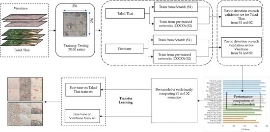
In this section, the proposed methodology for detection of plastic in rivers is discussed, along with the various deep learning model architectures used in the experiments. We aim to assess model performance in the task of identifying plastic in rivers using georeferenced ortho-imagery and deep learning approaches utilizing minimal computing resources, as shown in Figure 4.
2.3.1. Deep Learning Models for Object Detection
CNNs can locate multiple objects in an image, effectively separating foreground from background [37]. We thus evaluate various CNN-based object detection models on riverine plastic detection. Object detection has two main functions: to find regions of interest and to classify those regions. Regions of interest can be obtained in two ways, by region proposal methods or direct regression. Region proposal methods involve two stages, the first of which involves finding regions of interest through color contrast and superpixel straddling, and the second of which involves classifying the resulting proposals with CNNs. The direct regression method, on the other hand, is a one step-method in which region proposals and object detection are carried out in a single step. Single-step models tend to find it difficult to locate small objects in an image due to a limited number of possible bounding boxes at fine levels of detail. YOLO is the most popular single-stage detector. It carries out both the bounding box identification and object classification tasks in a single pass of the network. R-CNN is a representative of two-stage detectors. Some of the older detection models use a full CNN classifier such as VGG-16 or ResNet as the classifier while most modern detectors such as YOLO use a CNN classifier as a backbone for feature extraction followed by a small “head” for classification.
Early versions of YOLO had better performance in both speed and accuracy than extant models such as MobileNetSSDv2 and Faster R-CNN. YOLO makes use of a single CNN to detect objects by processing the entire image at once without creating region proposals. It predicts a detection tensor directly based on a small set of possible bounding boxes. Features at the deeper layers used for the final detection have receptive fields spanning the entire image, making it less likely to predict false positives in background regions. YOLO models output bounding box coordinates, confidence scores, and object class scores directly with an image as input. The confidence scores signify the probability that a predicted box contains an object. YOLO is fast, running at 45 FPS in real-time, and Fast YOLO is faster at 155 FPS [38]. The original YOLO architecture predicts just two bounding boxes per grid cell [39]. The total of 98 bounding boxes per image is small compared to the 2000 boxes predicted by Selective Search. Though most of the early detection frameworks depended on heavy feature extractors such as VGG-16, which uses 30.69 billion floating operations in a single pass for a single image of 224 × 224 resolution, YOLO used the more lightweight GoogLeNet architecture, with only 8.52 billion operations [40], albeit with lower accuracy as a backbone than VGG-16. YOLO has no localization error and hence is less likely to predict false positives in the background [41].
YOLOv2 was introduced to improve the speed-accuracy trade-offs in YOLO. The custom GoogLeNet [42] network was replaced by DarkNet19, and batch normalization [43] was introduced. The fully connected layers in GoogLeNet were also removed, and anchor boxes with aspect ratios learned through k-means were introduced along with multiscale training. Despite these improvements, YOLOv2 has low recall [38], so YOLOv3 was subsequently introduced with further improvements. YOLOv3 is tuned for small objects with multi-scale features [44]. YOLOv3 is much more complicated than the previous model, and the speed and accuracy can be varied by changing model size. YOLOv3 provides good average precision (AP) at an Intersection over Union (IoU) threshold of 0.5, but the AP decreases at higher IoU levels because YOLOv3 does not predict ground truth bounding box boundaries very accurately. YOLOv3-SPP (spatial pyramid pooling) adds a SPP module, which uses the concept of the spatial feature pyramid, realizing both local and global features. This solves the issue of image distortion caused by cropping and zooming the image area and repeated feature extraction by the CNN. The smaller version of YOLOv3, called Tiny YOLOv3, is designed for mobile machine learning and low-powered computing devices such as the Internet of Things (IoT) devices and shows better performance in terms of speed accordingly [45]. The size of the Tiny YOLOv3 CNN is about 20% that of YOLOv3, and it runs several times faster, making it usable for real-time detection on small devices. From YOLOv2 to YOLOv3, the computational complexity in terms of GFLOPs (billion floating-point operations), which mostly depends on the number and types of layers used in the network, increases from 30 to 140, with an increase in mAP from 21% to 33%. The added complexity, however, means it cannot be considered a light-weight model [44].
YOLOv4 and YOLOv5 were developed to increase the speed of YOLOv3 while keeping high accuracy. YOLOv3 was known not to perform well on images with multiple features or on small objects. Among other improvements, YOLOv4 uses the Darknet53 backbone augmented with cross-stage partial blocks (CSPDarknet53), improving over YOLOv3 using only 66% of the parameters of YOLOv3, accounting for its fast speed and accuracy [46]. The YOLOv5 model pushes this further, with a size of only 27 megabytes (MB), compared to the 244 MB of YOLOv4. YOLOv5 models pre-trained on MS COCO achieve mAPs from 36.8% (YOLOv5s) to 50.1% (YOLOv5x). YOLOv5 and YOLOv4 have similar network architectures; both use CSPDarknet53 as the backbone, and both use a path aggregation network (PANet) and SPP in the neck and YOLOv3 head layers. YOLOv5’s reference implementation is based on the PyTorch framework for training rather than the Darknet C++ library of YOLOv4. This makes YOLOv5 more convenient to train on a custom dataset to build a real time object detection model.
Yao et al. [47] consider the fact that UAVs normally capture images of objects with high interclass similarity and intraclass diversity. Under these conditions, anchor-free detectors using point features are simple and fast but have unsatisfactory performance due to losing semantic information about objects resulting from their arbitrary orientations. The authors’ solution uses a stacked rotation convolution module and a class-specific semantic enhancement module to extract points with representations that are more class-specific, increasing mAP by 2.4%. Future work could compare YOLO-type detectors with improved point feature-based detectors such as R2 IPoints. However, it is difficult to detect small objects with dense arrangements using this detector due to the sensitiveness of IoU to the deviation of the position of small objects.
The use of transformer neural networks [48] has led a new direction in computer vision. Transformers use stacked self-attention layers to handle sequence-to-sequence tasks without recursion, and transformers have recently been applied to vision tasks such as object detection. The vision Transformer (ViT) was the first high accuracy transformer for image classification [49]. However, ViT can only use small-sized images as input, which results in loss of information. The detection transformer (DETR) [50] performs object detection and segmentation. DETR matches the performance of highly optimized Faster R-CNN on the COCO dataset [51]. The Swin transformer [52] has been proposed as a backbone for computer vision. Swin stands for shifted window which is a general-purpose backbone for computer vision. Swin is a hierarchical transformer that limits the self-attention computation to non-overlapping local windows and allows cross-window connection through shifted window to address the issue of a large variation in scale and resolution of images, leading to relatively good efficiency on general hardware, running in time linear in the image size. The Swin transformer achieves current state-of-the-art performance on the COCO object detection task (58.7 box AP and 51.1 mask AP on COCO test-dev) and ADE20K semantic segmentation (53.5 mIoU on ADE20Kval).
CNNs have a natural inductive bias for image processing problems, such as translation equivariance and contrast adaptivity, but the transformer lacks these properties, resulting in requirements for much larger datasets or stronger data enhancement [53] to achieve the best performance. Since our goal is to perform well on moderate-sized datasets using modest compute resources, we do not consider transformers at this time.
2.3.2. Selection of Object Detection Models
Various object detection models have been used in research related to plastic litter detection. Majchrowska et al. [54] use EfficientDet-D2 to localize litter and EfficientNet-B2 to classify waste into seven categories. The researchers obtained 75% classification accuracy and 70% mean average precision.
Córdova et al. [55] conducted a comparative study on state-of-the-art approaches for object detection using the PlastOPol and TACO datasets and found that YOLOv5-based detectors perform well in litter detection. On the PlastOPol dataset, YOLO-v5x obtains a best [email protected] of 84.9, and YOLO-v5s obtains best [email protected] of 79.9. On the TACO dataset, YOLO-v5x obtains a best [email protected] of 63.3, and YOLO-v5s obtains a best [email protected] of 54.7 for YOLO-v5s. YOLO-v5s was found to be 4.87, 5.31, 6.05, and 13.38 times faster than RetinaNet, Faster R-CNN, Mask R-CNN, and EfficientDet-d5, respectively.
Kraft et al. [56] use calibrated onboard cameras with GNSS and GPS to capture images and use YOLOv3, YOLOv4, and EfficientDet for object detection [57]. They find that YOLOv4 and EfficientDet-d3 show the highest mean average precision (mAP) for trash detection. Kumar et al. [58] analyze the efficiency of YOLOv3 and YOLOv3-tiny in separating waste into bio-degradable and non-biodegradable types. Their research shows that YOLOv3 has better predictive performance than YOLOv3-tiny, with accuracies of 85.29% and 26.47%, respectively. This research used 6437 images drawn from six classes (cardboard, paper, glass, plastic, metal, and organic waste) and found that YOLOv3-tiny needs four times less computation time than YOLOv3, demonstrating a wide speed-accuracy tradeoff.
Fulton et al. [59] evaluate the performance of object detection algorithms (YOLOv2, Tiny-YOLO, Faster R-CNN with Inception v2, and Single Shot MultiBox Detector (SSD) with MobileNetV2 for underwater trash detection and removal of trash using autonomous underwater vehicles. (AUVs). The models detect three classes of objects in the J-EDI (JAMSTEC E-Library of Deep-Sea Images) dataset, i.e., plastic, remotely operated vehicles (ROVs), and a “bio” class (plants, fish, detritus, etc.). All the above-mentioned models are fine-tuned from their pre-trained states. The authors’ transfer learning method for the YOLO model only updates weights in the last three layers. The authors find that the YOLOv2 models have good speed, but YOLOv2 and tiny-YOLO have low mAP. They also find that transfer learning increases accuracy for the bio-class to a level sufficient for deployment in real time scenarios.
Tata et al. [60] describe the DeepPlastic project for marine debris detection in the epipelagic layer of the ocean. This project includes the development of the DeepTrash dataset comprising annotated data captured from videos of marine plastic using off-the-shelf cameras (GoPro Hero 9) in three study sites in California (South Lake Tahoe, Bodega Bay, and San Francisco Bay) and also incorporating the J-EDI dataset to represent marine plastics in different locations. The research used low-cost GPUs and the deep learning architectures YOLOv4-tiny, Faster R-CNN, SSD, and YOLOv5s for detection with the aim to build a real-time monitoring system. The YOLOv5s model achieved a mAP of 85%, which is higher than that of the YOLOv4-tiny model (84%). These models outperformed a model for detection of deep-sea and riverine plastic by the University of Minnesota [59], which had mAPs of 82.3% using YOLOv2 and 83.3% using Faster R-CNN. The authors therefore selected YOLOv4-tiny and YOLOv5s, which have good accuracy and sufficiently high inference speeds for real-time object detection. Since there are several models with different speed-accuracy tradeoffs in the YOLOv5 group of detectors, various YOLOv5 models have been used in research related to the detection of plastic [61]. This family of object detection models offers flexibility in terms of architecture and can be adjusted for the best performance in different tasks. From YOLOv5s to YOLOv5l, the number of parameters, depth, and width increases steadily resulting in higher model complexity but better accuracy. We use the YOLO family of algorithms for plastic detection in the river in this research due to its good performance in terms of speed and accuracy of detection in real-world environments with limited computing resources and data. We trained different pre-trained YOLOv2 models (YOLOv2, YOLOv2-tiny), YOLOv3 models (YOLOv3, YOLOv3-tiny, and YOLOv3-spp), YOLOv4 models (YOLOv4, YOLOv4-tiny), and YOLOv5 models (YOLOv5s, YOLOv5m, YOLOv5l, YOLOv5x) to perform plastic detection in UAV images. In addition, fine-tuning the pre-trained models, we also trained each of the aforementioned models from scratch to determine which approach performs best with limited time and capacity. As previously discussed, YOLOv5s was previously found to perform best for plastic detection in the epipelagic layer of the ocean, with a mAP of 0.851 [60], so we use a similar methodology to evaluate performance of plastic detection models for rivers using various YOLO architectures according to mAP at different IoUs.
2.3.3. Transfer Learning
Training deep CNNs from scratch is difficult, as they need a large amount of training data and labeling expertise. Transfer learning can speed up model development compared to training from scratch by fine-tuning some or all of the layers of a pretrained network to perform well on a new dataset [62]. Transfer learning reduces training time, as the model does not need to be trained for many iterations to give good performance. There are two methods of transfer learning, feature extraction and fine-tuning. Feature extraction uses knowledge of features learned on one model to extract meaningful features from a new dataset. In this transfer learning setup, weights of the feature extraction portion of the pre-trained network are not updated during training on the new dataset. Instead, some of the deepest layers are unfrozen, and the model is trained with a low learning rate for both the new classifier layer and the previously existing deepest layers of the base model. Transfer learning via fine-tuning, on the other hand, allows all the layers or some of the layers of the base model to be unfrozen, and model is retrained end-to-end, again with a very low learning rate. The outcome is to fine-tune the weights of the pre-trained network to extract high-order features more appropriate for the specific new task.
2.3.4. Performance Assessment of Transfer Learning
In addition, in-sample test performance, we also assess each model’s capacity for knowledge transfer to another location. Deep learning models learn features representative of their training datasets. Early layers tend to learn general features, while later layers tend to learn features that are high level and more specific to the training dataset. We perform transfer learning on models pre-trained on one location, fine-tuning them by either (1) freezing weights of all the initial layers of the network of the pre-trained models and then changing the weights of the last two layers of the respective network, allowing them to learn features from data of the new location, or (2) fine-tuning all parameters in every layer. The best weights for the best model for plastic detection at one location are used as a basis for training at the other location. The same performance metrics are computed for each of the transferred models to find the best approach to transfer learning about the plastic detection task to a new location at low computing cost with minimal compute time.
The following basic steps are required to perform the comparison of deep learning techniques.
- Data preparation: Prepare the data set in the appropriate format (e.g., DarkNet format for YOLOv4-tiny and PyTorch format for YOLOv5s) and then split it into training and validation sets.
- Input: Prepare images and label files for training and validation dataset along with the pre-trained weights and configuration file for training.
- Output: Save trained model to a file containing optimized weights.
- (A)
- Training models from pre-trained networks (S1):
To train neural networks for plastic detection beginning with pre-trained networks, we perform the following steps.
- Load pre-trained weights (optimized for the COCO dataset) into the model.
- Freeze the initial N1 layers and unfreeze the last N2 layers of the model.
- Select a hyperparameter configuration from Table 1.
- Train the model and stop training when average loss stops decreasing.
- Record final average loss.
- Repeat steps iii–v for all combinations of hyperparameters.
- Select the model with hyperparameters that achieve the lowest average loss.
- (B)
- Training from scratch (S2):
The following steps are undertaken to carry out model training from scratch. The steps are the same as for pre-trained networks (S1) with modifications to step (ii) as follows:
- Load the pre-trained weights (trained on COCO dataset).
- Unfreeze all layers and initialize weights to random values from Gaussian distributions having mean zero and standard deviation √(2/n), where n denotes unit’s fan in (number of input units). This initialization controls the initial output and improves convergence empirically [63].
- Select a subset of hyperparameters from Table 1.
- Train the model and stop training when average loss stops decreasing.
- Record average loss.
- Repeat steps iii–v for all combinations of hyperparameters.
- Select the model with hyperparameters that achieve the lowest average loss.
- (C)
- Transfer learning:
To evaluate transfer of learning from one location to another, the following steps are carried out.
- Collect best weights for each model and each type of training at one location.
- Load the best weights for one location and one model.
- Freeze initial N1 layers and fine-tune the last N2 layers.
- Select a subset of hyperparameters from Table 1.
- Train the model in a new location and stop training when average loss stops decreasing.
- Calculate average loss.
- Repeat steps iv–vi for all combinations of hyperparameters, for all models.
2.3.5. Performance Indicators
We evaluate the performance of detection models using the performance metrics described in this section.
- (A)
- Mean Average Precision (mAP):
It is unrealistic to expect perfect matches between the ground truth and predicted bounding boxes due to variations in labeling and quantization. The area under a precision versus recall curve gives the average precision for a specific class for the set of predictions of a model. The average of this value, calculated over all classes and multiple IoU thresholds, is called mAP. mAP measures the performance of an object detector based on the IoU between the predicted and ground truth bounding boxes across all classes in the dataset. The Jaccard similarity or IoU is a measure of how well a predicted bounding box fits a ground truth bounding box for an object, defined by
The numerator is the area of the intersection of the predicted and ground-truth bounding boxes, while the denominator is the total area covered by the union of the predicted and ground truth bounding boxes. IoU ranges from 0 to 1. Closer rectangles give higher IoU values. If the IoU threshold is 0.5, and a predicted bounding box has an IoU with a ground-truth bounding box of more than 0.5, the prediction is considered a true positive (TP). If a predicted bounding box has IoUs less than 0.5 for all ground-truth bounding boxes, it is considered a false positive (FP). IoU is well suited to unbalanced datasets [64]. We use an IoU threshold of 0.5.
mAP is a widely used metric and the benchmark for comparing models on the COCO data set. AP gives information about the accuracy of a detector’s predicted bounding boxes (precision) and the proportion of relevant objects found (recall). Precision is the number of the correctly identified objects of a specific class in class, divided by the total number of objects of that class in an image set.
In the equation, TP and FP are the total number of true positives and false positives.
The recall is the number of correctly detected objects divided by the total number of objects in the dataset. It signifies how well the ground truth objects are detected.
FN is the number of false negatives. A false negative is a ground truth bounding box with insufficient overlap with any predicted bounding box [65]. Perfect detection is a precision of 1 at all recall levels [66]. There is usually a tradeoff between precision and recall; precision decreases as recall increases and vice-versa. AP averages the model’s precision over several levels of recall.
- (B)
- F1-Score:
F1 is a measure of a model’s accuracy on a dataset at a specific confidence level and IoU threshold. It is the harmonic mean of the model’s precision and recall [67]. It ranges from 0 to 1. A F1-score of 1 indicates perfect precision and recall. The maximum F1 score refers to the best harmonic mean of precision and recall obtained from a search over confidence score thresholds for the test set.
3. Results
3.1. Dataset Preparation
The image dataset comprised tiled ortho-images cropped to a size of 256 × 256 pixels corresponding to 2 m × 2 m patches of terrain. We annotated 500 tiles for each river using the YoloLabel tool [68] to record the bounding box for each identifiable piece of plastic in each image. Sample images from Laos (HMH) and Talad Thai (TT) datasets are shown in Figure 5.
Manual labeling of plastic in the image is a work-intensive task. However, labelers have done their best to identify only plastic though there will be some unavoidable errors in the labeling due to difficulty in perceiving the material [69]. Plastic litter is the bulk of the litter in the marine environment and the greatest threat to marine ecosystems. Marine plastic is the biggest concern for the world, most of the marine plastic comes from rivers, etc.
The images were randomly assigned to training and validation sets in a ratio of 70:30 for preparing object detection models using different versions of YOLO. The objects in the HMH dataset tended to be brighter and more distinct-shaped than in the TT dataset, in which the objects were darker, occluded with sand, and mostly trapped among vegetation. Variations in datasets should result in learning of better features and more robust predictions. In most cases, only a small portion of each image contains plastic. Most deep learning methods do not generalize well across different locations [70]. The datasets represent only floating plastic and plastic visible on riverbanks. Submerged plastic was not considered. Similar analysis of the training data representative of plastic has been conducted in the context of automatic mapping of plastic using a video camera and deep learning in five locations of Indonesia [71].
3.2. Experimental Parameter Sets
The individual experiments we carried out to assess the performance of plastic detection with various models in the YOLO family for two locations are tabulated in Table 2. The parameters that are considered for YOLOv3 and YOLOv5 families are batch size 4, epoch 100, and batch size 16 for YOLOv2 and YOLOv4 families with a learning rate 0.001. Mostly, the batch size is adjusted according to the GPU memory with possible allowed high value to simulate model [72]. The models are set up to train on HMH and TT datasets separately from pre-trained networks and from scratch with various YOLO models. Transfer learning from one location HMH (Laos) to another location TT (Thailand), and vice-versa is performed taking the best weights from the best model in each YOLO family to transfer the knowledge to different locations through fine-tuning.
We evaluate the experimental results through the calculation of mAP, computational complexity in terms of GFLOPs, and F1-score. We also calculate the total volume of plastic in terms of estimated surface area covered by plastic objects, using the pixel size in cm and each bounding box’s size. We also analyze the smallest and largest plastics that can be detected by the best model. We report the results in this section.
3.3. Experiments I, II, III, and IV: Plastic Detection in UAV Imagery
Plastic detection results without transfer learning given in Table 3 and Table 4 are for the HMH and TT datasets, respectively.
The performance of YOLOv2-tiny is clearly worse than that of YOLOv2, YOLOv3, and YOLOv3-tiny as small objects tend to be ignored by YOLOv2. This is likely due to the lack of multi-scale feature maps in YOLOv2 [73]. Previous research [59] found that YOLOv2 provides mAP 47.9 with average IoU 54.7 in the plastic detection compared to 0.809 at IoU 0.5 for YOLOv4 pre-trained here. YOLOv3-tiny scratch has the best inference time of 0.004 s when there is no detection in the HMH dataset.
In our research, the F1 is highest with a value of 0.78 for pre-trained YOLOv4, YOLOv5s, and YOLOv5l for HMH, while the highest F1 is 0.78 and 0.61 for the TT, for pre-trained YOLOv4 and YOLOv5s. Overall, pre-trained YOLOv5s is small, requiring 13.6 MB for weights on disk, and has lower computational complexity than other models, requiring only 16.3 GFLOPs compared to YOLOv4’s 244.2 MB model size and 59.563 GFLOPs. Moreover, YOLOv5s takes less time to train than the other models. It exhibits fast inference speed and produces real-time results. Because YOLOv5 is implemented in PyTorch, while YOLOv4 requires the Darknet environment, it is slightly easier to test and deploy in the field, though we note that both Darknet models and PyTorch models can be converted to ONNX and deployed easily. With all of these considerations in mind, we conclude that YOLOv5s is better than YOLOv4 for plastic detection in rivers.
3.4. Experiment V and VI: Transfer Learning from One Location to Another
The results of the transfer learning experiments are shown in Table 5.
Transfer learning with fine-tuning is only marginally better than transfer learning without fine-tuning, but both are substantially better than training from scratch. Though mAP on HMH for YOLOv4 and YOLOv5s transfer without fine-tuning is similar (0.81), with fine-tuning, YOLOv4 shows a 3% increase in mAP compared to 1% for YOLOv5s. The number of ground truth objects in HMH is 592 compared to 796 for TT so we see that the model of TT transfers better than HMH with a 2.7% increase in mAP by YOLOv3-spp to 0.81 in compared to training from scratch but still, it is less than by mAP obtained by transfer learning using pre-trained YOLOv4 and YOLOv5s. The YOLOv3-spp model is large (119MB) and has high computational complexity (155.7 GFLOPs) compared to YOLOv5s (13.6 MB and 16.3 GFLOPs). YOLOv4 and YOLOv5 are also faster than YOLOv3. Hence, considering model simplicity, speed, and accuracy, the pre-trained YOLOv5s model for HMH is good for detection with or without transfer learning.
3.5. Experiment VII: Estimation of Plastic Volume in Different Detection Cases
Experiments I-VI lead to the conclusion that the pre-trained YOLOv5s is the best in terms of mAP, inference time, and detection resources. The minimum and maximum size of detected plastic objects are measured using the surface area covered by the detected bounding box using the best pre-trained YOLOv5s model are shown in Figure 6. The smallest and largest ground truth bounding box areas are approximately 26 cm2 and 4422 cm2 for HMH, while they are 30 cm2 and 3336 cm2 for TT, respectively.
The smallest size of plastic detected is approximately 47 cm2 in HMH, while the largest size of plastic detected is approximately 7329 cm2, in TT. The applicable size range for detected plastic depends not only on the models but also on the GSD. The GSD, in turn, depends on the flight altitude and geometric properties of the camera (focal length and sensor size) [74]. Here, we used a single camera for capturing images at both locations, so higher spatial resolution images captured at lower altitudes using the same high-resolution camera could improve the detection of the smaller plastic objects.
4. Discussion
In this section, we discuss the detection results, examining specific examples of detection using the best pre-trained YOLOv5s model. We also discuss the performance of the model under transfer to a new location.
We find that bright plastics are well detected by the Houay Mak Hiao (HMH) models, while darker and rougher plastics are better detected by the Talad Thai (TT) models. Neither model detects soil-covered or very bright plastic well. This result is sensible, as the HMH data include varied types of rigid plastic objects that are bright and irregular, while the TT data include objects that are more irregular and darker in appearance. Under both transfer and direct training, we find that the TT dataset is more difficult than HMH. The TT dataset has a wider variety of plastic in terms of shape, color, and size.
4.1. Analysis of Sample Plastic Detection Cases with/without Transfer Learning from HMH to TT
First, we consider transfer learning from HMH to TT. Figure 7 shows some of the good results obtained by a model trained on HMH then fine-tuned on TT. The HMH model was originally trained on brighter and rigid objects; hence, the brighter rigid objects in the TT dataset are well detected. However, plastic filled with sand and soil or affected by shadow are ignored.
Figure 8 shows some of the weak results for the HMH model fine-tuned on TT. Amorphous plastic is detected with high confidence by the TT model but with lower confidence by the HMH model fine-tuned on TT. The HMH model appears biased toward rigid and bright objects.
Figure 9 shows some cases in which no plastic is detected by either the TT model or the HMH model after fine-tuning on TT. The plastic is very bright and looks like water or sticks. Apart from the brightness, it is known that the turbidity or cloudiness of the water also affects detection in shallow water, making plastic detection difficult [75]. Shadows and reflections also make detection difficult [19]. Hence, image capture should be performed under optimal weather conditions from a nadir viewing angle [76]. Unavoidable remaining shadows in the image can be rectified through statistical analysis or by applying filters such as gamma correction [77]. In addition, the flight height of the UAV, temperature, and wind speed need to be considered to minimize the effects of atmospheric condition on the images.
4.2. Analysis of Sample Plastic Detection Cases with/without Transfer Learning from TT to HMH
Next, we consider transfer learning from TT to HMH. Figure 10 shows good results obtained by training on TT then transferring to HMH with fine-tuning. The TT model was originally trained on the amorphous dark objects typical of the TT dataset; hence, these types of objects in the HMH dataset are well detected, showing that model does retain some positive bias from the initial training set.
Figure 11 shows weak results for the TT model fine-tuned on HMH. Rigid, bright, and colored objects are well detected with high confidence by the HMH model but with lower confidence by the TT model fine-tuned on HMH, as the TT data are biased toward dark irregular objects.
Figure 12 shows some cases in which no plastic is detected by either the HMH model or the model using transfer learning from TT to HMH. Neither model detected objects that are soil-like or bright objects floating in the water. Transparent plastic partially floating on the water surface is particularly difficult to identify, as it is affected by the light transmitted through and reflected by the plastic [72].
4.3. Analysis of Performance of YOLO Models for Detection
Models generally improve in accuracy over time as new techniques are introduced, but it is important to evaluate the various models’ effectiveness in terms of computational complexity and operational considerations as well as in terms of accuracy. In our experiments, the mAP measurements of the best pre-trained models are higher than those of the best scratch-trained models at the same number of training epochs. The mAP results from the pre-trained YOLOv4 and YOLOv5s models are similar, with values of 0.809 and 0.81 in HMH, respectively, and 0.608 and 0.610 in TT, respectively. This result is consistent with the results of research by the Roboflow team on a custom trained blood cell detection model [78]. A custom dataset of 364 images with three classes (red blood cells, white blood cells, and platelets) was used in their research. The researchers found that YOLOv4 and YOLOv5s had similar performance, with 0.91 mAP @ 0.5 IoU for red blood cells and white blood cells.
According to our method, the pre-trained YOLOv5s model outperforms other YOLO algorithms regardless of the study area. However, the plastic in the HMH dataset appears to be easier to detect than in the TT dataset. Training the pre-trained YOLOv5s model on the HMH or TT dataset gives the best result that dataset in terms of speed, accuracy, and compute resources. We also find that transfer learning improves mAP. Transfer learning from HMH to TT with fine-tuning performs better than training on TT only in the case of bright objects, while TT to HMH works better for dark objects. Pre-trained YOLOv4 and YOLOv5s on TT before fine-tuning on HMH shows high mAP. In other work [78], YOLOv5s has been found to be as accurate as YOLOv4 on small datasets, while YOLOv4 can make better use of large datasets. YOLOv5s has good generalization, while YOLOv4 has more accurate localization. However, YOLOv5s is 88% smaller than YOLOv4 and easier to deploy than YOLOv4, as the YOLOv5 implementation is based on PyTorch, making it easier to deploy in production.
Multiple kinds of research on plastic detection in UAV images using deep learning algorithms have found that plastic can be detected using deep learning techniques [72,76,79], but choosing appropriate models is important. Research with different versions of YOLO on object detection [80,81] have found that YOLOv3 is less capable than YOLOv4 and YOLOV5, perhaps because YOLOv3 uses DarkNet53, which has low resolution for small objects [44]. YOLOv4 extends YOLOv3 with the “bag of freebies” and “bag of specials,” that substantially increase accuracy [46]. Research applying YOLOv5s and YOLOv4-tiny models in the epipelagic layer in the ocean [60] found that YOLOv5s performed the best, with high mAP and F1 scores. They found that the VGG19 architecture obtained the best prediction, with an overall accuracy of 77.60% and F1 score of 77.42% [25]. The F1 score of 77.6% is a big improvement over previous research [20] on automatic detection of litter using Faster R–CNN, which obtained an F1 score which found an F-score of 44.2 ± 2.0%. Consistent with these results, our research shows that YOLOv5s is a fast, efficient, and robust model for real time plastic detection. YOLOv5 uses a Focus structure with CSPDarknet53 to increase speed and accuracy [81]. Compared to DarkNet53, this structure utilizes less CUDA memory during both forward and backward propagation. YOLOv5 also integrates an anchor box selection process that automatically selects the best anchor boxes for training [82]. Overall, we find that the lightweight YOLOv5s is the most user-friendly model and framework for implementing real-world plastic detection.
4.4. Challenges in Plastic Detection and Future Opportunities for Improvement
There are several challenges involved in detecting plastic in rivers. The reflectance properties of water and other objects influences plastic detection. Previous research [83] found that floating debris caught in river plumes can be identified as plastic when images are analyzed by the floating debris index (FDI) and spectral signatures. Clear water is efficient in absorbing light in the near infrared (NIR) spectrum, while floating plastic and weeds reflect NIR. These spectral properties make floating plastic more visible depending on the spectrum used. Seaweed absorbs shortwave infrared (SWIR) light at 1610 nm more than seawater or plastic, but SWIR absorption has high variation due to atmospheric correction. Timber has peak reflection in the NIR band and is also reflects strongly in the red and SWIR ranges. These properties would help distinguish plastic litter from other materials more effectively if hyperspectral sensors were adopted.
It is sometimes difficult to detect plastic in RGB images due to their limited spectral range and precision [84]. A UAV with a RGB camera may be accurate enough for larger objects but will depends on the objects having distinctive color and weather condition being good for the best performance [85]. UAVs with multispectral or hyperspectral sensors can achieve centimeter-level or decimeter-level resolution while flying at an altitude of several hundred meters and have great potential for monitoring of plastic debris [86]. Though multi-spectral and hyperspectral remote sensing is still in its early stages, it has long-term and global potential for monitoring plastic litter, due to the broader wavelength range and differing absorption and reflectance properties of different materials at different wavelengths. Multispectral sensors can also improve litter categorization. Research by Gonçalves et al. [87] used multispectral orthophotos to categorize litter types and materials applying the sample angle mapping (SAM) technique considering five multispectral bands (B, R, G, RedEdge, and NIR) providing a F1 score of 0.64. However, dunes, grass, and partly buried items were challenges for the litter detection process obtaining a low number of false positives (FP) was crucial to outputting reliable litter distribution estimates.
According to research by Guffogg et al. [88], spectral feature analysis enables detection of synthetic material at a sub-pixel. The minimum surface cover required to detect plastic on a sandy surface was found to be merely 2–8% for different polymer types. The use of spectral features in the near and shortwave infrared (SWIR) regions of the electromagnetic spectrum (800–2500 nm) that characterize plastic polymers can deal with the challenges that occurred due to variable plastic size and shape. Spectral absorption features at 1215 nm and 1732 nm proved useful for detecting plastic in a complex natural environment in Indian Ocean, whereas RGB video and imagery can be complicated by variable light and the color of plastic. Other research [89] has used SWIR spectral features to find large plastics and found that airborne hyperspectral sensors can be used to detect floating plastics covering only 5% of a pixel. However, plastic detection can be affected by the presence of wood or spume, and spectral feature analysis is susceptible to plastic transparency [90].
The characteristics of plastic litter in a river also affect detection quality. Plastic litter does not have a definite shape, size, or thickness in every river. In a study of some beaches of Maldives, more than 87% of litter objects larger than 5 cm were visible in images captured with a UAV at 10 m altitude with a 12.4 MP camera [19]. However, on beaches and in rivers, small plastic objects cause confusion, especially in crowded images [55], while larger plastic items are easily identified, as they span a greater number of pixels and are distinct from surrounding objects. Some plastics can be easily identified through color, but color fades with time, and plastic structure can also degrade in response to exposure to natural elements. Some plastics are flexible, with no distinct edges, and are easily occluded by water and sand. In addition, some transparent objects that look like plastic can be easily misclassified as plastic. Watergrass and strong sunlight reflections interfere with riverine plastic monitoring, as do natural wood debris and algae [91,92,93]. Different types of vegetation have unique roles in trapping different litter categories, and this phenomenon can increase the difficulty of plastic litter detection [22]. However, including such images in the training set does improve the robustness of the trained model. We therefore include such data in the training sets in this research. Shadows also disrupt the quality of visual information and can impair detectors [94]. It is also difficult to collect a large amount of training data in a short period of time in real environments.
The UAV platform and the performance of its sensors are also important for obtaining good image quality with low observation time. High-performance sensors operated at high-altitudes can cover a broader area more quickly than a low-performance sensor at low-altitudes [95]. The wide coverage area achievable with UAV mapping provides more detailed information on the distribution of plastic in a given area than other survey methods [96]. In future work, the use of hyperspectral sensors [95,97] should be explored, as plastic reflects various wavelengths differently than other objects and materials. Imaging conditions such as brightness, camera properties, and camera height affect the quality of the image. It is also difficult to obtain high quality marine plastic litter monitoring data under different wind speeds and river velocities. Such operating conditions can affect plastic detection accuracy by 39% to 75% [98]. Detection of plastics is easier when the study area has a homogenous substrate on the riverbank.
In summary, plastic detection and monitoring is highly dependent on plastic characteristics and imaging conditions. The global orthomap could be combined with the grid-wise plastic litter detections over the whole study region to create detailed litter maps that would guide stakeholders in effective management of plastic litter.
5. Conclusions
In this paper, we have examined the performance of object detection models in the YOLO family for plastic detection in rivers using UAV imagery with reasonable computing resources. Pre-trained deep learning YOLO models transfer well to plastic detection in terms of precision and speed of training. YOLOv5s is small size with low computational complexity and fast inference speeds, while YOLOv4 is better at localization. Transfer learning with fine-tuning using YOLOv5s improves plastic detection. Hence, we find the pre-trained YOLOv5s model most useful for plastic detection in rivers in UAV imagery.
We make the following main observations from the experiments.
- Our experiments provide insight into the spatial resolution needed by UAV imaging and computational capacity required for deep learning of YOLO models for precise plastic detection.
- Transfer learning from one location to another with fine-tuning improves performance.
- Detection ability depends on a variety of features of the objects imaged including the type of plastic, as well as its brightness, shape, size, and color.
- The datasets used in this research can be used as references for detection of plastic in other regions as well.
This research introduces a simple to use and efficient model for effective plastic detection and examines the applicability of transfer learning based on the nature of the available plastic samples acquired during a limited period of time. The study should provide plastic management authorities with the means to perform automated plastic monitoring in rivers in inaccessible areas of rivers using deep learning techniques. Furthermore, the research was carried out over limited river stretches during a specific limited period of time. Hence, a UAV survey with wide coverage area and longer flight time may add more prominent data, which would in turn enhance the performance of the detection of plastic.
Author Contributions
N.M., H.M., T.N. and B.M.P. conceived the research. N.M., H.M. and B.M.P. contributed to data management, methodology, experiments, interpretations of the result, and drafting the manuscript. H.M. and B.M.P. supervised the research. H.M. arranged the funding for the research. M.N.D. provided ideas in shaping an improved version of the research and manuscript. T.N. and S.S. contributed ideas and suggestions to the research. All authors have read and agreed to the published version of the manuscript.
Funding
This research is a part of the doctoral of engineering study in the Asian Institute of Technology, Thailand, supported by the Japanese Government Scholarship (August 2017). We would like to express sincere gratitude to Japan Society for the Promotion of Science (JSPS) for providing grant for this research as Grant-in-Aid for Scientific Research (B): 20H01483 through The University of Tokyo, Japan. In addition, we would like to thank GLODAL, Inc. Japan for providing technical assistance and private grant as financial assistance to accomplish this research.
Data Availability Statement
The plastic dataset with images and annotations has been uploaded to: https://github.com/Nisha484/Nisha/tree/main/Datagithub (accessed on 8 May 2022).
Acknowledgments
The authors would like to express sincere thanks to The Government of Japan. The authors would like to acknowledge Kakuko Nagatani-Yoshida, Regional Coordinator for Chemicals, Waste and Air Quality, United Nations Environment Programme, Regional Office for Asia and the Pacific (UNEP/ROAP) for providing an opportunity for data collection. In addition, we would like to express sincere thanks to Kavinda Gunasekara and Dan Tran of Geoinformatics Center (GIC) for their kind support and ideas in data collection. We would like to thank Chathumal Madhuranga and Rajitha Athukorala, Research Associates of GIC, for their kind cooperation in data collection and management. Lastly, we would like to thank Anil Aryal from University of Yamanashi, Japan for assisting in overall research.
Conflicts of Interest
The authors declare no conflict of interest.
Abbreviations
The abbreviations including in the text are reported alphabetically.
| AP | Average Precision |
| AUVs | Autonomous Underwater Vehicles |
| CNNs | Convolutional Neural Networks |
| COCO | Microsoft Common Objects in Context |
| CSM | Class-specific Semantic enhancement Module |
| CSP | Cross Stage Partial |
| DETR | Detection Transformer |
| DL | Deep Learning |
| FDI | Floating Debris Index |
| FN | False Negative |
| FP | False Positive |
| FPS | Floating Point Systems |
| GFLOPs | One billion Floating-point Operations Per Second |
| GNSS | Global Navigation Satellite System |
| GPS | Global Positioning System |
| GPU | Graphics Processing Unit |
| GSD | Ground Sampling Distance |
| HMH | Houay Mak Hiao |
| ILSVRC2013 | ImageNet Large Scale Visual Recognition Challenge 2013 |
| IoU | Intersection over Union |
| J-EDI | JAMSTEC E-Library of Deep-sea Images |
| mAP | Mean Average Precision |
| NIR | Near Infrared |
| PANet | Path Aggregation Network |
| R-CNN | Region-Based Convolutional Neural Networks |
| RNN | Recurrent Neural Network |
| R2 IPoints | Rotation-Insensitive Points |
| ROVs | Remotely Operated Vehicles |
| SAM | Sample Angle Mapping |
| SPP | Spatial Pyramid Pooling |
| SRM | Stacked rotation convolution module |
| SSD | Single Shot Detector |
| SWIR | Short-wave Infrared |
| TP | True Positive |
| TT | Talad Thai |
| TACO | Trash Annotations in Context Dataset |
| UAVs | Unmanned Aerial Vehicles |
| UNEP | United Nations Environment Programme |
| VGG-16 | Visual Geometry Group-16 |
| YOLO | You Only Look Once |
References
- Kershaw, P. Marine Plastic Debris and Microplastics–Global Lessons and Research to Inspire Action and Guide Policy Change; United Nations Environment Programme: Nairobi, Kenya, 2016. [Google Scholar]
- Lebreton, L.C.M.; van der Zwet, J.; Damsteeg, J.W.; Slat, B.; Andrady, A.; Reisser, J. River plastic emissions to the world’s oceans. Nat. Commun. 2017, 8, 15611. [Google Scholar] [CrossRef] [PubMed]
- Jambeck, J.R.; Geyer, R.; Wilcox, C.; Siegler, T.R.; Perryman, M.; Andrady, A.; Naray, R. Plastic waste inputs from land into the ocean. Science 2015, 347, 768–771. [Google Scholar] [CrossRef] [PubMed]
- Blettler, M.C.M.; Abrial, E.; Khan, F.R.; Sivri, N.; Espinola, L.A. Freshwater plastic pollution: Recognizing research biases and identifying knowledge gaps. Water Res. 2018, 143, 416–424. [Google Scholar] [CrossRef] [PubMed] [Green Version]
- Moore, C.J.; Lattin, G.L.; Zellers, A.F. Este artigo está disponível em. J. Integr. Coast. Zone Manag. 2011, 11, 65–73. [Google Scholar]
- Gasperi, J.; Dris, R.; Bonin, T.; Rocher, V.; Tassin, B. Assessment of floating plastic debris in surface water along the seine river. Environ. Pollut. 2014, 195, 163–166. [Google Scholar] [CrossRef] [PubMed] [Green Version]
- Yao, X.; Wang, N.; Liu, Y.; Cheng, T.; Tian, Y.; Chen, Q.; Zhu, Y. Estimation of wheat LAI at middle to high levels using unmanned aerial vehicle narrowband multispectral imagery. Remote Sens. 2017, 9, 1304. [Google Scholar] [CrossRef] [Green Version]
- Papakonstantinou, A.; Kavroudakis, D.; Kourtzellis, Y.; Chtenellis, M.; Kopsachilis, V.; Topouzelis, K.; Vaitis, M. Mapping cultural heritage in coastal areas with UAS: The case study of Lesvos Island. Heritage 2019, 2, 1404–1422. [Google Scholar] [CrossRef] [Green Version]
- Watts, A.C.; Ambrosia, V.G.; Hinkley, E.A. Unmanned aircraft systems in remote sensing and scientific research: Classification and considerations of use. Remote Sens. 2012, 4, 1671–1692. [Google Scholar] [CrossRef] [Green Version]
- Shakhatreh, H.; Sawalmeh, A.; Al-Fuqaha, A.; Dou, Z.; Almaita, E.; Khalil, I.; Othman, N.S.; Khreishah, A.; Guizani, M. Unmanned aerial vehicles: A survey on civil applications and key research challenges. IEEE Access 2018, 7, 48572–48634. [Google Scholar] [CrossRef]
- Reynaud, L.; Rasheed, T. Deployable aerial communication networks: Challenges for futuristic applications. In Proceedings of the 9th ACM Symposium on Performance Evaluation of Wireless Ad Hoc, Sensor, and Ubiquitous Networks, Paphos, Cyprus, 24–25 October 2012. [Google Scholar]
- Colomina, I.; Molina, P. Unmanned aerial systems for photogrammetry and remote sensing: A review. ISPRS J. Photogramm. Remote Sens. 2014, 92, 79–97. [Google Scholar] [CrossRef] [Green Version]
- Mugnai, F.; Longinotti, P.; Vezzosi, F.; Tucci, G. Performing low-altitude photogrammetric surveys, a comparative analysis of user-grade unmanned aircraft systems. Appl. Geomat. 2022, 14, 211–223. [Google Scholar] [CrossRef]
- Martin, C.; Zhang, Q.; Zhai, D.; Zhang, X.; Duarte, C.M. Enabling a large-scale assessment of litter along Saudi Arabian Red Sea shores by combining drones and machine learning. Environ. Pollut. 2021, 277, 116730. [Google Scholar] [CrossRef]
- Merlino, S.; Paterni, M.; Berton, A.; Massetti, L. Unmanned aerial vehicles for debris survey in coastal areas: Long-term monitoring programme to study spatial and temporal accumulation of the dynamics of beached marine litter. Remote Sens. 2020, 12, 1260. [Google Scholar] [CrossRef] [Green Version]
- Andriolo, U.; Gonçalves, G.; Rangel-Buitrago, N.; Paterni, M.; Bessa, F.; Gonçalves, L.M.S.; Sobral, P.; Bini, M.; Duarte, D.; Fontán-Bouzas, Á.; et al. Drones for litter mapping: An inter-operator concordance test in marking beached items on aerial images. Mar. Pollut. Bull. 2021, 169, 112542. [Google Scholar] [CrossRef] [PubMed]
- Pinto, L.; Andriolo, U.; Gonçalves, G. Detecting stranded macro-litter categories on drone orthophoto by a multi-class neural network. Mar. Pollut. Bull. 2021, 169, 112594. [Google Scholar] [CrossRef]
- Deidun, A.; Gauci, A.; Lagorio, S.; Galgani, F. Optimising beached litter monitoring protocols through aerial imagery. Mar. Pollut. Bull. 2018, 131, 212–217. [Google Scholar] [CrossRef]
- Fallati, L.; Polidori, A.; Salvatore, C.; Saponari, L.; Savini, A.; Galli, P. Anthropogenic marine debris assessment with unmanned aerial vehicle imagery and deep learning: A case study along the beaches of the Republic of Maldives. Sci. Total Environ. 2019, 693, 133581. [Google Scholar] [CrossRef]
- Martin, C.; Parkes, S.; Zhang, Q.; Zhang, X.; McCabe, M.F.; Duarte, C.M. Use of unmanned aerial vehicles for efficient beach litter monitoring. Mar. Pollut. Bull. 2018, 131, 662–673. [Google Scholar] [CrossRef] [Green Version]
- Nelms, S.E.; Coombes, C.; Foster, L.C.; Galloway, T.S.; Godley, B.J.; Lindeque, P.K.; Witt, M.J. Marine anthropogenic litter on british beaches: A 10-year nationwide assessment using citizen science data. Sci. Total Environ. 2017, 579, 1399–1409. [Google Scholar] [CrossRef] [Green Version]
- Andriolo, U.; Gonçalves, G.; Sobral, P.; Bessa, F. Spatial and size distribution of macro-litter on coastal dunes from drone images: A case study on the Atlantic Coast. Mar. Pollut. Bull. 2021, 169, 112490. [Google Scholar] [CrossRef]
- Andriolo, U.; Gonçalves, G.; Sobral, P.; Fontán-Bouzas, Á.; Bessa, F. Beach-dune morphodynamics and marine macro-litter abundance: An integrated approach with unmanned aerial system. Sci. Total Environ. 2020, 749, 432–439. [Google Scholar] [CrossRef] [PubMed]
- Andriolo, U.; Garcia-Garin, O.; Vighi, M.; Borrell, A.; Gonçalves, G. Beached and floating litter surveys by unmanned aerial vehicles: Operational analogies and differences. Remote Sens. 2022, 14, 1336. [Google Scholar] [CrossRef]
- Papakonstantinou, A.; Batsaris, M.; Spondylidis, S.; Topouzelis, K. A citizen science unmanned aerial system data acquisition protocol and deep learning techniques for the automatic detection and mapping of marine litter concentrations in the coastal zone. Drones 2021, 5, 6. [Google Scholar] [CrossRef]
- Merlino, S.; Paterni, M.; Locritani, M.; Andriolo, U.; Gonçalves, G.; Massetti, L. Citizen science for marine litter detection and classification on unmanned aerial vehicle images. Water 2021, 13, 3349. [Google Scholar] [CrossRef]
- Ham, S.; Oh, Y.; Choi, K.; Lee, I. Semantic segmentation and unregistered building detection from UAV images using a deconvolutional network. In Proceedings of the International Archives of the Photogrammetry, Remote Sensing and Spatial Information Sciences—ISPRS Archives; International Society for Photogrammetry and Remote Sensing, Niece, France, 30 May 2018; Volume 42, pp. 419–424. [Google Scholar]
- Kamilaris, A.; Prenafeta-Boldú, F.X. Disaster Monitoring using unmanned aerial vehicles and deep learning. arXiv 2018, arXiv:1807.11805. [Google Scholar]
- Zeggada, A.; Benbraika, S.; Melgani, F.; Mokhtari, Z. Multilabel conditional random field classification for UAV images. IEEE Geosci. Remote Sens. Lett. 2018, 15, 399–403. [Google Scholar] [CrossRef]
- Zhao, Z.; Zheng, P.; Xu, S.; Wu, X. Object detection with deep learning: A review. IEEE Trans. Neural Netw. Learn. Syst. 2019, 30, 3212–3232. [Google Scholar] [CrossRef] [Green Version]
- Viola, P.; Jones, M.J. Robust Real-Time Object Detection; 2001. In Proceedings of the Workshop on Statistical and Computational Theories of Vision, Cambridge Research Laboratory, Cambridge, MA, USA, 25 February 2001; Volume 266, p. 56. [Google Scholar]
- Längkvist, M.; Kiselev, A.; Alirezaie, M.; Loutfi, A. Classification and segmentation of satellite orthoimagery using convolutional neural networks. Remote Sens. 2016, 8, 329. [Google Scholar] [CrossRef] [Green Version]
- LeCun, Y.; Bengio, Y.; Hinton, G. Deep learning. Nature 2015, 521, 436–444. [Google Scholar] [CrossRef]
- Sermanet, P.; Eigen, D.; Zhang, X.; Mathieu, M.; Fergus, R.; LeCun, Y. OverFeat: Integrated recognition, localization and detection using convolutional networks. arXiv 2013, arXiv:1312.6229. [Google Scholar]
- Mnih, V.; Kavukcuoglu, K.; Silver, D.; Rusu, A.A.; Veness, J.; Bellemare, M.G.; Graves, A.; Riedmiller, M.; Fidjeland, A.K.; Ostrovski, G.; et al. Human-level control through deep reinforcement learning. Nature 2015, 518, 529–533. [Google Scholar] [CrossRef] [PubMed]
- Maitra, D.S.; Bhattacharya, U.; Parui, S.K. CNN based common approach to handwritten character recognition of multiple scripts. In Proceedings of the International Conference on Document Analysis and Recognition, ICDAR; IEEE Computer Society, Tunis, Tunisia, 23–26 August 2015; Volume 2015, pp. 1021–1025. [Google Scholar]
- Girshick, R.; Donahue, J.; Darrell, T.; Malik, J. Region-based convolutional networks for accurate object detection and segmentation. IEEE Trans. Pattern Anal. Mach. Intell. 2016, 38, 142–158. [Google Scholar] [CrossRef] [PubMed]
- Redmon, J.; Farhadi, A. YOLO9000: Better, faster, stronger. In Proceedings of the IEEE Conference on Computer Vision and Pattern Recognition, Honolulu, HI, USA, 21–26 July 2017; pp. 7263–7271. [Google Scholar]
- Redmon, J.; Divvala, S.; Girshick, R.; Farhadi, A. You only look once: Unified, real-time object detection. In Proceedings of the IEEE Conference on Computer Vision and Pattern Recognition, Las Vegas, NV, USA, 27–30 June 2016; pp. 779–788. [Google Scholar]
- Lin, M.; Chen, Q.; Yan, S. Network in network. arXiv 2013, arXiv:1312.4400.b. [Google Scholar]
- Sarkar, P.; Gupta, M.A. Object Recognition with Text and Vocal Representation. Int. J. Eng. Res. Appl. 2020, 10, 63–77. [Google Scholar]
- Szegedy, C.; Liu, W.; Jia, Y.; Sermanet, P.; Reed, S.; Anguelov, D.; Erhan, D.; Vanhoucke, V.; Rabinovich, A. Going Deeper with Convolutions. arXiv 2014, arXiv:1409.4842. [Google Scholar]
- He, K.; Zhang, X.; Ren, S.; Sun, J. Deep residual learning for image recognition. In Proceedings of the IEEE Conference on Computer Vision and Pattern Recognition, Las Vegas, NV, USA, 27–30 June 2016; pp. 770–778. [Google Scholar]
- Redmon, J.; Farhadi, A. YOLOv3: An incremental improvement. arXiv 2018, arXiv:1804.02767. [Google Scholar]
- Salimi, I.; Bayu Dewantara, B.S.; Wibowo, I.K. Visual-based trash detection and classification system for smart trash bin robot. In Proceedings of the 2018 International Electronics Symposium on Knowledge Creation and Intelligent Computing (IES-KCIC), Bali, Indonesia, 29–30 October 2018; pp. 378–383. [Google Scholar]
- Bochkovskiy, A.; Wang, C.-Y.; Liao, H.-Y.M. YOLOv4: Optimal speed and accuracy of object detection. arXiv 2020, arXiv:2004.10934. [Google Scholar]
- Yao, X.; Shen, H.; Feng, X.; Cheng, G.; Han, J. R2 IPoints: Pursuing rotation-insensitive point representation for aerial object detection. IEEE Trans. Geosci. Remote Sens. 2022, 60, 5623512. [Google Scholar] [CrossRef]
- Vaswani, A.; Brain, G.; Shazeer, N.; Parmar, N.; Uszkoreit, J.; Jones, L.; Gomez, A.N.; Kaiser, Ł.; Polosukhin, I. Attention is all you need. Adv. Neural Inf. Processing Syst. 2017, 30, 6000–6010. [Google Scholar]
- Bazi, Y.; Bashmal, L.; al Rahhal, M.M.; al Dayil, R.; al Ajlan, N. Vision Transformers for Remote Sensing Image Classification. Remote Sens. 2021, 13, 516. [Google Scholar] [CrossRef]
- Zhu, X.; Su, W.; Lu, L.; Li, B.; Wang, X.; Dai, J. Deformable DETR: Deformable transformers for end-to-end object detection. arXiv 2020, arXiv:2010.04159. [Google Scholar]
- Carion, N.; Massa, F.; Synnaeve, G.; Usunier, N.; Kirillov, A.; Zagoruyko, S. End-to-end object detection with transformers. In Proceedings of the European Conference on Computer Vision, Glasgow, UK, 23–28 August 2020; Springer: Berlin/Heidelberg, Germany, 2020; pp. 213–229. [Google Scholar]
- Liu, Z.; Lin, Y.; Cao, Y.; Hu, H.; Wei, Y.; Zhang, Z.; Lin, S.; Guo, B. Swin transformer: Hierarchical vision transformer using shifted windows. In Proceedings of the IEEE/CVF International Conference on Computer Vision, Montreal, QC, Canada, 11 October 2021. [Google Scholar]
- Touvron, H.; Cord, M.; Douze, M.; Massa, F.; Sablayrolles, A.; Jégou, H. Training data-efficient image transformers & distillation through attention. arXiv 2021, arXiv:2012.12877. [Google Scholar]
- Majchrowska, S.; Mikołajczyk, A.; Ferlin, M.; Klawikowska, Z.; Plantykow, M.A.; Kwasigroch, A.; Majek, K. Deep learning-based waste detection in natural and urban environments. Waste Manag. 2022, 138, 274–284. [Google Scholar] [CrossRef]
- Córdova, M.; Pinto, A.; Hellevik, C.C.; Alaliyat, S.A.A.; Hameed, I.A.; Pedrini, H.; da Torres, R.S. Litter detection with deep learning: A comparative study. Sensors 2022, 22, 548. [Google Scholar] [CrossRef]
- Kraft, M.; Piechocki, M.; Ptak, B.; Walas, K. Autonomous, onboard vision-based trash and litter detection in low altitude aerial images collected by an unmanned aerial vehicle. Remote Sens. 2021, 13, 965. [Google Scholar] [CrossRef]
- Tan, M.; Pang, R.; Le, Q.V. EfficientDet: Scalable and efficient object detection. In Proceedings of the IEEE Computer Society Conference on Computer Vision and Pattern Recognition, Seattle, DC, USA, 13–19 June 2020; pp. 10778–10787. [Google Scholar] [CrossRef]
- Kumar, S.; Yadav, D.; Gupta, H.; Verma, O.P.; Ansari, I.A.; Ahn, C.W. A Novel Yolov3 algorithm-based deep learning approach for waste segregation: Towards smart waste management. Electronics 2021, 14. [Google Scholar] [CrossRef]
- Fulton, M.; Hong, J.; Islam, M.J.; Sattar, J. Robotic detection of marine litter using deep visual detection models. arXiv 2018, arXiv:1804.01079. [Google Scholar]
- Tata, G.; Royer, S.-J.; Poirion, O.; Lowe, J. A robotic approach towards quantifying epipelagic bound plastic using deep visual models. arXiv 2021, arXiv:2105.01882. [Google Scholar]
- Luo, W.; Han, W.; Fu, P.; Wang, H.; Zhao, Y.; Liu, K.; Liu, Y.; Zhao, Z.; Zhu, M.; Xu, R.; et al. A water surface contaminants monitoring method based on airborne depth reasoning. Processes 2022, 10, 131. [Google Scholar] [CrossRef]
- Pati, B.M.; Kaneko, M.; Taparugssanagorn, A. A deep convolutional neural network based transfer learning method for non-cooperative spectrum sensing. IEEE Access 2020, 8, 164529–164545. [Google Scholar] [CrossRef]
- Huang, Z.; Pan, Z.; Lei, B. Transfer learning with deep convolutional neural network for SAR target classification with limited labeled data. Remote Sens. 2017, 9, 907. [Google Scholar] [CrossRef] [Green Version]
- Long, J.; Shelhamer, E.; Darrell, T. Fully convolutional networks for semantic segmentation. In Proceedings of the IEEE Conference on Computer Vision and Pattern Recognition, Boston, MA, USA, 7–12 June 2015; pp. 3431–3440. [Google Scholar] [CrossRef] [Green Version]
- Li, L.; Zhang, S.; Wu, J. Efficient object detection framework and hardware architecture for remote sensing images. Remote Sens. 2019, 11, 2376. [Google Scholar] [CrossRef] [Green Version]
- Boutell, M.R.; Luo, J.; Shen, X.; Brown, C.M. Learning multi-label scene classification. Pattern Recognit. 2004, 37, 1757–1771. [Google Scholar] [CrossRef] [Green Version]
- Russell, S.; Norvig, P. Artificial Intelligence: A Modern Approach, 3rd ed.; Pearson Education, Inc.: Upper Saddle River, NJ, USA, 2009. [Google Scholar]
- Kwon, Y. Yolo_Label: GUI for Marking Bounded Boxes of Objects in Images for Training Neural Network Yolo v3 and v2. Available online: https://github.com/developer0hye/Yolo_Label.git (accessed on 24 December 2021).
- Huang, K.; Lei, H.; Jiao, Z.; Zhong, Z. Recycling waste classification using vision transformer on portable device. Sustainability 2021, 13, 1572. [Google Scholar] [CrossRef]
- Devries, T.; Misra, I.; Wang, C.; van der Maaten, L. Does object recognition work for everyone. arXiv 2019, arXiv:1906.02659. [Google Scholar] [CrossRef]
- van Lieshout, C.; van Oeveren, K.; van Emmerik, T.; Postma, E. Automated River plastic monitoring using deep learning and cameras. Earth Space Sci. 2020, 7, e2019EA000960. [Google Scholar] [CrossRef]
- Jakovljevic, G.; Govedarica, M.; Alvarez-Taboada, F. A deep learning model for automatic plastic mapping using unmanned aerial vehicle (UAV) data. Remote Sens. 2020, 12, 1515. [Google Scholar] [CrossRef]
- Lin, F.; Hou, T.; Jin, Q.; You, A. Improved yolo based detection algorithm for floating debris in waterway. Entropy 2021, 23, 1111. [Google Scholar] [CrossRef]
- Colica, E.; D’Amico, S.; Iannucci, R.; Martino, S.; Gauci, A.; Galone, L.; Galea, P.; Paciello, A. Using unmanned aerial vehicle photogrammetry for digital geological surveys: Case study of Selmun promontory, northern of Malta. Environ. Earth Sci. 2021, 80, 12538. [Google Scholar] [CrossRef]
- Lu, H.; Li, Y.; Xu, X.; He, L.; Li, Y.; Dansereau, D.; Serikawa, S. underwater image descattering and quality assessment. In Proceedings of the 2016 IEEE International Conference on Image Processing (ICIP), Phoenix, AZ, USA, 25–28 September 2016; pp. 1998–2002. [Google Scholar]
- Wolf, M.; van den Berg, K.; Garaba, S.P.; Gnann, N.; Sattler, K.; Stahl, F.; Zielinski, O. Machine learning for aquatic plastic litter detection, classification and quantification (APLASTIC-Q). Environ. Res. Lett. 2020, 15, 094075. [Google Scholar] [CrossRef]
- Silva, G.F.; Carneiro, G.B.; Doth, R.; Amaral, L.A.; de Azevedo, D.F.G. Near real-time shadow detection and removal in aerial motion imagery application. ISPRS J. Photogramm. Remote Sens. 2018, 140, 104–121. [Google Scholar] [CrossRef]
- Nelson, J.; Solawetz, J. Responding to the Controversy about YOLOv5. Available online: https://blog.roboflow.com/yolov4-versus-yolov5/ (accessed on 30 July 2020).
- Garcia-Garin, O.; Monleón-Getino, T.; López-Brosa, P.; Borrell, A.; Aguilar, A.; Borja-Robalino, R.; Cardona, L.; Vighi, M. Automatic detection and quantification of floating marine macro-litter in aerial images: Introducing a novel deep learning approach connected to a web application in R. Environ. Pollut. 2021, 273, 116490. [Google Scholar] [CrossRef] [PubMed]
- Ge, Z.; Liu, S.; Wang, F.; Li, Z.; Sun, J. YOLOX: Exceeding YOLO series in 2021 V100 batch 1 latency (Ms) YOLOX-L YOLOv5-L YOLOX-DarkNet53 YOLOv5-Darknet53 EfficientDet5 COCO AP (%) number of parameters (M) figure 1: Speed-accuracy trade-off of accurate models (Top) and size-accuracy curve of lite models on mobile devices (Bottom) for YOLOX and other state-of-the-art object detectors. arXiv 2021, arXiv:2107.08430. [Google Scholar]
- Nepal, U.; Eslamiat, H. Comparing YOLOv3, YOLOv4 and YOLOv5 for autonomous landing spot detection in faulty UAVs. Sensors 2022, 22, 464. [Google Scholar] [CrossRef]
- Glenn, J. Ultralytics/Yolov5. Available online: https://github.com/ultralytics/yolov5/releases (accessed on 5 April 2022).
- Biermann, L.; Clewley, D.; Martinez-Vicente, V.; Topouzelis, K. Finding plastic patches in coastal waters using optical satellite data. Sci. Rep. 2020, 10, 5364. [Google Scholar] [CrossRef] [Green Version]
- Gonçalves, G.; Andriolo, U.; Gonçalves, L.; Sobral, P.; Bessa, F. Quantifying marine macro litter abundance on a sandy beach using unmanned aerial systems and object-oriented machine learning methods. Remote Sens. 2020, 12, 2599. [Google Scholar] [CrossRef]
- Escobar-Sánchez, G.; Haseler, M.; Oppelt, N.; Schernewski, G. Efficiency of aerial drones for macrolitter monitoring on Baltic Sea Beaches. Front. Environ. Sci. 2021, 8, 237. [Google Scholar] [CrossRef]
- Cao, H.; Gu, X.; Sun, Y.; Gao, H.; Tao, Z.; Shi, S. Comparing, validating and improving the performance of reflectance obtention method for UAV-remote sensing. Int. J. Appl. Earth Obs. Geoinf. 2021, 102, 102391. [Google Scholar] [CrossRef]
- Gonçalves, G.; Andriolo, U. Operational use of multispectral images for macro-litter mapping and categorization by unmanned aerial vehicle. Mar. Pollut. Bull. 2022, 176, 113431. [Google Scholar] [CrossRef]
- Guffogg, J.A.; Blades, S.M.; Soto-Berelov, M.; Bellman, C.J.; Skidmore, A.K.; Jones, S.D. Quantifying marine plastic debris in a beach environment using spectral analysis. Remote Sens. 2021, 13, 4548. [Google Scholar] [CrossRef]
- Garaba, S.P.; Aitken, J.; Slat, B.; Dierssen, H.M.; Lebreton, L.; Zielinski, O.; Reisser, J. Sensing ocean plastics with an airborne hyperspectral shortwave infrared imager. Environ. Sci. Technol. 2018, 52, 11699–11707. [Google Scholar] [CrossRef] [PubMed]
- Goddijn-Murphy, L.; Dufaur, J. Proof of concept for a model of light reflectance of plastics floating on natural waters. Mar. Pollut. Bull. 2018, 135, 1145–1157. [Google Scholar] [CrossRef] [PubMed]
- Taddia, Y.; Corbau, C.; Buoninsegni, J.; Simeoni, U.; Pellegrinelli, A. UAV approach for detecting plastic marine debris on the beach: A case study in the Po River Delta (Italy). Drones 2021, 5, 140. [Google Scholar] [CrossRef]
- Gonçalves, G.; Andriolo, U.; Pinto, L.; Bessa, F. Mapping marine litter using UAS on a beach-dune system: A multidisciplinary approach. Sci. Total Environ. 2020, 706, 135742. [Google Scholar] [CrossRef] [PubMed]
- Geraeds, M.; van Emmerik, T.; de Vries, R.; bin Ab Razak, M.S. Riverine plastic litter monitoring using unmanned aerial vehicles (UAVs). Remote Sens. 2019, 11, 2045. [Google Scholar] [CrossRef] [Green Version]
- Makarau, A.; Richter, R.; Muller, R.; Reinartz, P. Adaptive shadow detection using a blackbody radiator model. IEEE Trans. Geosci. Remote Sens. 2011, 49, 2049–2059. [Google Scholar] [CrossRef]
- Balsi, M.; Moroni, M.; Chiarabini, V.; Tanda, G. High-resolution aerial detection of marine plastic litter by hyperspectral sensing. Remote Sens. 2021, 13, 1557. [Google Scholar] [CrossRef]
- Andriolo, U.; Gonçalves, G.; Bessa, F.; Sobral, P. Mapping marine litter on coastal dunes with unmanned aerial systems: A showcase on the Atlantic Coast. Sci. Total Environ. 2020, 736, 139632. [Google Scholar] [CrossRef]
- Topouzelis, K.; Papakonstantinou, A.; Garaba, S.P. Detection of floating plastics from satellite and unmanned aerial systems (plastic litter project 2018). Int. J. Appl. Earth Obs. Geoinf. 2019, 79, 175–183. [Google Scholar] [CrossRef]
- Lo, H.S.; Wong, L.C.; Kwok, S.H.; Lee, Y.K.; Po, B.H.K.; Wong, C.Y.; Tam, N.F.Y.; Cheung, S.G. Field test of beach litter assessment by commercial aerial drone. Mar. Pollut. Bull. 2020, 151, 110823. [Google Scholar] [CrossRef]
Figure 1.
Location of study sites (Background map: OpenStreetMap, 2021).

Figure 2.
Study area showing Houay Mak Hiao River, Vientiane, Laos. (Background map: OpenStreetMap, 2021).
Figure 2.
Study area showing Houay Mak Hiao River, Vientiane, Laos. (Background map: OpenStreetMap, 2021).

Figure 3.
Study area showing Khlong Nueng, Talad Thai, Pathum Thani, Thailand (Background map: OpenStreetMap, 2021).
Figure 3.
Study area showing Khlong Nueng, Talad Thai, Pathum Thani, Thailand (Background map: OpenStreetMap, 2021).

Figure 4.
Methodological framework for assessment of performance of deep learning architectures for plastic detection.
Figure 4.
Methodological framework for assessment of performance of deep learning architectures for plastic detection.

Figure 5.
Sample images from datasets used for training deep learning models for plastic detection in rivers. (a) HMH in Laos with co-ordinates (887,503.069 m, 1,995,416.74 m); (887,501.986 m, 1,995,416.537 m); and (887,501.418 m, 1,995,417.692 m) (b) TT in Thailand with co-ordinates 674,902.457 m, 1,557,870.257 m); (674,903.403 m, 1,557,860.135 m); and (674,925.317 m, 1,557,850.965 m) under WGS_1984_UTM_Zone_47N.

Figure 6.
Experiment VII results. Smallest and largest plastics detected. (a) HMH. (b) TT. (c) Transfer from TT to HMH. (d) Transfer from HMH to TT. For reference, the actual dimensions of a 600 mL bottle of water are 23 × 5 cm = 75 cm2.
Figure 6.
Experiment VII results. Smallest and largest plastics detected. (a) HMH. (b) TT. (c) Transfer from TT to HMH. (d) Transfer from HMH to TT. For reference, the actual dimensions of a 600 mL bottle of water are 23 × 5 cm = 75 cm2.

Figure 7.
The HMH model fine-tuned on TT performs well in some cases. (a) TT model result on TT. (b) HMH model results on TT with fine-tuning. (Note: bar-like objects are galvanized stainless steel roof sheets).
Figure 7.
The HMH model fine-tuned on TT performs well in some cases. (a) TT model result on TT. (b) HMH model results on TT with fine-tuning. (Note: bar-like objects are galvanized stainless steel roof sheets).

Figure 8.
Fine-tuning the HMH model on TT is weak in some cases. (a) TT model result on TT. (b) HMH model results on TT with fine-tuning. Transfer learning confidence scores are lower. (Note: bar-like objects are galvanized stainless steel roof sheets).
Figure 8.
Fine-tuning the HMH model on TT is weak in some cases. (a) TT model result on TT. (b) HMH model results on TT with fine-tuning. Transfer learning confidence scores are lower. (Note: bar-like objects are galvanized stainless steel roof sheets).

Figure 9.
Both the TT model and the HMH model transferred to TT fail in some cases. Neither model detected any plastic in these images from TT.
Figure 9.
Both the TT model and the HMH model transferred to TT fail in some cases. Neither model detected any plastic in these images from TT.

Figure 10.
The TT model fine-tuned on HMH performs well in some cases. (a) HMH model result on HMH. (b) TT model results on HMH with fine-tuning.
Figure 10.
The TT model fine-tuned on HMH performs well in some cases. (a) HMH model result on HMH. (b) TT model results on HMH with fine-tuning.

Figure 11.
Fine-tuning the TT model on HMH is weak or fails in some cases. (a) HMH model result on HMH. (b) TT model results on HMH with fine-tuning.
Figure 11.
Fine-tuning the TT model on HMH is weak or fails in some cases. (a) HMH model result on HMH. (b) TT model results on HMH with fine-tuning.

Figure 12.
Both the HMH model and the TT model with transfer learning fail in some cases. Neither model detected any plastic in these images.
Figure 12.
Both the HMH model and the TT model with transfer learning fail in some cases. Neither model detected any plastic in these images.


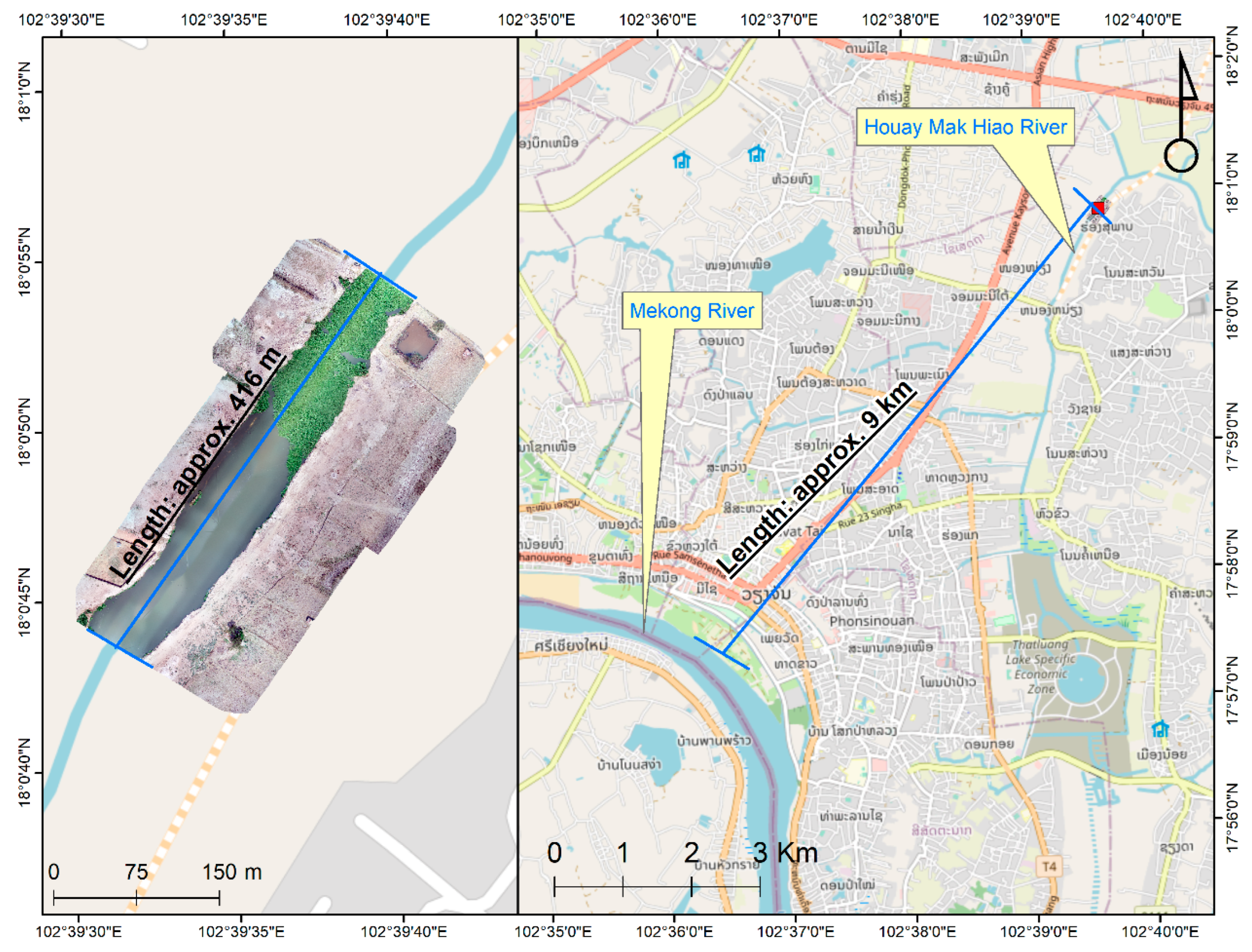
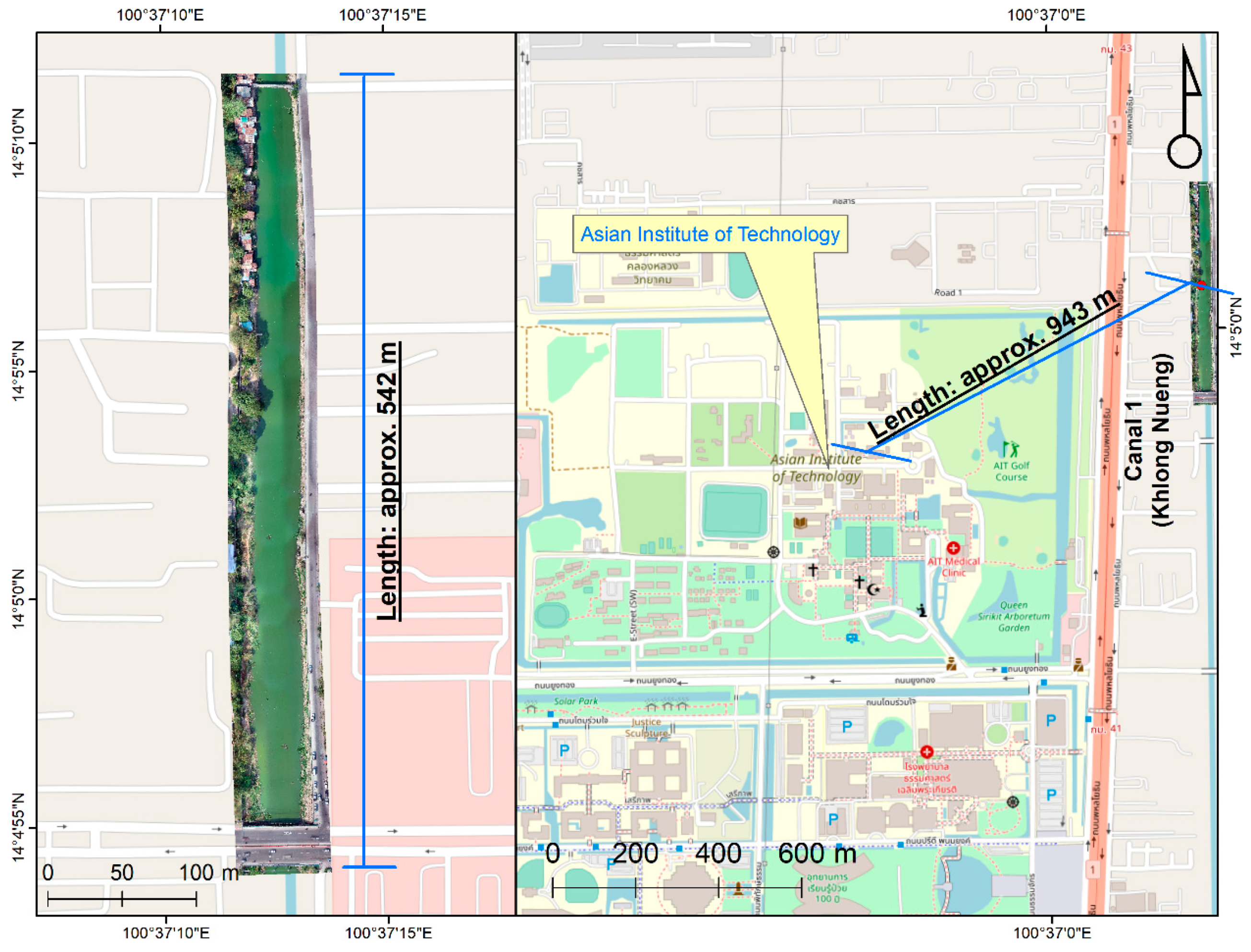
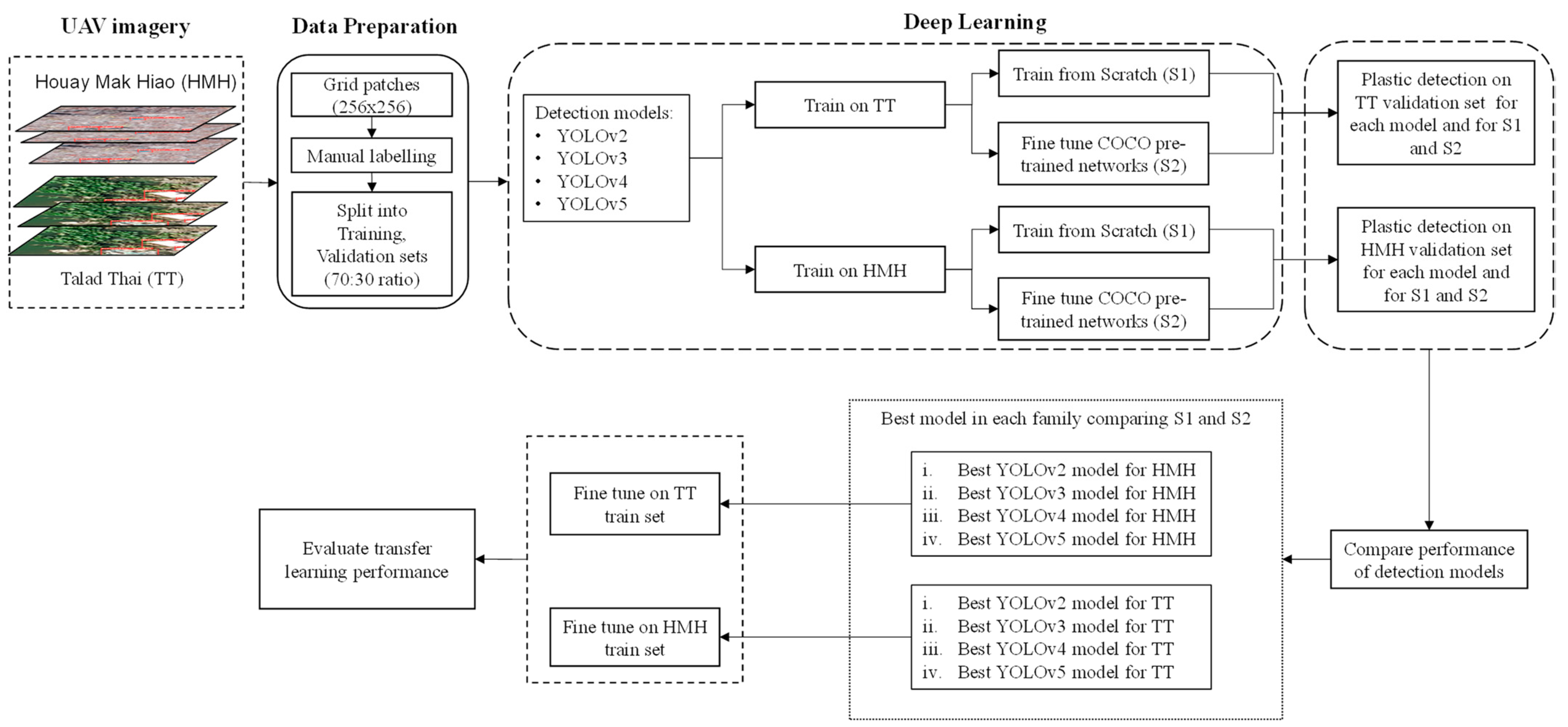
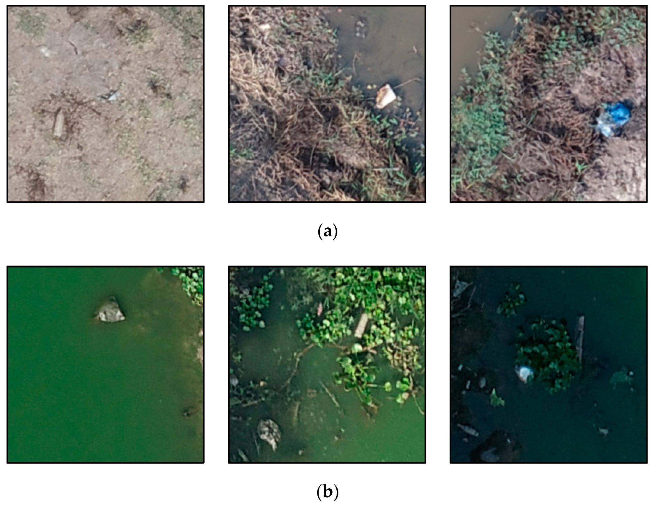
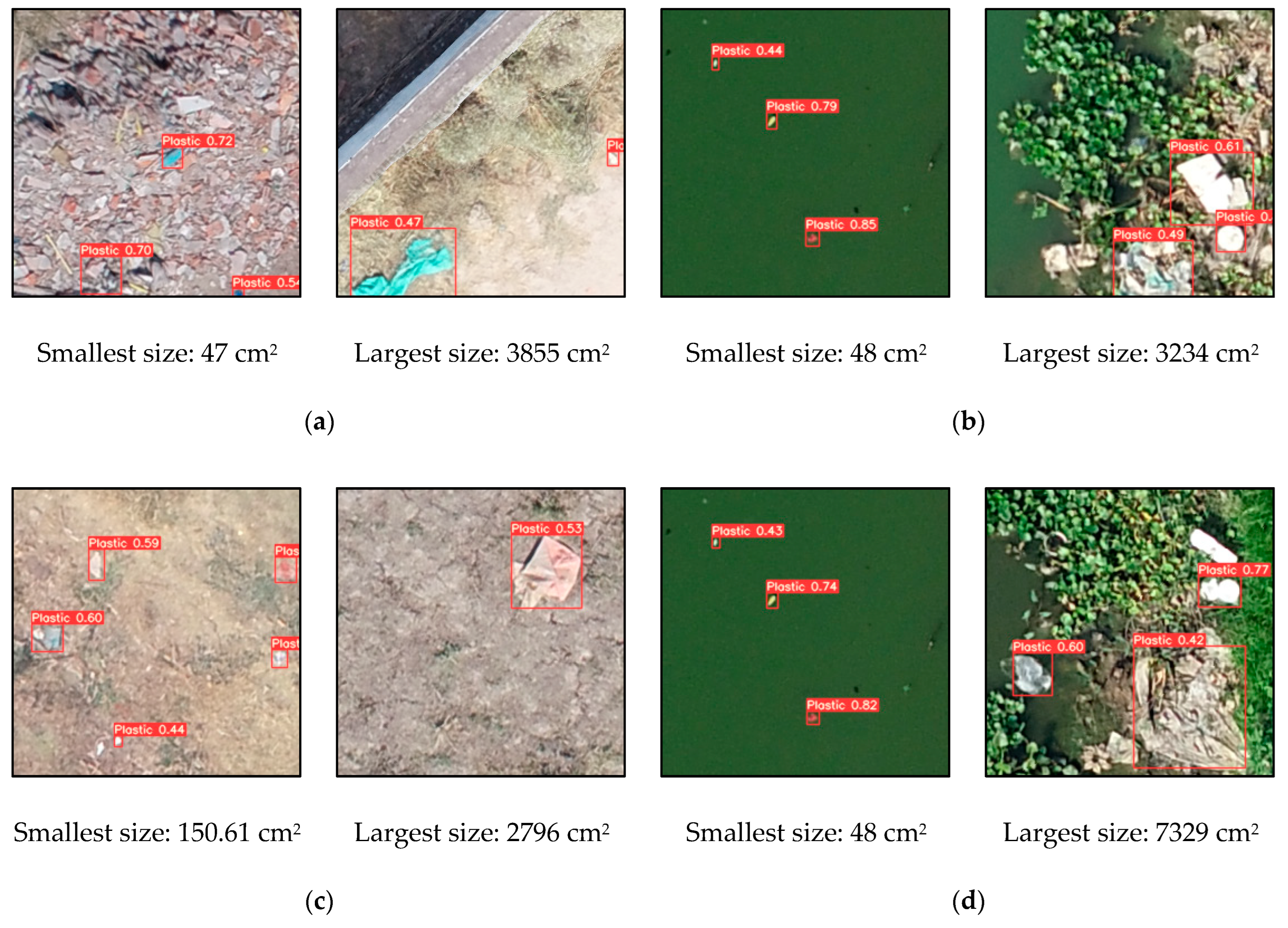
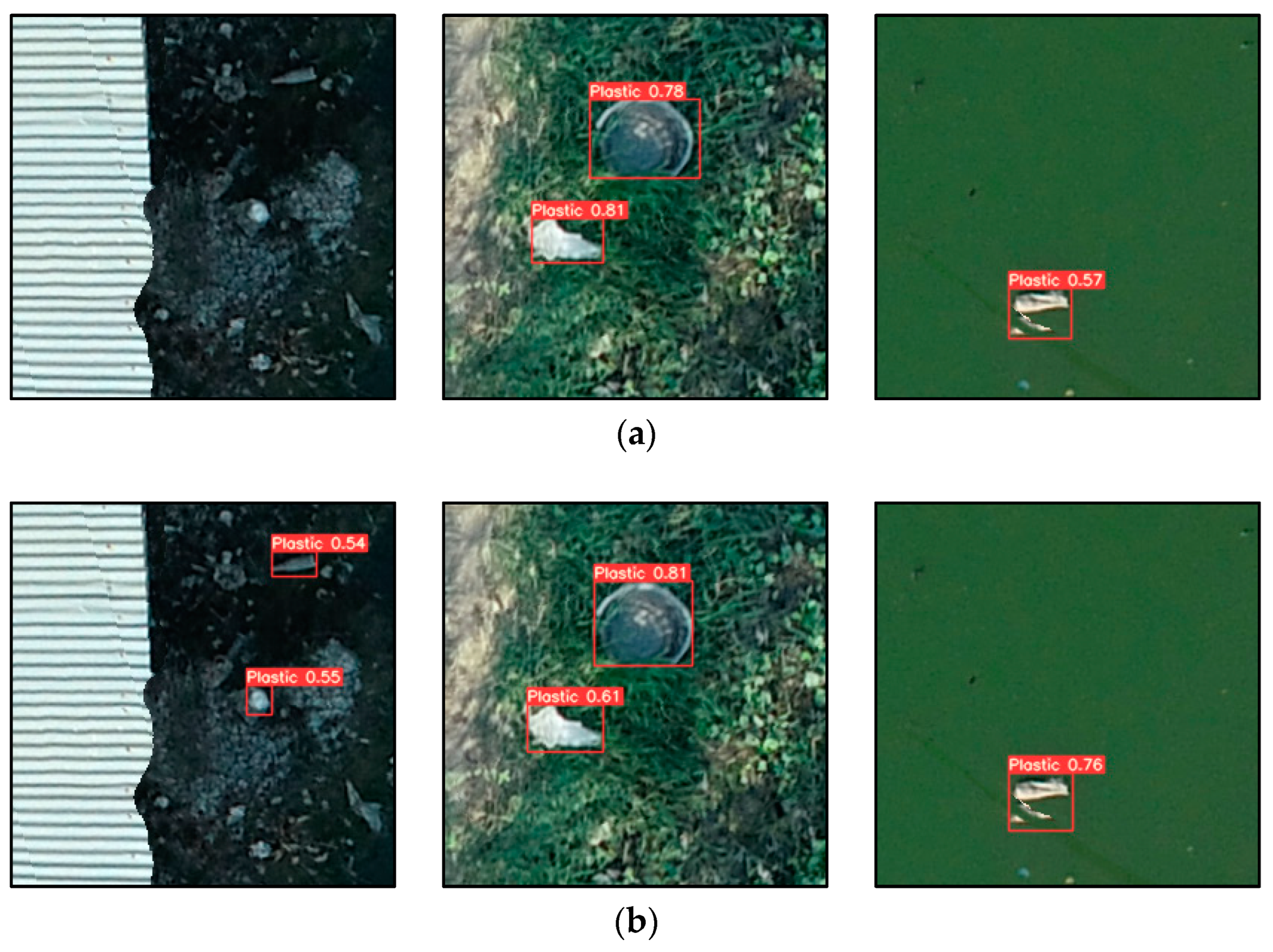
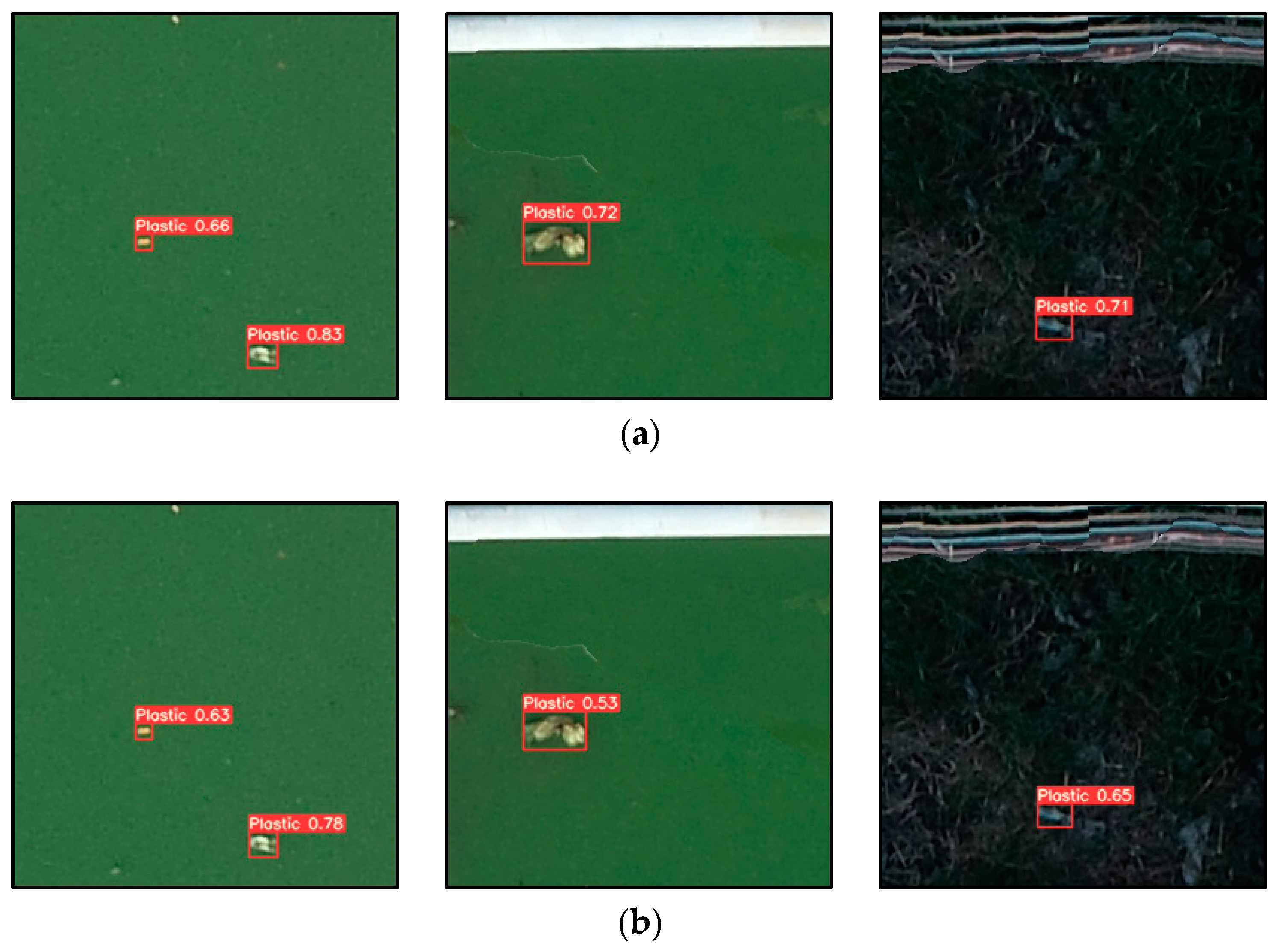
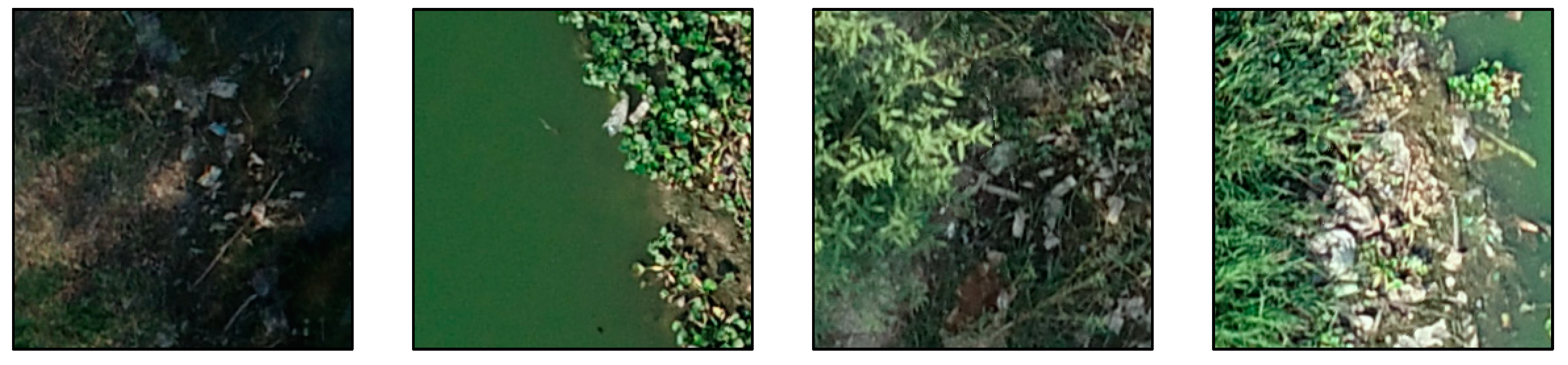
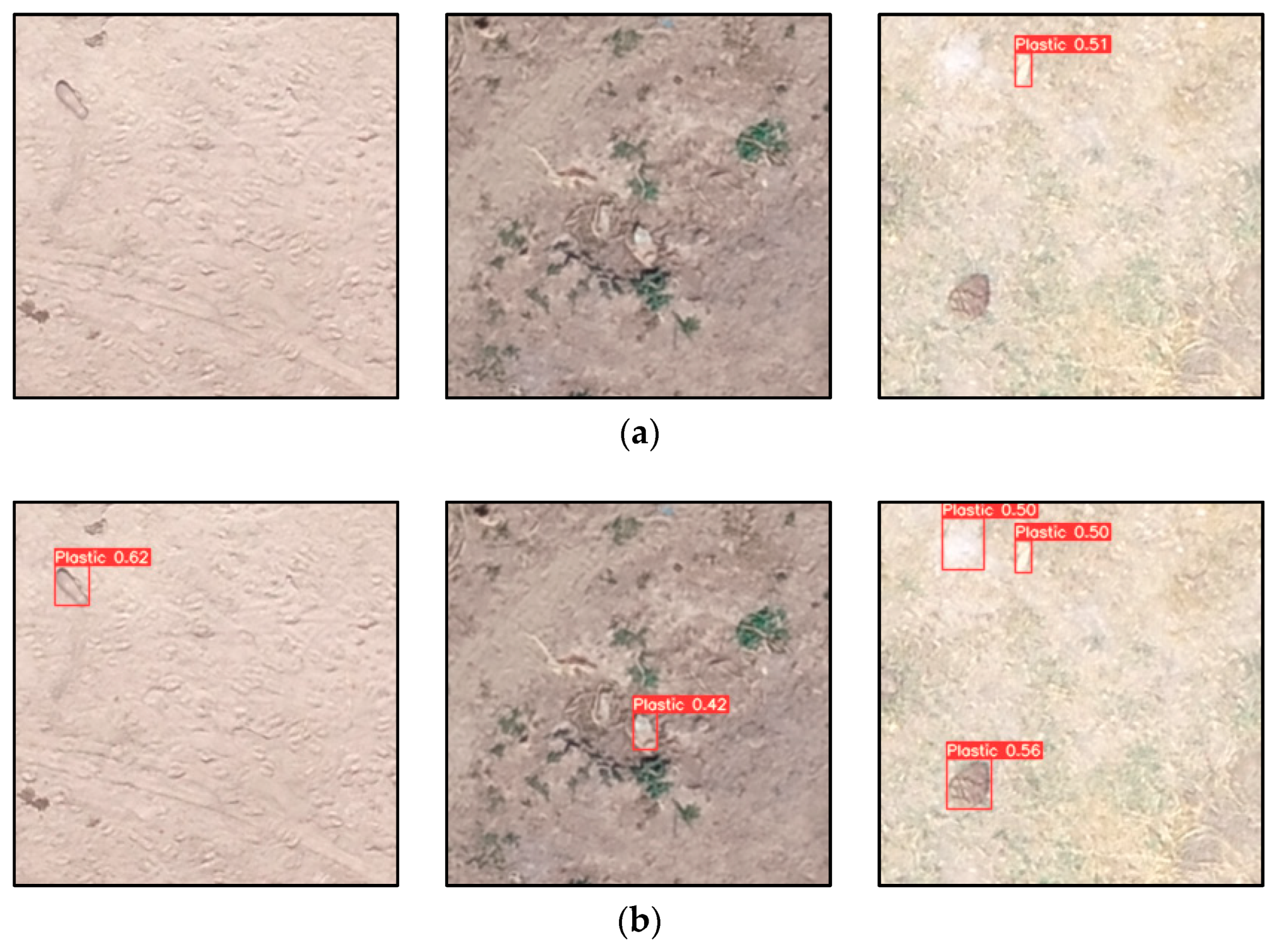
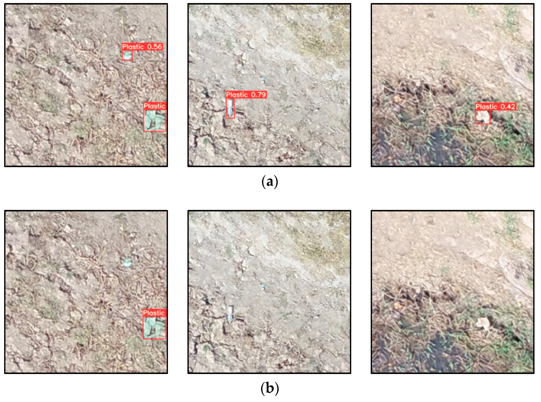
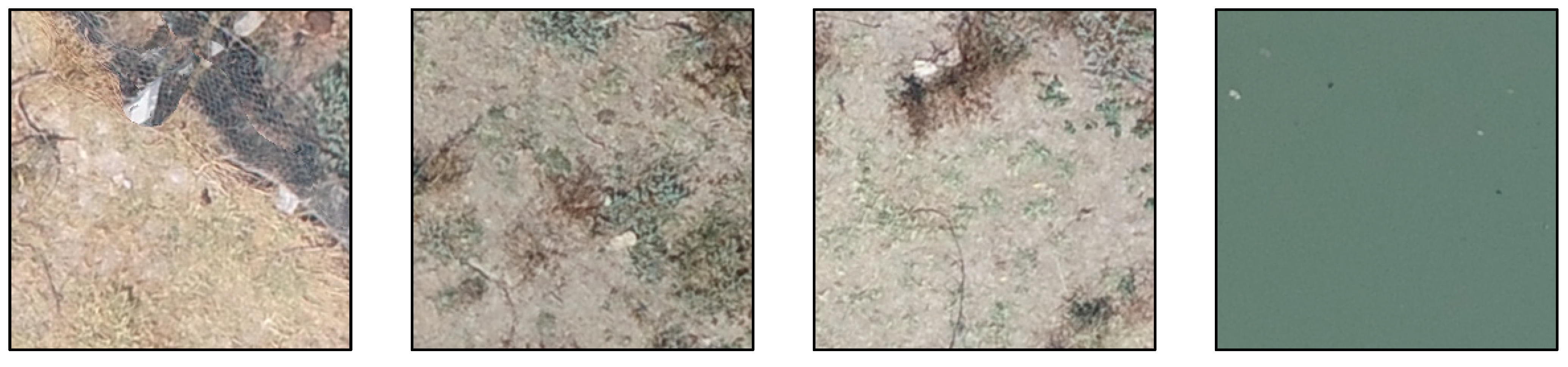
Table 1.
Selection of hyperparameters.
| Parameters | Value |
|---|---|
| Batch size * | 16, 32, 64 and 128 |
| Learning rate | 0.01 to 0.001 |
| No. of filters in YOLO layers | 18 ** |
* YOLOv5 requires a batch size 4 for all experiments due to limited GPU memory; ** Replace number of filters (80 + 5) · 3 for COCO with (1 + 5) · 3 in the convolutional layer before each YOLO layer.
Table 2.
Plastic detection experiment details using Houay Mak Hiao river (HMH) and Khlong Nueng Canal (TT) datasets.
Table 2.
Plastic detection experiment details using Houay Mak Hiao river (HMH) and Khlong Nueng Canal (TT) datasets.
| Experiment | Training Dataset | Testing Dataset | Training Method | Models (YOLO Family) |
|---|---|---|---|---|
| I | HMH | TT | Scratch | YOLOv2 YOLOv2-tiny YOLOv3 YOLOv3-tiny YOLOv3-spp YOLOv4 YOLOv4-tiny YOLOv5s YOLOv5m YOLOv5l YOLOv5x |
| II | Using pre-trained model | |||
| III | TT | HMH | Scratch | |
| IV | Using pre-trained model | |||
| V | HMH | TT | Fine-tuning | YOLOv5s, YOLOv4, YOLOv3-spp, and YOLOv2 trained in II |
| VI | TT | HMH | Fine-tuning | YOLOv5s, YOLOv4, YOLOv3-spp, and YOLOv2 trained in IV |
| VII | Plastic volume estimation using pre-trained YOLOv5s in terms of surface area | |||
Table 3.
Experiment I and II results. Detection Performance on HMH dataset.
| Model | Training Time (h) | Inference Time per Image (s) | Model Size (MB) | Computational Complexity (GFLOPs) | mAP @ 0.5 IoU for Validation Dataset | Map @ 0.5 IoU for Testing Dataset | Highest F1 Score | Computing Platform |
|---|---|---|---|---|---|---|---|---|
| Pre-trained YOLOv2 | 0.359 | 4.74 | 192.9 | 29.338 | 0.723 | 0.442 | 0.66 | Google Colab |
| YOLOv2 scratch | 0.367 | 4.84 | 192.9 | 29.338 | 0.581 | 0.259 | 0.6 | |
| Pre-trained YOLOv2-tiny | 0.166 | 3.53 | 42.1 | 5.344 | 0.467 | 0.293 | 0.38 | |
| YOLOv2-tiny scratch | 0.23 | 3.52 | 42.1 | 5.344 | 0.348 | 0.286 | 0.44 | |
| Pre-trained YOLOv3 tiny | 0.082 | 0.01 | 16.5 | 12.9 | 0.714 | 0.366 | 0.7 | Intel®Core™ i7-10750H CPU @2.60 GHz, 16 GB RAM, and GPU as NVIDIA GeForce RTX 2060 |
| YOLOv3-tiny scratch | 0.082 | 0.004 | 16.5 | 12.9 | 0.555 | 0.336 | 0.58 | |
| Pre-trained YOLOv3 | 0.259 | 0.018 | 117 | 154.9 | 0.735 | 0.396 | 0.72 | |
| YOLOv3 scratch | 0.258 | 0.017 | 117 | 154.9 | 0.479 | 0.311 | 0.54 | |
| Pre-trained YOLOv3-spp | 0.266 | 0.017 | 119 | 155.7 | 0.787 | 0.402 | 0.75 | |
| YOLOv3-spp scratch | 0.279 | 0.014 | 119 | 155.7 | 0.59 | 0.265 | 0.57 | |
| Pre-trained YOLOv4 | 1.884 | 6.85 | 244.2 | 59.563 | 0.809 | 0.463 | 0.78 | Google Colab |
| YOLOv4 scratch | 1.961 | 5.54 | 244.2 | 59.563 | 0.766 | 0.373 | 0.74 | |
| Pre-trained YOLOv4-tiny | 0.899 | 2.92 | 22.4 | 6.787 | 0.758 | 0.418 | 0.76 | |
| YOLOv4-tiny scratch | 0.968 | 2.72 | 22.4 | 6.787 | 0.732 | 0.355 | 0.73 | |
| Pre-trained YOLOv5s | 0.146 | 0.019 | 13.6 | 16.3 | 0.810 | 0.424 | 0.78 | Intel®Core™ i7-10750H CPU @2.60 GHz, 16 GB RAM, and GPU as NVIDIA GeForce RTX 2060 |
| YOLOv5s scratch | 0.149 | 0.017 | 13.6 | 16.3 | 0.740 | 0.272 | 0.67 | |
| Pre-trained YOLOv5m | 0.195 | 0.041 | 40.4 | 50.3 | 0.787 | 0.434 | 0.77 | |
| YOLOv5m scratch | 0.197 | 0.04 | 40.4 | 50.3 | 0.695 | 0.331 | 0.70 | |
| Pre-trained YOLOv5l | 0.265 | 0.027 | 89.3 | 114.1 | 0.810 | 0.422 | 0.78 | |
| YOLOv5l scratch | 0.262 | 0.032 | 89.3 | 114.1 | 0.669 | 0.176 | 0.67 | |
| Pre-trained YOLOv5x | 0.402 | 0.036 | 166 | 217.1 | 0.781 | 0.367 | 0.76 | |
| YOLOv5x scratch | 0.399 | 0.042 | 166 | 217.1 | 0.710 | 0.316 | 0.69 |
Table 4.
Experiment III and IV results. Detection Performance on Talad Thai dataset.
| Model | Training Time (h) | Inference Time per Image (s) | mAP@ 0.5 IoU for Validation Dataset | mAP @ 0.5 IoU for Testing Dataset | Highest F1 Score | Computing Platform |
|---|---|---|---|---|---|---|
| Pre-trained YOLOv2 | 0.649 | 4.74 | 0.499 | 0.452 | 0.52 | Google Colab |
| YOLOv2 scratch | 0.648 | 4.94 | 0.368 | 0.327 | 0.44 | |
| Pre-trained YOLOv2-tiny | 0.162 | 3.53 | 0.328 | 0.256 | 0.33 | |
| YOLOv2-tiny scratch | 0.174 | 3.43 | 0.302 | 0.220 | 0.32 | |
| Pre-trained YOLOv3-tiny | 0.087 | 0.007 | 0.495 | 0.483 | 0.53 | Intel®Core™ i7-10750H CPU @2.60 GHz, 16 GB RAM, and GPU as NVIDIA GeForce RTX 2060 |
| YOLOv3-tiny scratch | 0.088 | 0.007 | 0.409 | 0.562 | 0.47 | |
| Pre-trained YOLOv3 | 0.282 | 0.017 | 0.571 | 0.743 | 0.59 | |
| YOLOv3 scratch | 0.286 | 0.016 | 0.359 | 0.358 | 0.43 | |
| Pre-trained YOLOv3-spp | 0.285 | 0.016 | 0.570 | 0.748 | 0.60 | |
| YOLOv3-spp scratch | 0.28 | 0.016 | 0.390 | 0.511 | 0.41 | |
| Pre-trained YOLOv4 | 1.86 | 4.54 | 0.608 | 0.553 | 0.78 | Google Colab |
| YOLOv4 scratch | 1.89 | 4.63 | 0.544 | 0.524 | 0.75 | |
| Pre-trained YOLOv4-tiny | 0.949 | 2.85 | 0.609 | 0.568 | 0.59 | |
| YOLOv4-tiny scratch | 0.44 | 3.33 | 0.560 | 0.434 | 0.54 | |
| Pre-trained YOLOv5s | 0.146 | 0.029 | 0.610 | 0.767 | 0.61 | Intel®Core™ i7-10750H CPU @2.60 GHz, 16 GB RAM, and GPU as NVIDIA GeForce RTX 2060 |
| YOLOv5s scratch | 0.155 | 0.025 | 0.530 | 0.622 | 0.59 | |
| Pre-trained YOLOv5m | 0.22 | 0.036 | 0.562 | 0.761 | 0.57 | |
| YOLOv5m scratch | 0.221 | 0.036 | 0.426 | 0.494 | 0.49 | |
| Pre-trained YOLOv5l | 0.273 | 0.026 | 0.579 | 0.767 | 0.60 | |
| YOLOv5l scratch | 0.283 | 0.027 | 0.442 | 0.529 | 0.49 | |
| Pre-trained YOLOv5x | 0.41 | 0.035 | 0.575 | 0.779 | 0.57 | |
| YOLOv5x scratch | 0.393 | 0.035 | 0.363 | 0.456 | 0.45 |
Table 5.
Experiment V and VI results. Performance comparison between models trained from scratch, without transfer learning, and with transfer learning by location based on mAP.
Table 5.
Experiment V and VI results. Performance comparison between models trained from scratch, without transfer learning, and with transfer learning by location based on mAP.
| YOLO Family | Best Model (Pre-Trained) | Evaluation Dataset | Mean Average Precision (mAP) | |||
|---|---|---|---|---|---|---|
| Training from Scratch | Pretraining on COCO; No Transfer Learning | Transfer from | Pretraining on COCO + Transfer | |||
| YOLOv5 | YOLOv5s | HMH | 0.74 | 0.81 | TT | 0.83 |
| TT | 0.53 | 0.61 | HMH | 0.62 | ||
| YOLOv4 | YOLOv4 | HMH | 0.76 | 0.80 | TT | 0.83 |
| TT | 0.54 | 0.60 | HMH | 0.61 | ||
| YOLOv3 | YOLOv3-spp | HMH | 0.59 | 0.79 | TT | 0.81 |
| TT | 0.39 | 0.57 | HMH | 0.59 | ||
| YOLOv2 | YOLOv2 | HMH | 0.58 | 0.72 | TT | 0.77 |
| TT | 0.37 | 0.49 | HMH | 0.51 | ||
Publisher’s Note: MDPI stays neutral with regard to jurisdictional claims in published maps and institutional affiliations. |
© 2022 by the authors. Licensee MDPI, Basel, Switzerland. This article is an open access article distributed under the terms and conditions of the Creative Commons Attribution (CC BY) license (https://creativecommons.org/licenses/by/4.0/).
Share and Cite
MDPI and ACS Style
Maharjan, N.; Miyazaki, H.; Pati, B.M.; Dailey, M.N.; Shrestha, S.; Nakamura, T. Detection of River Plastic Using UAV Sensor Data and Deep Learning. Remote Sens. 2022, 14, 3049. https://doi.org/10.3390/rs14133049
AMA Style
Maharjan N, Miyazaki H, Pati BM, Dailey MN, Shrestha S, Nakamura T. Detection of River Plastic Using UAV Sensor Data and Deep Learning. Remote Sensing. 2022; 14(13):3049. https://doi.org/10.3390/rs14133049
Chicago/Turabian StyleMaharjan, Nisha, Hiroyuki Miyazaki, Bipun Man Pati, Matthew N. Dailey, Sangam Shrestha, and Tai Nakamura. 2022. "Detection of River Plastic Using UAV Sensor Data and Deep Learning" Remote Sensing 14, no. 13: 3049. https://doi.org/10.3390/rs14133049
Note that from the first issue of 2016, this journal uses article numbers instead of page numbers. See further details here.