Satellite Imagery to Map Topsoil Organic Carbon Content over Cultivated Areas: An Overview

Abstract

There is a need to update soil maps and monitor soil organic carbon (SOC) in the upper horizons or plough layer for enabling decision support and land management, while complying with several policies, especially those favoring soil carbon storage. This review paper is dedicated to the satellite-based spectral approaches for SOC assessment that have been achieved from several satellite sensors, study scales and geographical contexts in the past decade. Most approaches relying on pure spectral models have been carried out since 2019 and have dealt with temperate croplands in Europe, China and North America at the scale of small regions, of some hundreds of km²: dry combustion and wet oxidation were the analytical determination methods used for 50% and 35% of the satellite-derived SOC studies, for which measured topsoil SOC contents mainly referred to mineral soils, typically cambisols and luvisols and to a lesser extent, regosols, leptosols, stagnosols and chernozems, with annual cropping systems with a SOC value of ~15 g·kg⁻¹ and a range of 30 g·kg⁻¹ in median. Most satellite-derived SOC spectral prediction models used limited preprocessing and were based on bare soil pixel retrieval after Normalized Difference Vegetation Index (NDVI) thresholding. About one third of these models used partial least squares regression (PLSR), while another third used random forest (RF), and the remaining included machine learning methods such as support vector machine (SVM). We did not find any studies either on deep learning methods or on all-performance evaluations and uncertainty analysis of spatial model predictions. Nevertheless, the literature examined here identifies satellite-based spectral information, especially derived under bare soil conditions, as an interesting approach that deserves further investigations. Future research includes considering the simultaneous analysis of imagery acquired at several dates i.e., temporal mosaicking, testing the influence of possible disturbing factors and mitigating their effects fusing mixed models incorporating non-spectral ancillary information.

1. Introduction

Conventional high-resolution soil maps are static and often based on obsolete data in relation to their current application [1,2,3]. Hence, there is an urgent need to update soil map information and monitor soil properties regularly for enabling decision support and land management, while complying with global policies such as the sustainable development goals of United Nations (UN), land neutrality target of the UN Framework Convention on Climate Change—Intergovernmental Panel on Climate Change (UNFCC-IPCC), or the “Caring for Soil” mission of the European Commission [1]. Such monitoring can be carried out either temporally or spatially. This holds especially true in the context of the “4 per 1000” initiative, which necessitates quantifying soil organic carbon (SOC) storage over territories and, hence, spatially estimating and mapping SOC content [2,3]. Indeed, SOC stocks and SOC content display spatial structure at several scales: national scales, e.g., [4,5], as well at the scale of large regions of thousands of km², e.g., [6,7], small regions of hundreds of km², e.g., [8], or even at a farm or field scale, e.g., [9,10]. In the last decades, digital soil mapping (DSM) has been carried out, starting from a number of geo-referenced soil samples analyzed using standard chemical laboratory protocols to construct spatial or geostatistical models, e.g., [11,12]. Multivariate analysis techniques are then used to calibrate a spatial soil property model using geo-referenced soil data available for a limited number of sites and a continuous spatial coverage of covariates including morphometric data, such as elevation and slope, in conjunction with covariates derived from Earth observation such as vegetation indices, especially the Normalized Difference Vegetation Index (NDVI). However, collecting soil samples is time consuming and labor intensive. An alternative approach to gathering SOC information while limiting the number of soil samples collected can rely on Earth observation and proximal measurements [13].

In addition to having spatial structure, soil properties, and particularly SOC, have spectral features in a number of wavelength bands in the visible, near-infrared and shortwave infrared (VNIR-SWIR; 400–2500 nm) [14,15,16]. Such features enable the construction of spectral models, which are models relating soil reflectance with the considered soil property, as already proposed by Huete and Escadafal [17], following earlier studies relating soil colour, soil reflectance and soil properties by Girard [18], Baumgardner et al. [19], Dalal and Henry [20], Escadafal et al. [21] and Henderson et al. [22]. Particularly since the emergence of satellite remote sensing, soil scientists have related the Landsat Thematic Mapper (TM) radiance values to soil properties [21,23]. Since the 1980s, until the advent of satellite time-series with a weekly revisit, relatively few studies related image reflectance values to topsoil SOC content. This domain has increasingly received attention in the last decade.

In the framework of the projects WorldSoils (http://www.world-soils.com/, accessed on 18 May 2022) of the European Space Agency (ESA) and STEROPES of the European Joint H2020 Program SOIL (https://ejpsoil.eu/soil-research/steropes/, accessed on 18 May 2022), both aiming to update SOC maps through pushing forward the use of Sentinel satellite time-series, we aim to review the potential and capabilities as well as the limitations and issues of satellite imagery to map topsoil SOC content over cultivated areas. This review paper is dedicated to the spectrally based approaches that have been achieved from several satellite sensors, study scales and geographical contexts in the past decade.

2. Satellites Spectral Information and Overall Characteristics of Soil Data

To comply with the aim of providing a thorough overview of the literature, we conducted a literature review using the Web of Science database, by applying the query (“soil organic carbon”) AND (“satellite”) searching the field “topic” for all possible years (i.e., from 1991 to early 2022). This query resulted in 632 references. Studies dedicated to grasslands, forests or alpine grasslands were considered non-relevant and removed. The publications dating back to before 1991 were searched through examining the literature cited in the papers older than 1995, and through our own expert knowledge. In all, 62 references were found about satellite-based SOC content prediction, with most of them published in the last three years (Figure 1).

2.1. Satellites Spectral Information

Since 1972, i.e., the very beginning of the civilian satellite remote sensing, until the mid-2010s, satellite data available in the optical domain were mostly acquired from multispectral sensors, i.e., sensors with a discrete number of spectral bands. Most historical data were obtained over wide swaths by the Landsat satellites equipped with Thematic Mapper (TM), Enhanced Thematic Mapper (ETM+), and, more recently, Landsat 8 Operational Land Imager (OLI) sensors with 30 m resolution. Additionally, data from the Satellite Pour l’Observation de la Terre (SPOT) equipped with the sensor Haute Résolution Visible (HRV) with 20 m resolution were found dating back to 1986. Some pioneering studies about topsoil SOC content detection from satellite data have been carried out, for instance, considering SPOT HRV bands [24,25,26] or Landsat bands [27,28,29].

Since 2000, hyperspectral satellite images have been made available from the Hyperion sensor with 30 m resolution onboard the satellite Earth Observing 1 (2000–2017), and from the Compact High-Resolution Imaging Spectrometer (CHRIS) with 17 m resolution onboard the Project for On-Board Autonomy (PROBA-1) micro-satellite (2001–ongoing). Since 2019, the PRecursore IperSpettrale della Missione Applicativa (PRISMA) with 239 spectral bands between 400 and 2505 nm has delivered images with 30 m resolution [30]. Approaches of satellite-based SOC modeling have been carried out from Hyperion [31,32,33], CHRIS-PROBA [34], simulated PRISMA [35] and PRISMA [36]. As the Environmental Mapping and Analysis Program (EnMAP) [37] was just launched on 1 April 2022 and is currently in the commissioning phase, some studies have considered simulated EnMAP for the assessment of SOC content [38,39] till actual EnMAP data becomes available. To our knowledge, no reference was found about simulated spectra for other forthcoming hyperspectral satellites such as CHIME, SHALOM or HypXim. Some recent Chinese studies used the hyperspectral data of the Gaofen-5 satellite with a 30 m resolution and bandwidth of 60 km [40,41,42]. In parallel, with the emerging of precision agriculture, field-scale approaches to SOC modeling have also been developed from satellite sensors with higher spatial resolution: IKONOS with 4 m resolution [43], PlanetScope with 3 m resolution [44] and Worldview 2 with 2.5 m resolution [45,46].

Since 2015 and then 2017, when Sentinel-2A, followed by Sentinel-2B were launched, the Sentinel-2 (S2) time-series equipped with the MultiSpectral Instrument (MSI, 13 spectral bands) provided not only wide spatial coverage over swaths of 290 km, but also 10 to 20 m resolution (10 spectral bands) and a 5-day revisit. The advent of such time-series favored the renewal of the satellite-derived spectral models and particularly for SOC, using either single date acquisitions [44,47,48,49,50,51,52,53,54,55] or multi-date approaches [36,56,57,58,59]. In addition, some authors used Sentinel-1 synthetic aperture radar (SAR) images in their approach, either separately [50,55,58] or directly as covariates within their modeling [55,60]. Over very large areas or at national scales, other authors used coarse resolution satellite series, being either MODIS with 250 or 500 m resolution [61,62] or Sentinel-3 equipped with the Ocean and Land Colour Instrument (OLCI) with 300 m resolution [63].

2.2. Overall Characteristics of Soil Data

2.2.1. Soil Types and Agroecosystems under Study

Most approaches relying on pure spectral models have been carried out since 2019 and have dealt with temperate croplands in Europe, China and North America, with few in Mediterranean [34,35,49,64] and arid environments [29,65,66] and even fewer in tropical ecosystems [27,59,67,68] (Figure 2).

Most studies were in rainfed annual cropping systems with very few studies in vineyards and even fewer in orchards. It should be noted that information on management practices or soil surface conditions was scarce.

Soil types refer to the World Reference Base (WRB) [70] in most cases, although the US Soil Taxonomy [71] was also used. The soils are typically cambisols and luvisols and, to a lesser extent, regosols, leptosols, stagnosols, chernozems and the so-called “inceptisols” of the US Soil Taxonomy (mostly equivalent to cambisols) (Figure 3). The most frequent qualifier is “haplic”. The “calcaric” qualifier is not dominant, and therefore calcium carbonate contents can be assumed to be low.

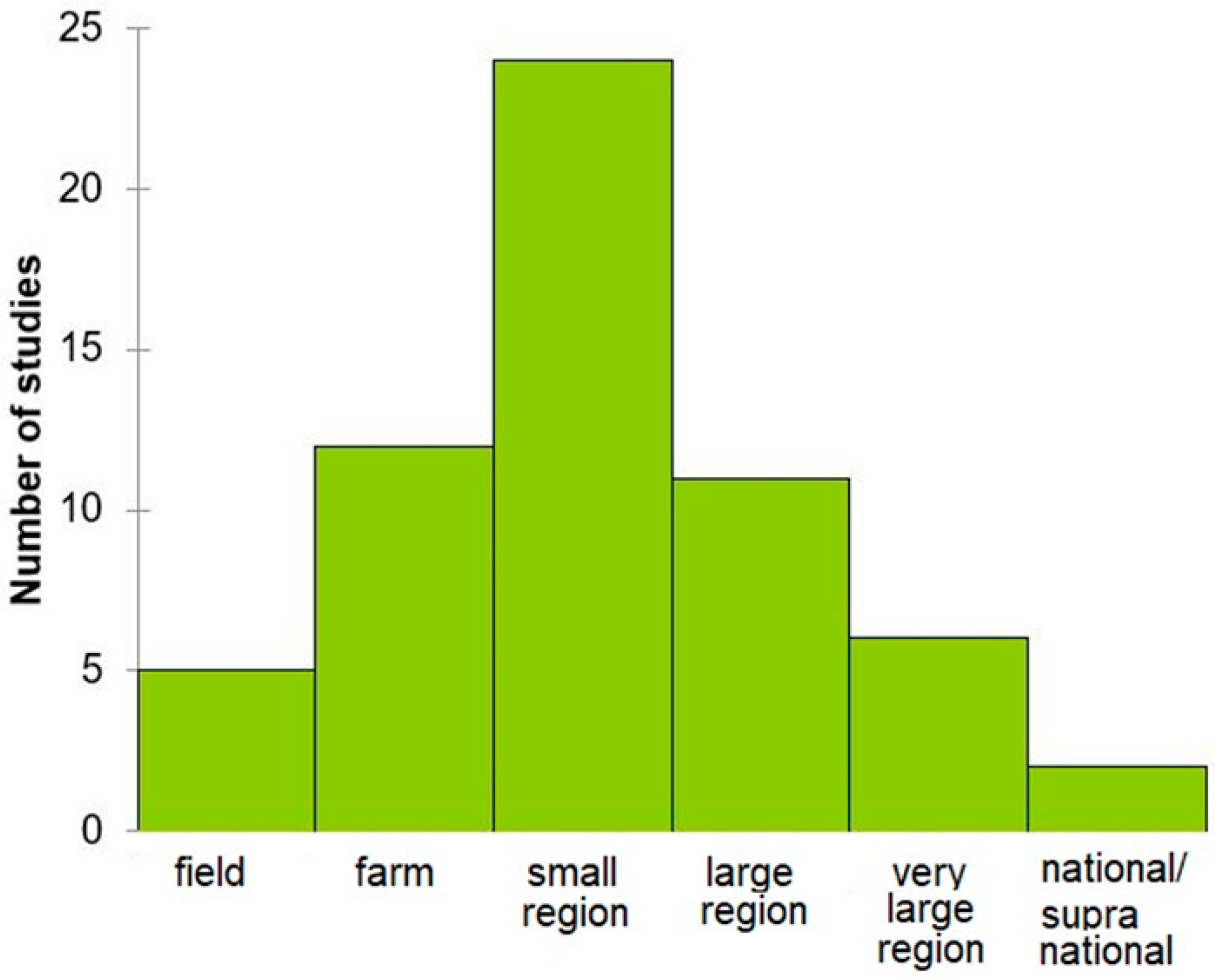
2.2.2. Spatial Scales, Sample Size and Density

Most studies were carried out at the scale of small regions, of some hundreds of km²: study areas covered a median of 118 km² (Figure 4). The sample density for small regions ranged between 0.1 and 16.1 samples per km², with a mean value of 2.7 samples per km². For large regions (up to 10,000 km²) and very large regions (>10,000 km² and up to 150,000 km²), the mean sample density was lower than or equal to 0.1 samples per km², while it was higher than or equal to 201 for farm- or field-scale studies. The total sample size ranged from 32 to 1753 topsoil samples, most of them being collected from the 0–10 cm or 0–20 cm topsoil. The median sample size varies from 85 for field and farm, to 100 for small regions, 264 for large regions and reaches 625 samples for very large regions.

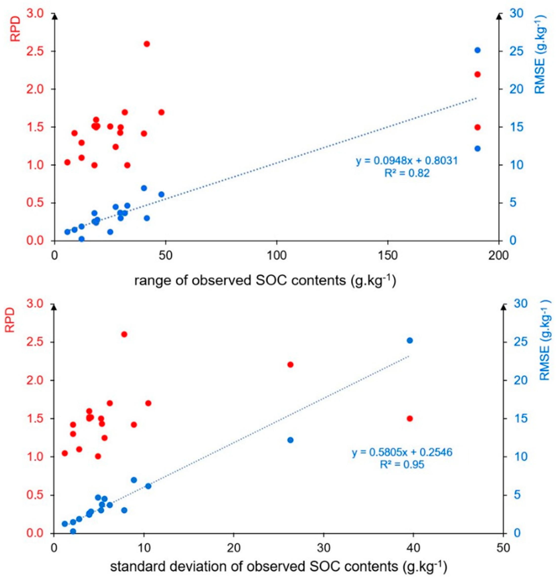
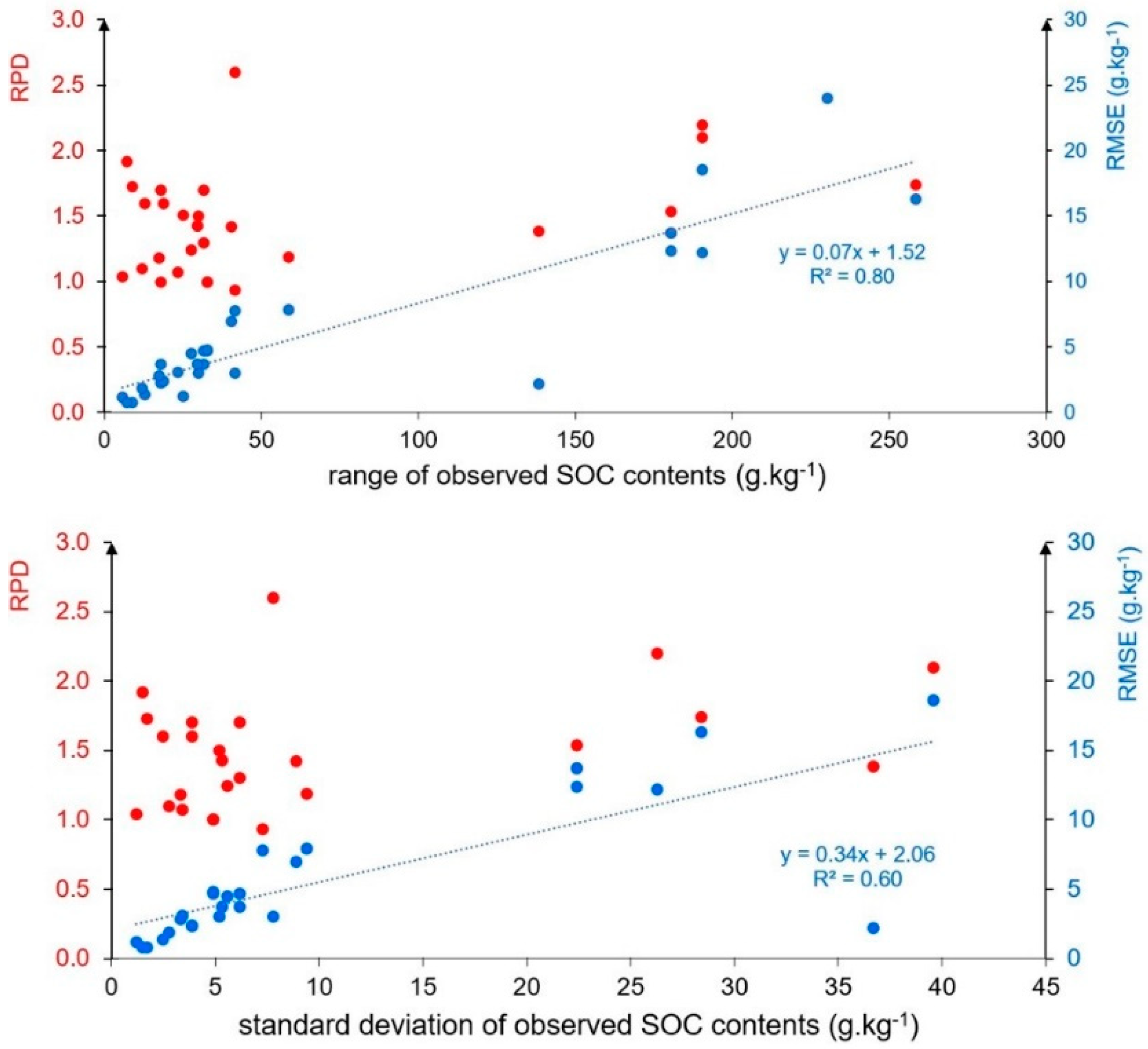
2.2.3. Ranges of SOC Considered and the Issue of Standard Lab Determinations

Table 1. Basics stats of topsoil SOC content values (top SOC, g·kg⁻¹) across 46 study areas with full description of measured sampled sets [18,26,31,34,35,36,41,44,47,48,49,50,52,54,55,57,58,61,64,67,72,73,74,75,76,77,78,79,80,81,82], q1, first quartile; μ, mean; q3; third quartile; σ, standard deviation.

Statistic	Min	q1	µ	q3	Max	σ	Median
Minimum top SOC	0.0	2.7	5.8	6.9	26.1	4.7	6.0
Maximum top SOC	10.0	21.8	82.7	115.8	439.0	102.0	37.3
Top SOC range	4.6	17.8	76.9	110.7	438.4	103.0	30.0
Average top SOC	1.7	12.6	17.4	19.6	50.0	9.5	15.1

sheds light on the basic statistics of topsoil SOC considered in the selected studies. The datasets of measured topsoil SOC contents refer to mineral soils with annual crop systems with an average value of ~15 g·kg⁻¹ and a range of 30 g·kg⁻¹ in median.

Mineral and organic soils are usually processed separately, but the threshold between these categories is not uniform: at the scale of the USA, Wang et al. [83] chose to discriminate between mineral and organic soils using the threshold of 120 g·kg⁻¹.

As the analytical methods used for SOC measurements are far from being homogeneous among laboratories and countries, and specifically in the context of the satellite-derived SOC studies, the basic stats displayed in Table 1 should be considered with caution. Dry combustion was used for 50% of the studies and wet oxidation for 30%, while analytical methods were simply not specified for the remaining studies. Historically, one of the most-used methods has been the Walkley–Black method [84] using wet oxidation. This method is still being used in numerous countries, and several modified methods based on the same principles have also been proposed, e.g., [85,86,87,88]. The underestimation of the total SOC content caused by a reduced wet oxidation of the more stable or “recalcitrant” fractions of SOC is the major limitation of this method.

The modern standard method, supposed to be the reference, is dry combustion coupled with an automated CHN analyzer. Automated dry combustion (ADC) involves measurements of SOC based on CO₂ released from thermally oxidized soil [89]. Therefore, a recovery factor must be used to convert the results from the wet oxidation to the dry combustion method. The most frequently used correction factor is 1.33 [90]. However, a careful look at the literature [90,91,92,93,94] shows that the recovery factors cover a wide range (1 to 1.8) depending on climate, soil types, depth, texture, and the relative proportion of various SOC constituents. Moreover, CN analyzers determine total carbon, i.e., SOC and carbonates. Thus, the SOC content of calcareous samples is determined by subtracting carbon content from carbonates to total carbon content, e.g., [95].

Other standard methods that were not found among the satellite-derived SOC studies include various adaptations of the Mehlich method [96] that aim at extracting humic substances, or loss-on-ignition [89,97], the latter being mainly used for the organic horizons.

All methods have some drawbacks, and the less biased one is ADC, with some exceptions for very organic soils. One consequence is that when using SOC data, and especially when compiling legacy SOC data, metadata should include the laboratory method. Another consequence is that there is no universal factor to convert the results from one method to another, and that such a conversion needs to be locally adapted. Finally, any change of method between two dates may lead to false conclusions about SOC changes.

Moreover, over the past decade, laboratory spectroscopic measurements have been successfully tested to predict SOC contents over the visible near-infrared and shortwave infrared ranges [98,99,100,101], in combination with UV-visible fluorescence measurements [102] or restricted to the visible range only [103], or over the mid-infrared only (4000–400 cm⁻¹) [104]. An emergent technology is also laser-induced breakdown spectroscopy, e.g., [105]. These low-cost technologies are good candidates to provide numerous training information for digital soil mapping (DSM). However, the uncertainty of these measurements often remains a limitation, if the aim is to detect small changes in SOC with time. One emerging promising method is analyzing SOC with Rock-Eval analyses [106], which would pave the way to both estimating total SOC and indicators of its sensibility to mineralization and its potential for long-term sequestration in soils.

3. Approaches Conducted and Their Performances

Studies about SOC prediction from satellites categorize according to four main groups:

(i)

Using spectral information from satellite imagery only, being mostly optical (SPOT, Landsat TM, Hyperion, Landsat 8, Sentinel-2, Pléiades, ASTER); rarely thermal (ASTER);

(ii)

Using spectral information from optical satellite imagery in combination with SAR imagery (e.g., Sentinel-1) or its derived products, such as soil moisture maps;

(iii)

Studies using spectral information from optical satellite imagery in combination with available soil spectral libraries (SSLs) (e.g., open libraries, Land Use and Coverage Area Frame Survey (LUCAS, [107]) for the European Union or the GEOCRADLE (http://datahub.geocradle.eu/dataset/regional-soil-spectral-library, accessed on 18 May 2022) for some Western Mediterranean and Middle Eastern countries), or a local database;

(iv)

Studies using spectral information from optical satellite imagery in combination with non-spectral covariates, such as digital elevation models (DEM).

Group “i” was the most represented, while group “ii” is just emerging [55]. Group “iii“, referred to as a “bottom up” approach by Castaldi et al. [108,109], was developed at the regional scale (e.g., in a loam belt region in Belgium and in the Gutland–Oesling region in Luxembourg [48] and Bavaria (Germany) [74]), at the national scale (e.g., Spain [75]), and then at the supranational, continental scales (e.g., European scale [57,76]) using the LUCAS alone [57,75,76] or in combination with a local database [74,77] and also at the scale of Canada using the CanSYS National Pedon Database [78]. As they are directly derived from the spectral features, we focus on the first three groups.

3.1. Spectral Models Using Spectral Information Only, Combined or Not with Radar

3.1.1. Pretreatments of Image Spectra

So far, various pretreatment methods have been suggested for application to surface reflectance in order to reduce noise and improve the quality of the spectra, i.e., to enhance possible spectral features connected to SOC [110]. In other words, the pretreatment of soil spectra before calibration is needed to diminish the interference or any inappropriate information that cannot be handled correctly by the modeling algorithms [111]. Averaging, centering, smoothing, standardization, normalization and transformation are standard pretreatment practices. For instance, the normalization of the data ensures that the spectral input and the dependent variable have a similar data range [64]. Transformation can be applied to each spectrum individually by subtracting the spectrum mean and scaling with spectrum standard deviation. Almost none of the satellite approaches carried out so far underwent preprocessing, except for those handling hyperspectral images, such as the denoising of PRISMA images [34] or fractional order derivatives (FOD) or discrete wavelet transform (DWT) of Gaofen-5 images [41]. For Gaofen-5 images, Meng et al. [41] used DWT to denoise the original reflectance and derive optimal FOD reflectance. They found that DWT was the optimal technique for denoising spectra prior to predicting soil organic matter. For multispectral satellite images, no pretreatment was carried out except for the spatial filtering of Landsat 5 spectra [74,78]. The centering of a Sentinel-2 reflectance spectrum was preferred, but in the case of a single-date approach only [49]. However, neither log transform nor spectra centering improved prediction performances when several other dates were considered [50].

Another preprocessing method consists of searching and removing outliers from image spectra. An outlier can be defined as an individual that is not consistent with the majority of the data. Therefore, spectral outliers (i.e., samples spectrally different from other samples) in the dataset should be identified and removed. Usually, the Mahalanobis distance [112,113] or Cook’s distance [114,115] can be used for identifying outliers in a dataset. In fact, very few satellite approaches carried out outlier search, and even fewer outlier removal [47,49,55], prior to constructing the SOC prediction models. The main reason for this is the scarcity of samples: even though the initial sample set is large, it might be dramatically reduced after masking in order to only retain the bare soil pixels.

3.1.2. Modeling Approaches and Algorithms

Choosing the most robust calibration method can help to obtain a more reliable prediction model. For satellites with a limited number of spectral bands such as IKONOS, Landsat 1–7, SPOT 1–7 and MODIS, some studies have used means of multiple linear regression (MLR) analysis based on the assumption of a linear relationship between the dependent and independent variables [26,28,43,61,116]. However, most studies have applied multivariate calibration techniques or machine learning algorithms to extract the relevant part of the information for large datasets. Amongst the several multivariate algorithms, partial least squares regression (PLSR) [25,26,31,35,48,49,50,57,58,74] is most widely used and offers the advantage of enabling the understanding of the influence of spectral bands on the SOC prediction. PLSR also has the advantage of being less prone to overfitting when using small sample sets. About one-third of the satellite-derived SOC studies used PLSR, while another third used random forest (RF), and the remaining included MLR, support vector machine (SVM), regression trees such as cubist, and/or kriging. By fitting a PLSR model, one seeks a few PLSR factors that explain most of the variation in both predictors and responses.

RF is another widely-used machine learning technique for SOC modeling [40,48,52,62,75,78]. According to Diaz-Uriarte and de Andrés [117], the most important advantage of RF, which makes it a quite popular choice, is resistance to overfitting and irrelevant features removal. However, this ought to be taken with caution: Wadoux et al. [118] put perfectly irrelevant layers such as the photographs of soil scientists into RF and obtained good overall performances of SOC content prediction. SVM, which is a kernel-based learning algorithm, is another promising method that was successfully used for SOC modeling with satellite-driven data [40,47,52,53]. SVM has been reported by Diaz-Uriarte and de Andrés [117] to return comparable results to RF models. The cubist technique was also applied to satellite images in some recent studies predicting SOC [36,57,59,81]. It is a form of the piecewise linear decision tree that partitions the response data into subsets with which their characteristics are similar with respect to the prediction [101]. Boosting techniques were also considered for modeling purposes. For instance, Zhou et al. [79] used boosted regression tree (BRT), which produces an additive regression model or a tensor product-based approximation, to model SOC using the Sentinel-2 images for the central Alps. In addition, artificial neural network (ANN) has been employed in SOC modeling [64] due to its capability to minimize the learning error in the inverse direction from the output layer towards the input layer.

Currently, deep learning algorithms are increasingly used in image analysis including soil property prediction from satellite images. Deep learning has the capability of processing large-scale and large-dimensional image data [119]. Its advantages over common machine learning techniques are that it supports more sophisticated modeling and permits the easy use of large amounts of computational resources for training such models [120,121]. While common machine learning algorithms tend to plateau in performance after training with a large dataset, deep learning models are expected not only to perform better as the training dataset increases in volume, but also to automatically perform the feature extraction. In a study by Tziolas et al. [64], the convolutional neural network (CNN), as a common deep learning algorithm, was effectively used to combine the complementary information in the pool of both Sentinel-2 and Sentinel-1 over a three-year period and those from auxiliary geographical coordinates to model soil clay. However, literature using deep learning to assess SOC out of satellite data is still scarce, and the techniques often need large datasets (number of samples) to produce stable results not prone to overfitting.

3.1.3. Validation Approaches

Prior to constructing satellite-based SOC spectral models, bare soil pixels must be identified, commonly based on vegetation index thresholding using the Normalized Difference Vegetation Index or NDVI. According to expert knowledge about land use, and sometimes with joint information layers such land use maps, land parcel registers, pixels with NDVI values lower than 0.35 to 0.27, 0.25 or even 0.20 may be retained as bare. While the level of such NDVI threshold does not appear to have a great impact on the SOC prediction performance [50,58], the crucial step of the selection of samples sets vs. validation/evaluation sets depends on such selection process, conditioning their sizes. The sample size decreases in particular when several other indices, such as the NBR2 meant to reduce the effect of dry vegetation residues [77], are used in addition to NDVI. This effect is even stronger in the case of multi-date approaches aiming to produce a temporal mosaic [56,58,122,123].

Provided the bare soil samples are identified, the main series of questions for the selection of samples sets vs. validation/evaluation sets should be:

-

Do you want a global estimate of the performance of your predictions?

-

Do you want an estimate of a global mean or stock in a given area?

-

Do you want to map the uncertainties, and at which spatial resolution?

-

Do you want to know the domain of validity of your predictive model, in the feature and/or in the spatial space?

-

Do you want to address some or all of the above questions?

These questions are generic to all performance evaluations of spatial model predictions. Most of these questions have been discussed in some reference books and papers, e.g., [124,125,126,127,128,129], and there are still debates about the best way to select sample sets for training and/or validation. However, most of the authors agree on the main bad practices that should be avoided, e.g., randomly splitting into a single training and validation set (k-fold splitting should be preferred), using leave-one-out validation when there is a high spatial auto-correlation between observations, not taking clustering of data into account, or applying a model outside of its validity domain [130]. One good practice is to try to cover the feature and spatial spaces as much as possible, both for calibration and validation. Another good practice could be to perform an independent and unbiased sampling, but this practice is often too costly to put in place. A pragmatic trade-off is often “do the best with what you have”. Going further into this discussion is out of the scope of this paper, and would need a dedicated and comprehensive review.

3.1.4. Performances of Purely Spectral Models

Most studies only provided a global estimate of the performance of their predictions, and did not address the above-raised questions. The validation approach was mainly cross-validation, being either leave-one-out or ten-fold, most of the time without prior analysis of the spatial auto-correlation. The most popular performance figures-of-merit for evaluating the quality of model fit were the root mean squared error of cross-validation (RMSE) and the residual prediction deviation (RPD), i.e., the ratio between the standard deviation of the calibration dataset to the RMSE, and/or in some publications, the ratio of performance to interquartile distance (RPIQ_CV) [131], recommended when the distribution of SOC contents is highly skewed. Whatever the model, the magnitude of error increases with the range of SOC contents (Figure 5 and Figure 6), whereas this is not the case for RPD. The magnitude of error also increases with the standard deviation of SOC contents, which confirms a previously observed relationship for proximal sensing [132], although such a relation is weaker here for all models.

The magnitude of error is the highest for national to continental scales, where it typically reaches 15 g·kg⁻¹ or even more, exceeding the observed range of values for single fields or some small homogeneous regions. For a given range of measured SOC contents, the prediction results (e.g., RPD) may vary according to acquisition and soil surface conditions over several dates [50,55,56]. Hence, the temporal variation adds up to the spatial variation. It is worth mentioning that the overwhelming majority of authors used Sentinel-2 images, particularly at the scale of small regions or even smaller pilot zones. For a similarly considered regional area, such as the Versailles Plain, France, with Luvisols from loess and calcic cambisols, Sentinel-2 yielded higher performance than SPOT 4, SPOT 5 with RMSE of c. 3–4 g·kg⁻¹ for Sentinel-2 [49,50,58] compared to >4.5 g·kg⁻¹ for SPOT [26], likely due to greater spectral resolution of Sentinel-2. At the continental scale of Europe, likely due to the greater spatial resolution of the bands in the visible region, a comparison between Sentinel-2 and Landsat 8 results demonstrated the higher capability of the Sentinel-2 sensor in terms of SOC prediction accuracy [57]. In the Chernozem region of Sardice in Southern Moravia (Czech Republic), at a local scale of 1.45 km², very similar prediction accuracy was obtained from Landsat 8 (2.8 g·kg⁻¹) on the one hand, and Sentinel-2 and PlanetScope (2.6 g·kg⁻¹) on the other hand [44].

When the intraregional variance of the measured SOC contents is small, with a range of measured SOC contents of c. 15 g·kg⁻¹, models may not be reliable whatever the acquisition date, with very low RPD values, close to 1 or even less: this was observed for Mediterranean soils in the vineyards of the La Peyne Valley region, France [49], but also for luvisols in Northern Wallonia, Belgium [48], or for paddy soils in Lanxi County, China [80]. In such situations, the spatial structure of the data may be of particular relevance to improve the prediction performance, through mixed models incorporating spectral information into spatial models (see Section 3.3).

3.2. “Bottom-Up” SOC Approaches to Satellite Developed from Soil Spectral Libraries

The so-called “bottom-up” approach [108,109] consists of calibrating spectral models from the laboratory spectra of an SSL at a number of sampling locations; then, the predicted values obtained are used to construct an image-derived spectral model from the satellite pixels being bare at the time of the acquisition. It hence benefits from large datasets obtained in laboratory conditions collected in an SSL. The “spiked bottom-up” approach is a refinement, consisting of considering both an SSL and a local SSL [64], taking advantage of the previously observed benefit of the spiking approach in spectroscopy [98,133]. The bottom-up approach to SOC prediction was initially developed for hyperspectral airborne imagery, such as APEX [109] or AisaFenix [64], and was only recently applied to satellite imagery, Sentinel-2 [57,77], Landsat TM plus ALOS PALSAR [75], Landsat archive [74,76], Landsat 8 [57].

Developed at the scale of the Demmin [77] and Bavaria regions in Germany [74], at the national scale of Spain [75] then at the European scale [57,76], the bottom-up approaches to SOC prediction only used the LUCAS SSL [57,75,76] or spiked with a local database [74,77]. At the scale of Canada, a similar approach relied on the CanSYS National Pedon Database [78], while for the Ha-Ogen plain in Israel, it relied on the GEOCRADLE spectral library [64], the spectra of which were simulated into MSI spectra of Sentinel-2.

According to Castaldi et al. [109], the group “I” (“traditional”) and group “iii” (“bottom-up”) approaches provided very similar estimation accuracy on the independent validation datasets in the case of the Belgium loam belt and Gutland–Oesling region in Luxembourg, but whether such results can be extrapolated to other agro-pedological contexts remains largely unknown.

3.3. Mixed Models Incorporating Spectral Information into Spatial Models

Conventional univariate geostatistical techniques, such as ordinary kriging (OK), generally provide high prediction accuracy for soil properties when a spatial autocorrelation between samples exists for the target variable, thus, if the spatial variability can be explained by a geostatistical model [134]. However, in order to fit valuable spatial models, many samples need to be collected and this aspect makes this kind of approach not always economically feasible, especially for very large areas. In this regard, auxiliary variables (or covariates) strongly correlated to the target variable and available at finer spatial resolution than the average distance between target variable samples can be exploited in geostatistical or mixed (hybrid) models, such as the linear mixed effect model (LMEM), regression kriging (RK), kriging with external drift (KED) or co-kriging (CK). These hybrid models pool two kinds of approaches: deterministic and stochastic, thus combining regression models and the spatial structure of the regression residuals [135]. The deterministic part allows the estimation of the coefficients of the covariates by ordinary least squares, as in the case of RK [34,136], or using other regression or machine learning approaches [82,137,138]. However, contrary to RK, LMEMs with correlated error allow the consideration of the spatial correlation, at the same time estimating the fixed-effect coefficients and the error covariance function parameters by a restricted maximum likelihood (REML) method [139].

Optical sensors on board satellites potentially offer a source of auxiliary variables for soil property estimation. For example, Simbahan et al. [140] estimated soil organic carbon stock using RK, CK and KED models, where IKONOS spectral data were included as covariates combined with other auxiliary variables. In their approach, the spectral data consisted of a single grayscale image computed as the weighted average of the visible bands of a single-date image. Their results showed the advantage of using mixed models including such grayscale image data compared to OK. Other authors successfully applied mixed models, mainly including vegetation indices retrieved from Sentinel-2 [138] or Landsat 7 [82,141]. The primary constraint for applying mixed models is the presence of a spatial structure of the model residuals. Indeed, Aïchi et al. [142], in their attempt to spatialize the soil total carbon (STC) content of their arid study site, showed that the PLS model residuals had a spatial structure and that the approach relying on the RK hybrid method led to more accurate STC content mapping using ASTER satellite images. In contrast, Castaldi et al. [139] did not run the LMEM for SOC estimation due to a lack of a spatial structure of the ordinary least square residuals using Hyperion hyperspectral data. One may easily understand that the presence of spatial autocorrelation may strongly depend on the pixels’ area, the number of field calibration points, the landscape structure and the overall extent of the study area. For instance, if the landscape is composed of very small fields with contrasted soil management practices, a spatial autocorrelation is not plausible. On the contrary, if the fields are very large and include variations in some SOC controlling factors such as, for instance, clay content, a spatial autocorrelation is much more likely to occur. Moreover, in order to observe a real improvement in terms of accuracy compared to non-spatial and univariate geostatistical models, the target variable should be strongly correlated to satellite covariates. On this subject, Li [143] observed how RK models using vegetation indices, retrieved from Landsat 5 imagery, combined with terrain variables did not improve the organic matter estimation compared to OK, and this was probably due to the weak correlation between satellite data and SOC. Because many other factors, not only content variability, affect crop vigor, the correlation strength between soil properties and satellite optical data can be considerably improved using bare soil data instead of vegetation images or indices. It is worth noting that while satellite spatial layers have been used for several years, the overwhelming majority of such layers consisted of single layers of spectral indices calculated on vegetated pixels, or on whatever pixel without any consideration of their soil surface condition. Nevertheless, the physical link between SOC abundance and spectral responses across the electromagnetic spectrum can be fully exploited using bare soil images; thus, the pixels not affected by green or dry vegetation. In this regard, the scarcity of bare soil pixels that may occur at some dates within annual cropping systems [58] might be an issue for capturing the specific spectral influence of bare soils. Another possible issue might be due to the large number of bands of multispectral and hyperspectral sensors that suggest a reduction of the dimensionality before including them in mixed models. This step is strongly advised to avoid multicollinearity and reduce the noise. For this purpose, minimum noise fraction (MNF) and PCA were successfully used respectively for Hyperion bands [139] and for Landsat 7 bands combined with indices [82]. Avoiding multicollinearity and choosing relevant covariates with parsimony for spatial modeling are generic issues, which are not only related to SOC and remote sensing, but to all digital soil mapping (DSM) techniques, e.g., [128,144].

4. Discussion

4.1. Limitations of the Literature Dataset

Regardless of the approach, the literature examined here suggests the large interest of satellite-based spectral information, especially when the soils are bare, and enables the identification of the hot topics to be further addressed and developed using such information (Figure 7).

The accuracy that is yielded through multispectral satellites such as Sentinel-2 can be considered a valuable trade-off compared to hyperspectral airborne acquisitions [44], even more so as Sentinel-2 images are available at no cost. However, only very few papers provided details about surface condition, and even the area extent of bare soil, soil types, date of collection, crop types or crop rotations, management practices, were sometimes not mentioned, making general comparisons difficult. Moreover, as some authors tested one, two or more algorithms on their datasets, the reviewed literature did not enable the comparison of their performances in a systematic manner. For instance, the performance of SOC content prediction, as compared between PLSR and RF, gave similar results for the Demmin sandy region of Germany [48]. It was higher for PLSR compared to RF, with higher RPD values and lower RMSE values for Sardice (Czech Republic) [44], Oesling and Gutland (Luxemburg) [48], and was poorer for the clayey region of Demmin [48] and Bavaria [74] in Germany, as well as for the Guanzhong Plain in China [54]. The reasons why the algorithms perform differently according to regions need to be further examined.

Moreover, the overwhelming majority of satellite-based SOC studies focused on a single acquisition date, yet the performance that may be yielded varies with date [50], and the sample size that can potentially be used increases through a temporal mosaicking considering several dates [58]. In accordance with those needs, computational facilities might be required more often, and all the more when it comes to upscaling from tile to national, and then continental and global scales.

Bottom-up approaches appear very straightforward, as they can benefit from a large SSL, especially at continental scales. However, at the European scale, the models obtained from lab spectra yielded a higher RMSE of ~20.3 g·kg⁻¹ compared to those obtained from the median reflectance value of a three-year time-series of image spectra (RMSE = 16.3 g·kg⁻¹; [57]). This suggests that image reflectance is likely to deliver more realistic information about the pure soil signal. It should be emphasized that small regions, such as Versailles Plain, France (221 km²), have a median SOC content of ~15 g·kg⁻¹ [58] smaller than errors of continental or global SSL-derived models, and very few point locations are represented in such large SSLs (e.g., LUCAS). Hence, another issue referring to spectral model elaboration is rather the availability of soil analyses dating back to a “reasonably recent” period [55], with sufficient spatial density, in the order of one sample per km² or higher. This leads to the questioning of the spatial and spectral representativeness of the soil sample locations, i.e., the sampling design in terms of crop system, crop rotation, soil types and, finally, for a given soil type, in terms of soil management.

Soil management practices are most often not described. For most satellite-based SOC studies, the soil sampling depth relies on an arbitrary cut-off without explicit mention of the assumption of the homogenizing effect by plowing. Nevertheless, crop rotation, fertilization level, organic amendment, conservation tillage practices (no-till or reduced tillage), plowing depth and plowing frequency, in addition to residue input rates and former land use, may influence the vertical gradient of measured SOC content [145,146,147,148,149,150,151]. All such soil management practices impact soil roughness, the presence of dry or green vegetation, and the presence of coarse fragments on the surface. As estimated from Sentinel-1, soil roughness due to plowing at a 30 cm depth was found to have a disturbing impact on Sentinel-2-derived SOC prediction performance, with unpredictable models for autumn and winter dates in the Versailles Plain, France [49]. For the same study region, the highest SOC prediction residuals were observed for the largest coarse fragment percentages [49]. The NBR2 index, also defined by van Deventer et al. [152] as the “Normalized Difference Tillage index” (NDTI) for the Landsat TM, is likely to exclude the spectra of soil covered by straw or crop residues [122] and, because of the proximity between mid-infrared bands and soil moisture absorptions, may also exclude spectra affected by high soil moisture [77]. Minimizing NBR2 values can lead to improved Sentinel-2-based SOC content predictions [56,58,77]. Even finding bare soils is challenging, especially in perennially cropping systems and with an increasing proportion of crop land using conservation or no-tillage systems.

In addition, the consistency between survey area and pixel size or ground sampling distance (GSD) should be examined according to the magnitude of the geometric error and whether topsoil SOC content has a large short-range spatial variability. For the LUCAS survey, a composite topsoil sample is collected within a circle with a 2 m radius, while GSD is as large as 10 or 20 m for Sentinel-2 and 30 m for Landsat 8/9 or many hyperspectral satellites; such discrepancies might explain the lower performance for Landsat [57].

Lastly, as spectral disturbances might be due to the presence of clouds and cloud shadows, the efficiency of atmospheric correction should be accounted for in satellite-based SOC studies. The atmospheric correction has rarely been carried out using synchronous bare soil reflectance measurements in the field [153,154]; however, atmospheric correction models such as ATCOR (the base for the Sen2Cor processor made available by Copernicus for Sentinel-2) are prone to errors, especially in the infrared and SWIR domains [153]. The most frequently used atmospheric correction methods in satellite-based SOC studies were Sen2Cor, MAJA and LaSRC. Gomez et al. [155] carried out such evaluations for clay content and found that the impact of date on model performance was higher than the impact of atmospheric correction models. However, we did not come across a systematic study to assess the impact of these methods on SOC content prediction.

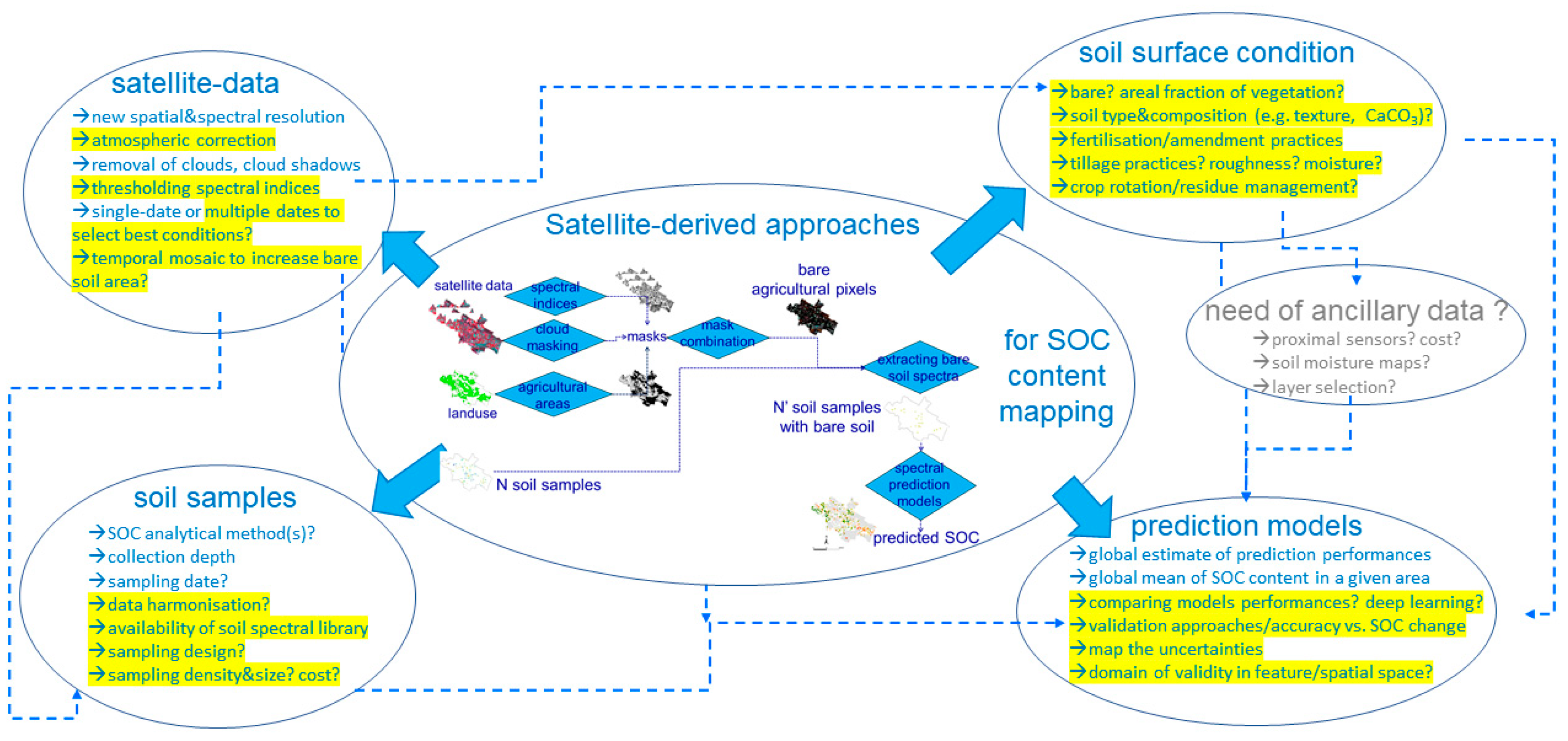
4.2. Future Research Directions

Two critical issues regarding SOC changes in soil are their accounting and their verifiability. The Kyoto Protocol states that sinks and sources of carbon should be accounted for considering uncertainties, transparency in reporting and verifiability. Related to these issues, there are also the incentives or mandatory policies that could favor agricultural practices increasing SOC sequestration at the field or farm level. Further research is to be conducted about the aforementioned disturbing factors that impact the performance of the SOC predictions and, amongst them, soil moisture, the presence of dry and green residues, soil texture and soil salinity are dealt with in the ongoing STEROPES project of the EJP SOIL H2020 program.

Several studies demonstrated that it might be cost-prohibitive to implement systematic sampling to monitor SOC at all farms, e.g., [13,156,157]. This has led to advocating for favoring and monitoring practices that increase SOC, and to use either modeling or IPCC default values, e.g., [158,159,160], to estimate SOC dynamics. However, this option with modeling or using default values to estimate changes is highly questionable, as these default values come from estimates mainly based on the literature, and often on field trials or long-term experiments, the results of which can hardly be extrapolated to farmer fields in different agro-pedo-climatic contexts.

Therefore, it seems reasonable to undertake some real measurements, at least in a subset of representative farms. Stratified design-based sampling, e.g., [161], allows obtaining unbiased estimates of mean values over a given area, together with an estimate of the associated errors. The main questions are how to optimize the location and the areas of the strata and the sampling within each stratum to increase the accuracy of the mean, as well as minimizing the sampling and analytical costs. Several recent studies have shown that using an existing map, even if not perfect, or a sampling strategy based on feature space, allows the optimization of the accuracy of field of farm-scale soil carbon auditing and at the same time decreasing sampling and analysis costs [161,162,163,164].

High-resolution remote sensing predictions have, thus, the potential to help delineate efficient strata, and associated design-based sampling, to conduct low-cost farm-scale carbon auditing on a set of representative farms. This farm-scale carbon auditing would provide objective estimates of changes in order to assess model predictions and/or to locally adapt the IPCC default values.

Together with the facilitation of in situ sampling, satellite-based SOC studies would benefit from considering longer time series in order to (i) retrieve pixels that are temporally representative of the best soil surface conditions for SOC prediction and (ii) increase the bare soil area in optimal condition for SOC prediction. The further handling of ever-longer series should give rise to refined spatio-temporal approaches and the development of groundbreaking approaches such as implying deep learning.

5. Conclusions

The updating of digital soil maps is time consuming and labor intensive. Whatever approach is used, the satellite-based SOC studies that have been published so far suggest significant interest in satellite-based spectral information for such updates, especially for soils that are bare during the acquisition of the satellite image. The accuracy that is yielded through multispectral satellites such as Sentinel-2 can be considered a valuable trade-off compared to hyperspectral airborne acquisitions. The issues that need to be addressed refer to the adequacy of approaches according to agroecosystems and their management practices, in accordance with adequate analytical methods, sampling methods and sampling sizes. The capability to detect SOC changes that are likely to occur due to agricultural management is key for implementing satellite-derived approaches. i.e., for defining the adequate bracket of prediction accuracy and uncertainties. Further studies should better specify such management practices, and in particular those referring to soil cultivation methods.

A careful examination of the possible factors impacting satellite-based SOC models is ongoing and will be implemented together with spatial approaches to sampling, with the possible incorporation of ancillary layers derived from proximal sensing and an intense effort to further promote next-generation hyperspectral satellites, as well as spatio-temporal approaches.

References

1. Tziolas, N.; Tsakiridis, N.; Chabrillat, S.; Demattê, J.A.M.; Ben-Dor, E.; Gholizadeh, A.; Zalidis, G.; van Wesemael, B. Earth Observation Data-Driven Cropland Soil Monitoring: A Review. Remote Sens. 2021, 13, 4439. [Google Scholar] [CrossRef]
2. Minasny, B.; Malone, B.P.; McBratney, A.B.; Angers, D.A.; Arrouays, D.; Chambers, A.; Chaplot, V.; Chen, Z.-S.; Cheng, K.; Das, B.S.; et al. Soil Carbon 4 per Mille. Geoderma 2017, 292, 59–86. [Google Scholar] [CrossRef]
3. Arrouays, D.; Horn, R. Soil Carbon—4 per Mille—An Introduction. Soil Tillage Res. 2019, 188, 1–2. [Google Scholar] [CrossRef]
4. Martin, M.P.; Wattenbach, M.; Smith, P.; Meersmans, J.; Jolivet, C.; Boulonne, L.; Arrouays, D. Spatial Distribution of Soil Organic Carbon Stocks in France. Biogeosciences 2011, 8, 1053–1065. [Google Scholar] [CrossRef] [Green Version]
5. Mulder, V.L.; Lacoste, M.; Richer-de-Forges, A.C.; Martin, M.P.; Arrouays, D. National versus Global Modelling the 3D Distribution of Soil Organic Carbon in Mainland France. Geoderma 2016, 263, 16–34. [Google Scholar] [CrossRef]
6. Poggio, L.; Gimona, A.; Brewer, M.J. Regional scale mapping of soil properties and their uncertainty with a large number of satellite-derived covariates. Geoderma 2013, 209–210, 1–14. [Google Scholar] [CrossRef]
7. Somarathna, P.D.S.N.; Malone, B.P.; Minasny, B. Mapping Soil Organic Carbon Content over New South Wales, Australia Using Local Regression Kriging. Geoderma Reg. 2016, 7, 38–48. [Google Scholar] [CrossRef]
8. Zaouche, M.; Bel, L.; Vaudour, E. Geostatistical Mapping of Topsoil Organic Carbon and Uncertainty Assessment in Western Paris Croplands (France). Geoderma Reg. 2017, 10, 126–137. [Google Scholar] [CrossRef]
9. Crème, A.; Rumpel, C.; Malone, S.L.; Saby, N.P.A.; Vaudour, E.; Decau, M.-L.; Chabbi, A. Monitoring Grassland Management Effects on Soil Organic Carbon—A Matter of Scale. Agronomy 2020, 10, 2016. [Google Scholar] [CrossRef]
10. Poeplau, C.; Bolinder, M.A.; Kätterer, T. Towards an Unbiased Method for Quantifying Treatment Effects on Soil Carbon in Long-Term Experiments Considering Initial within-Field Variation. Geoderma 2016, 267, 41–47. [Google Scholar] [CrossRef]
11. McBratney, A.B.; Mendonça Santos, M.L.; Minasny, B. On Digital Soil Mapping. Geoderma 2003, 117, 3–52. [Google Scholar] [CrossRef]
12. Arrouays, D.; Richer-de-Forges, A.C.; McBratney, A.B.; Hartemink, A.E.; Minasny, B.; Savin, I.; Grundy, M.; Leenaars, J.G.B.; Poggio, L.; Roudier, P.; et al. The Globalsoilmap Project: Past, present, future, and national examples from France. DSB 2018, 95, 3–23. [Google Scholar] [CrossRef]
13. Smith, P.; Soussana, J.; Angers, D.; Schipper, L.; Chenu, C.; Rasse, D.P.; Batjes, N.H.; Egmond, F.; McNeill, S.; Kuhnert, M.; et al. How to Measure, Report and Verify Soil Carbon Change to Realize the Potential of Soil Carbon Sequestration for Atmospheric Greenhouse Gas Removal. Glob. Change Biol. 2020, 26, 219–241. [Google Scholar] [CrossRef] [PubMed] [Green Version]
14. Henderson, T.L.; Szilagyi, A.; Baumgardner, M.F.; Chen, C.T.; Landgrebe, D.A. Spectral Band Selection for Classification of Soil Organic Matter Content. Soil Sci. Soc. Am. J. 1989, 53, 1778–1784. [Google Scholar] [CrossRef]
15. Ben-Dor, E. Quantitative Remote Sensing of Soil Properties. In Advances in Agronomy; Academic Press: Cambridge, MA, USA, 2002; Volume 75, pp. 173–243. ISBN 0065-2113. [Google Scholar]
16. Rasel, S.M.M.; Groen, T.A.; Hussin, Y.A.; Diti, I.J. Proxies for Soil Organic Carbon Derived from Remote Sensing. Int. J. Appl. Earth Observ. Geoinf. 2017, 59, 157–166. [Google Scholar] [CrossRef]
17. Huete, A.R.; Escadafal, R. Assessment of Biophysical Soil Properties through Spectral Decomposition Techniques. Remote Sens. Environ. 1991, 35, 149–159. [Google Scholar] [CrossRef]
18. Girard, M.-C. Emploi de la télédétection pour l’étude de l’humidité des sols. Houille Blanche 1978, 64, 533–539. [Google Scholar] [CrossRef] [Green Version]
19. Baumgardner, M.F.; Silva, L.F.; Biehl, L.L.; Stoner, E.R. Reflectance Properties of Soils. In Advances in Agronomy; Brady, N.C., Ed.; Academic Press: Cambridge, MA, USA, 1986; Volume 38, pp. 1–44. ISBN 0065-2113. [Google Scholar]
20. Dalal, R.C.; Henry, R.J. Simultaneous Determination of Moisture, Organic Carbon, and Total Nitrogen by Near Infrared Reflectance Spectrophotometry. Soil Sci. Soc. Am. J. 1986, 50, 120–123. [Google Scholar] [CrossRef]
21. Escadafal, R.; Girard, M.C.; Courault, D. Modeling the Relationships between Munsell Soil Color and Soil Spectral Properties. In Proceedings of the 5th Symposium of Working Group Remote Sensing, ISSS, Budapest, Hungary, 11–15 April 1988. [Google Scholar]
22. Escadafal, R. Remote Sensing of Arid Soil Surface Color with Landsat Thematic Mapper. Adv. Space Res. 1989, 9, 159–163. [Google Scholar] [CrossRef]
23. Frazier, B.E.; Cheng, Y. Remote Sensing of Soils in the Eastern Palouse Region with Landsat Thematic Mapper. Remote Sens. Environ. 1989, 28, 317–325. [Google Scholar] [CrossRef]
24. Agbu, P.A.; Fehrenbacher, D.J.; Jansen, I.J. Soil Property Relationships with SPOT Satellite Digital Data in East Central Illinois. Soil Sci. Soc. Am. J. 1990, 54, 807–812. [Google Scholar] [CrossRef]
25. Berthier, L.; Pitres, J.C.; Vaudour, E. Prédiction spatiale des teneurs en carbone organique des sols par spectroscopie visible-proche infrarouge et télédétection satellitale SPOT. Exemple au niveau d’un périmètre d’alimentation en eau potable en Beauce. Etude Gest. Sols 2008, 15, 161–172. [Google Scholar]
26. Vaudour, E.; Bel, L.; Gilliot, J.M.; Coquet, Y.; Hadjar, D.; Cambier, P.; Michelin, J.; Houot, S. Potential of SPOT Multispectral Satellite Images for Mapping Topsoil Organic Carbon Content over Peri-Urban Croplands. Soil Sci. Soc. Am. J. 2013, 77, 2122. [Google Scholar] [CrossRef]
27. Nanni, M.R.; Demattê, J.A.M. Spectral Reflectance Methodology in Comparison to Traditional Soil Analysis. Soil Sci. Soc. Am. J. 2006, 70, 393–407. [Google Scholar] [CrossRef]
28. Huang, X.; Senthilkumar, S.; Kravchenko, A.; Thelen, K.; Qi, J. Total carbon mapping in glacial till soils using near-infrared spectroscopy, Landsat imagery and topographical information. Geoderma 2007, 141, 34–42. [Google Scholar] [CrossRef]
29. Jarmer, T.; Hill, J.; Lavée, H.; Sarah, P. Mapping Topsoil Organic Carbon in Non-agricultural Semi-arid and Arid Ecosystems of Israel. Photogramm. Eng. Remote Sens. 2010, 76, 85–94. [Google Scholar] [CrossRef]
30. Loizzo, R.; Guarini, R.; Longo, F.; Scopa, T.; Formaro, R.; Facchinetti, C.; Varacalli, G. Prisma: The Italian hyperspectral mission. In Proceedings of the IGARSS 2018—2018 IEEE International Geoscience and Remote Sensing Symposium, Valencia, Spain, 22–27 July 2018; pp. 175–178. [Google Scholar]
31. Gomez, C.; Viscarra Rossel, R.A.; McBratney, A.B. Soil Organic Carbon Prediction by Hyperspectral Remote Sensing and Field Vis-NIR Spectroscopy: An Australian Case Study. Geoderma 2008, 146, 403–411. [Google Scholar] [CrossRef]
32. Jaber, S.M.; Lant, C.L.; Al-Qinna, M.I. Estimating spatial variations in soil organic carbon using satellite hyperspectral data and map algebra. Int. J. Remote Sens. 2011, 32, 5077–5103. [Google Scholar] [CrossRef]
33. Nowkandeh, S.M.; Homaee, M.; Noroozi, A.A. Mapping Soil Organic Matter Using Hyperion Images. Int. J. Agron. Plant Prod. 2013, 4, 1753–1759. [Google Scholar]
34. Casa, R.; Castaldi, F.; Pascucci, S.; Basso, B.; Pignatti, S. Geophysical and Hyperspectral Data Fusion Techniques for In-Field Estimation of Soil Properties. Vadose Zone J. 2013, 12, 1–10. [Google Scholar] [CrossRef]
35. Castaldi, F.; Palombo, A.; Santini, F.; Pascucci, S.; Pignatti, S.; Casa, R. Evaluation of the potential of the current and forthcoming multispectral and hyperspectral imagers to estimate soil texture and organic carbon. Remote Sens. Environ. 2016, 179, 54–65. [Google Scholar] [CrossRef]
36. Mzid, N.; Castaldi, F.; Tolomio, M.; Pascucci, S.; Casa, R.; Pignatti, S. Evaluation of Agricultural Bare Soil Properties Retrieval from Landsat 8, Sentinel-2 and PRISMA Satellite Data. Remote Sens. 2022, 14, 714. [Google Scholar] [CrossRef]
37. Guanter, L.; Kaufmann, H.; Segl, K.; Foerster, S.; Rogass, C.; Chabrillat, S.; Kuester, T.; Hollstein, A.; Rossner, G.; Chlebek, C.; et al. The EnMAP Spaceborne Imaging Spectroscopy Mission for Earth Observation. Remote Sens. 2015, 7, 8830–8857. [Google Scholar] [CrossRef] [Green Version]
38. Steinberg, A.; Chabrillat, S.; Stevens, A.; Segl, K.; Foerster, S. Prediction of Common Surface Soil Properties Based on Vis-NIR Airborne and Simulated EnMAP Imaging Spectroscopy Data: Prediction Accuracy and Influence of Spatial Resolution. Remote Sens. 2016, 8, 613. [Google Scholar] [CrossRef] [Green Version]
39. Ward, K.J.; Chabrillat, S.; Brell, M.; Castaldi, F.; Spengler, D.; Foerster, S. Mapping Soil Organic Carbon for Airborne and Simulated EnMAP Imagery Using the LUCAS Soil Database and a Local PLSR. Remote Sens. 2020, 12, 3451. [Google Scholar] [CrossRef]
40. Meng, X.; Bao, Y.; Liu, J.; Liu, H.; Zhang, X.; Zhang, Y.; Wang, P.; Tang, H.; Kong, F. Regional soil organic carbon prediction model based on a discrete wavelet analysis of hyperspectral satellite data. Int. J. Appl. Earth Obs. Geoinf. 2020, 89, 102111. [Google Scholar] [CrossRef]
41. Meng, X.; Bao, Y.; Ye, Q.; Liu, H.; Zhang, X.; Tang, H.; Zhang, X. Soil Organic Matter Prediction Model with Satellite Hyperspectral Image Based on Optimized Denoising Method. Remote Sens. 2021, 13, 2273. [Google Scholar] [CrossRef]
42. Bao, Y.; Ustin, S.; Meng, X.; Zhang, X.; Guan, H.; Qi, B.; Liu, H. A Regional-Scale Hyperspectral Prediction Model of Soil Organic Carbon Considering Geomorphic Features. Geoderma 2021, 403, 115263. [Google Scholar] [CrossRef]
43. Sullivan, D.G.; Shaw, J.N.; Rickman, D. IKONOS Imagery to Estimate Surface Soil Property Variability in Two Alabama Physiographies. Soil Sci. Soc. Am. J. 2005, 69, 1789–1798. [Google Scholar] [CrossRef] [Green Version]
44. Žížala, D.; Minařík, R.; Zádorová, T. Soil Organic Carbon Mapping Using Multispectral Remote Sensing Data: Prediction Ability of Data with Different Spatial and Spectral Resolutions. Remote Sens. 2019, 11, 2947. [Google Scholar] [CrossRef]
45. Stamatiadis, S.; Evangelou, L.; Blanta, A.; Tsadilas, C.; Tsitouras, A.; Chroni, C.; Christophides, C.; Tsantila, E.; Samaras, V.; Dalezios, N.; et al. Satellite Visible–Near Infrared Reflectance Correlates to Soil Nitrogen and Carbon Content in Three Fields of the Thessaly Plain (Greece). Commun. Soil Sci. Plant Anal. 2013, 44, 28–37. [Google Scholar] [CrossRef]
46. Samsonova, V.P.; Meshalkina, J.L.; Blagoveschensky, Y.N.; Yaroslavtsev, A.M.; Stoorvogel, J.J. The Role of Positional Errors While Interpolating Soil Organic Carbon Contents Using Satellite Imagery. Precis. Agric. 2018, 19, 1085–1099. [Google Scholar] [CrossRef]
47. Gholizadeh, A.; Žižala, D.; Saberioon, M.; Borůvka, L. Soil organic carbon and texture retrieving and mapping using proximal, airborne and Sentinel-2 spectral imaging. Remote Sens. Environ. 2018, 218, 89–103. [Google Scholar] [CrossRef]
48. Castaldi, F.; Hueni, A.; Chabrillat, S.; Ward, K.; Buttafuoco, G.; Bomans, B.; Vreys, K.; Brell, M.; van Wesemael, B. Evaluating the capability of the Sentinel 2 data for soil organic carbon prediction in croplands. ISPRS J. Photogramm. Remote Sens. 2019, 147, 267–282. [Google Scholar] [CrossRef]
49. Vaudour, E.; Gomez, C.; Fouad, Y.; Lagacherie, P. Sentinel-2 image capacities to predict common topsoil properties of temperate and Mediterranean agroecosystems. Remote Sens. Environ. 2019, 223, 21–33. [Google Scholar] [CrossRef]
50. Vaudour, E.; Gomez, C.; Loiseau, T.; Baghdadi, N.; Loubet, B.; Arrouays, D.; Ali, L.; Lagacherie, P. The Impact of Acquisition Date on the Prediction Performance of Topsoil Organic Carbon from Sentinel-2 for Croplands. Remote Sens. 2019, 11, 2143. [Google Scholar] [CrossRef] [Green Version]
51. Dvorakova, K.; Shi, P.; Limbourg, Q.; van Wesemael, B. Soil Organic Carbon Mapping from Remote Sensing: The Effect of Crop Residues. Remote Sens. 2020, 12, 1913. [Google Scholar] [CrossRef]
52. Zhou, T.; Geng, Y.; Chen, J.; Liu, M.; Haase, D.; Lausch, A. Mapping soil organic carbon content using multi-source remote sensing variables in the Heihe River Basin in China. Ecol. Indic. 2020, 114, 106288. [Google Scholar] [CrossRef]
53. Biney, J.K.M.; Saberioon, M.; Borůvka, L.; Houška, J.; Vašát, R.; Chapman Agyeman, P.; Coblinski, J.A.; Klement, A. Exploring the Suitability of UAS-Based Multispectral Images for Estimating Soil Organic Carbon: Comparison with Proximal Soil Sensing and Spaceborne Imagery. Remote Sens. 2021, 13, 308. [Google Scholar] [CrossRef]
54. Wang, K.; Qi, Y.; Guo, W.; Zhang, J.; Chang, Q. Retrieval and Mapping of Soil Organic Carbon Using Sentinel-2A Spectral Images from Bare Cropland in Autumn. Remote Sens. 2021, 13, 1072. [Google Scholar] [CrossRef]
55. Urbina-Salazar, D.; Vaudour, E.; Baghdadi, N.; Ceschia, E.; Richer-de-Forges, A.C.; Lehmann, S.; Arrouays, D. Using Sentinel-2 Images for Soil Organic Carbon Content Mapping in Croplands of Southwestern France. The Usefulness of Sentinel-1/2 Derived Moisture Maps and Mismatches between Sentinel Images and Sampling Dates. Remote Sens. 2021, 13, 5115. [Google Scholar] [CrossRef]
56. Dvorakova, K.; Heiden, U.; van Wesemael, B. Sentinel-2 Exposed Soil Composite for Soil Organic Carbon Prediction. Remote Sens. 2021, 13, 1791. [Google Scholar] [CrossRef]
57. Castaldi, F. Sentinel-2 and Landsat-8 Multi-Temporal Series to Estimate Topsoil Properties on Croplands. Remote Sens. 2021, 13, 3345. [Google Scholar] [CrossRef]
58. Vaudour, E.; Gomez, C.; Lagacherie, P.; Loiseau, T.; Baghdadi, N.; Urbina-Salazar, D.; Loubet, B.; Arrouays, D. Temporal mosaicking approaches of Sentinel-2 images for extending topsoil organic carbon content mapping in croplands. Int. J. Appl. Earth Obs. Geoinf. 2021, 96, 102277. [Google Scholar] [CrossRef]
59. Silvero, N.E.Q.; Demattê, J.A.M.; Amorim, M.T.A.; dos Santos, N.V.; Rizzo, R.; Safanelli, J.L.; Poppiel, R.R.; de Sousa Mendes, W.; Bonfatti, B.R. Soil Variability and Quantification Based on Sentinel-2 and Landsat-8 Bare Soil Images: A Comparison. Remote Sens. Environ. 2021, 252, 112117. [Google Scholar] [CrossRef]
60. Wang, H.; Zhang, X.; Wu, W.; Liu, H. Prediction of Soil Organic Carbon under Different Land Use Types Using Sentinel-1/-2 Data in a Small Watershed. Remote Sens. 2021, 13, 1229. [Google Scholar] [CrossRef]
61. Dou, X.; Wang, X.; Liu, H.; Zhang, X.; Meng, L.; Pan, Y.; Yu, Z.; Cui, Y. Prediction of soil organic matter using multi-temporal satellite images in the Songnen Plain, China. Geoderma 2019, 356, 113896. [Google Scholar] [CrossRef]
62. Sothe, C.; Gonsamo, A.; Arabian, J.; Snider, J. Large Scale Mapping of Soil Organic Carbon Concentration with 3D Machine Learning and Satellite Observations. Geoderma 2022, 405, 115402. [Google Scholar] [CrossRef]
63. Odebiri, O.; Mutanga, O.; Odindi, J. Deep Learning-Based National Scale Soil Organic Carbon Mapping with Sentinel-3 Data. Geoderma 2022, 411, 115695. [Google Scholar] [CrossRef]
64. Tziolas, N.; Tsakiridis, N.; Ogen, Y.; Kalopesa, E.; Ben-Dor, E.; Theocharis, J.; Zalidis, G. An integrated methodology using open soil spectral libraries and Earth Observation data for soil organic carbon estimations in support of soil-related SDGs. Remote Sens. Environ. 2020, 244, 111793. [Google Scholar] [CrossRef]
65. Jaber, S.M.; Al-Qinna, M.I. Global and local modeling of soil organic carbon using Thematic Mapper data in a semi-arid environment. Arab. J. Geosci. 2015, 8, 3159–3169. [Google Scholar] [CrossRef]
66. Mohamed, E.S.; Baroudy, A.A.E.; El-Beshbeshy, T.; Emam, M.; Belal, A.A.; Elfadaly, A.; Aldosari, A.A.; Ali, A.M.; Lasaponara, R. Vis-NIR Spectroscopy and Satellite Landsat-8 OLI Data to Map Soil Nutrients in Arid Conditions: A Case Study of the Northwest Coast of Egypt. Remote Sens. 2020, 12, 3716. [Google Scholar] [CrossRef]
67. Urbina-Salazar, D.F.; Demattê, J.A.M.; Vicente, L.E.; Guimarães, C.C.B.; Sayão, V.M.; Cerri, C.E.P.; Padilha, M.C.d.C.; Mendes, W.D.S. Emissivity of agricultural soil attributes in southeastern Brazil via terrestrial and satellite sensors. Geoderma 2020, 361, 114038. [Google Scholar] [CrossRef]
68. Silvero, N.E.Q.; Demattê, J.A.M.; de Souza Vieira, J.; de Oliveira Mello, F.A.; Amorim, M.T.A.; Poppiel, R.R.; de Sousa Mendes, W.; Bonfatti, B.R. Soil Property Maps with Satellite Images at Multiple Scales and Its Impact on Management and Classification. Geoderma 2021, 397, 115089. [Google Scholar] [CrossRef]
69. UNESCO. Digital Soil Map of the World; Legend: [Erläuterungen]; UNESCO: Paris, France, 1974; ISBN 978-92-3-101125-2. Available online: https://storage.googleapis.com/fao-maps-catalog-data/uuid/446ed430-8383-11db-b9b2-000d939bc5d8/resources/DSMW.zip (accessed on 13 May 2022).
70. Food and Agriculture Organization of the United Nations. World Reference Base for Soil Resources 2014: International Soil Classification System for Naming Soils and Creating Legends for Soil Maps; FAO: Rome, Italy, 2014; ISBN 978-92-5-108370-3. [Google Scholar]
71. Soil Survey Staff. Soil Taxonomy: A Basic System of Soil Classification for Making and Interpreting Soil Surveys, 2nd ed.; Natural Resources Conservation Service, U.S. Department of Agriculture Handbook; USDA: Washington, DC, USA, 1999; 436p. Available online: https://www.nrcs.usda.gov/wps/portal/nrcs/main/soils/survey/class/taxonomy/ (accessed on 13 May 2022).
72. Liu, T.; Zhang, H.; Shi, T. Modeling and Predictive Mapping of Soil Organic Carbon Density in a Small-Scale Area Using Geographically Weighted Regression Kriging Approach. Sustainability 2020, 12, 9330. [Google Scholar] [CrossRef]
73. Matinfar, H.R.; Maghsodi, Z.; Mousavi, S.R.; Rahmani, A. Evaluation and Prediction of Topsoil organic carbon using Machine learning and hybrid models at a Field-scale. CATENA 2021, 202, 105258. [Google Scholar] [CrossRef]
74. Zepp, S.; Heiden, U.; Bachmann, M.; Wiesmeier, M.; Steininger, M.; van Wesemael, B. Estimation of Soil Organic Carbon Contents in Croplands of Bavaria from SCMaP Soil Reflectance Composites. Remote Sens. 2021, 13, 3141. [Google Scholar] [CrossRef]
75. Wang, X.; Zhang, Y.; Atkinson, P.M.; Yao, H. Predicting soil organic carbon content in Spain by combining Landsat TM and ALOS PALSAR images. Int. J. Appl. Earth Obs. Geoinf. 2020, 92, 102182. [Google Scholar] [CrossRef]
76. Safanelli, J.L.; Chabrillat, S.; Ben-Dor, E.; Demattê, J.A.M. Multispectral Models from Bare Soil Composites for Mapping Topsoil Properties over Europe. Remote Sens. 2020, 12, 1369. [Google Scholar] [CrossRef]
77. Castaldi, F.; Chabrillat, S.; Don, A.; van Wesemael, B. Soil Organic Carbon Mapping Using LUCAS Topsoil Database and Sentinel-2 Data: An Approach to Reduce Soil Moisture and Crop Residue Effects. Remote Sens. 2019, 11, 2121. [Google Scholar] [CrossRef] [Green Version]
78. Sorenson, P.T.; Shirtliffe, S.J.; Bedard-Haughn, A.K. Predictive soil mapping using historic bare soil composite imagery and legacy soil survey data. Geoderma 2021, 401, 115316. [Google Scholar] [CrossRef]
79. Zhou, T.; Geng, Y.; Chen, J.; Pan, J.; Haase, D.; Lausch, A. High-resolution digital mapping of soil organic carbon and soil total nitrogen using DEM derivatives, Sentinel-1 and Sentinel-2 data based on machine learning algorithms. Sci. Total Environ. 2020, 729, 138244. [Google Scholar] [CrossRef] [PubMed]
80. He, X.; Yang, L.; Li, A.; Zhang, L.; Shen, F.; Cai, Y.; Zhou, C. Soil organic carbon prediction using phenological parameters and remote sensing variables generated from Sentinel-2 images. CATENA 2021, 205, 105442. [Google Scholar] [CrossRef]
81. Fathololoumi, S.; Vaezi, A.R.; Alavipanah, S.K.; Ghorbani, A.; Saurette, D.; Biswas, A. Improved digital soil mapping with multitemporal remotely sensed satellite data fusion: A case study in Iran. Sci. Total Environ. 2020, 721, 137703. [Google Scholar] [CrossRef]
82. Mirzaee, S.; Ghorbani-Dashtaki, S.; Mohammadi, J.; Asadi, H.; Asadzadeh, F. Spatial variability of soil organic matter using remote sensing data. CATENA 2016, 145, 118–127. [Google Scholar] [CrossRef]
83. Wang, S.; Guan, K.; Zhang, C.; Lee, D.; Margenot, A.J.; Ge, Y.; Peng, J.; Zhou, W.; Zhou, Q.; Huang, Y. Using Soil Library Hyperspectral Reflectance and Machine Learning to Predict Soil Organic Carbon: Assessing Potential of Airborne and Spaceborne Optical Soil Sensing. Remote Sens. Environ. 2022, 271, 112914. [Google Scholar] [CrossRef]
84. Walkley, A.; Black, I.A. An Examination of the Degtjareff Method for Determining Soil Organic Matter, and a Proposed Modification of the Chromic Acid Titration Method. Soil Sci. 1934, 37, 29–38. [Google Scholar] [CrossRef]
85. Anne, P. Sur le dosage du carbone organique du sol. Ann. Agron. 1945, 15, 161–172. [Google Scholar]
86. Walkley, A. A Critical Examination of a Rapid Method for Determining Organic Carbon in Soils—Effect of Variations in Digestion Conditions and of Inorganic Soil Constituents. Soil Sci. 1947, 63, 251–264. [Google Scholar] [CrossRef]
87. Nelson, D.W.; Sommers, L.E. Total Carbon, Organic Carbon, and Organic Matter. In Methods of Soil Analysis Part 3—Chemical Methods; Sparks, D.L., Page, A.L., Helmke, P.A., Loeppert, R.H., Soltanpour, P.N., Tabatabai, M.A., Johnston, C.T., Summer, M.E., Eds.; Soil Science Society of America: Madison, WI, USA; American Society of Agronomy: Madison, WI, USA, 1996; pp. 961–1010. [Google Scholar]
88. Schumacher, B.A. Methods for the Determination of Total Organic Carbon (TOC) in Soils and Sediments; Ecological Risk Assessment Support Center, U.S. Environmental Protection Agency: Washington, DC, USA, 2002; 23p.
89. Abella, S.R.; Zimmer, B.W. Estimating Organic Carbon from Loss-On-Ignition in Northern Arizona Forest Soils. Soil Sci. Soc. Am. J. 2007, 71, 545–550. [Google Scholar] [CrossRef]
90. Meersmans, J.; Van Wesemael, B.; Van Molle, M. Determining Soil Organic Carbon for Agricultural Soils: A Comparison between the Walkley & Black and the Dry Combustion Methods (North Belgium). Soil Use Manag. 2009, 25, 346–353. [Google Scholar] [CrossRef]
91. Jolivet, C.; Arrouays, D.; Bernoux, M. Comparison between Analytical Methods for Organic Carbon and Organic Matter Determination in Sandy Spodosols of France. Commun. Soil Sci. Plant Anal. 1998, 29, 2227–2233. [Google Scholar] [CrossRef]
92. De Vos, B.; Lettens, S.; Muys, B.; Deckers, J.A. Walkley-Black Analysis of Forest Soil Organic Carbon: Recovery, Limitations and Uncertainty. Soil Use Manag. 2007, 23, 221–229. [Google Scholar] [CrossRef]
93. Chatterjee, A.; Lal, R.; Wielopolski, L.; Martin, M.Z.; Ebinger, M.H. Evaluation of Different Soil Carbon Determination Methods. Crit. Rev. Plant Sci. 2009, 28, 164–178. [Google Scholar] [CrossRef]
94. Roper, W.R.; Robarge, W.P.; Osmond, D.L.; Heitman, J.L. Comparing Four Methods of Measuring Soil Organic Matter in North Carolina Soils. Soil Sci. Soc. Am. J. 2019, 83, 466–474. [Google Scholar] [CrossRef]
95. AFNOR. Qualité des Sols; AFNOR: Paris, France; Eyrolles: Paris, France, 1999; Volume 1, 565p. [Google Scholar]
96. Mehlich, A. Photometric Determination of Humic Matter in Soils, a Proposed Method. Commun. Soil Sci. Plant Anal. 1984, 15, 1417–1422. [Google Scholar] [CrossRef]
97. Ball, D.F. Loss-on-Ignition as an Estimate of Organic Matter and Organic Carbon in Non-Calcareous Soils. J. Soil Sci. 1964, 15, 84–92. [Google Scholar] [CrossRef]
98. Wetterlind, J.; Stenberg, B. Near-Infrared Spectroscopy for within-Field Soil Characterization: Small Local Calibrations Compared with National Libraries Spiked with Local Samples. Eur. J. Soil Sci. 2010, 61, 823–843. [Google Scholar] [CrossRef] [Green Version]
99. Grinand, C.; Barthès, B.G.; Brunet, D.; Kouakoua, E.; Arrouays, D.; Jolivet, C.; Caria, G.; Bernoux, M. Prediction of Soil Organic and Inorganic Carbon Contents at a National Scale (France) Using Mid-Infrared Reflectance Spectroscopy (MIRS). Eur. J. Soil Sci. 2012, 63, 141–151. [Google Scholar] [CrossRef]
100. Gomez, C.; Lagacherie, P.; Coulouma, G. Regional Predictions of Eight Common Soil Properties and Their Spatial Structures from Hyperspectral Vis–NIR Data. Geoderma 2012, 189–190, 176–185. [Google Scholar] [CrossRef]
101. Viscarra Rossel, R.A.; Webster, R. Predicting soil properties from the Australian soil visible–near infrared spectroscopic database. Eur. J. Soil Sci. 2012, 63, 848–860. [Google Scholar] [CrossRef]
102. Vaudour, E.; Cerovic, Z.G.; Ebengo, D.M.; Latouche, G. Predicting Key Agronomic Soil Properties with UV-Vis Fluorescence Measurements Combined with Vis-NIR-SWIR Reflectance Spectroscopy: A Farm-Scale Study in a Mediterranean Viticultural Agroecosystem. Sensors 2018, 18, 1157. [Google Scholar] [CrossRef] [PubMed] [Green Version]
103. Gholizadeh, A.; Saberioon, M.; Viscarra Rossel, R.A.; Boruvka, L.; Klement, A. Spectroscopic Measurements and Imaging of Soil Colour for Field Scale Estimation of Soil Organic Carbon. Geoderma 2020, 357, 113972. [Google Scholar] [CrossRef]
104. Gomez, C.; Chevallier, T.; Moulin, P.; Bouferra, I.; Hmaidi, K.; Arrouays, D.; Jolivet, C.; Barthès, B.G. Prediction of Soil Organic and Inorganic Carbon Concentrations in Tunisian Samples by Mid-Infrared Reflectance Spectroscopy Using a French National Library. Geoderma 2020, 375, 114469. [Google Scholar] [CrossRef]
105. Cremers, D.A.; Ebinger, M.H.; Breshears, D.D.; Unkefer, P.J.; Kammerdiener, S.A.; Ferris, M.J.; Catlett, K.M.; Brown, J.R. Measuring Total Soil Carbon with Laser-Induced Breakdown Spectroscopy (LIBS). J. Environ. Qual. 2001, 30, 2202–2206. [Google Scholar] [CrossRef]
106. Cécillon, L.; Baudin, F.; Chenu, C.; Houot, S.; Jolivet, R.; Kätterer, T.; Lutfalla, S.; Macdonald, A.; van Oort, F.; Plante, A.F.; et al. A Model Based on Rock-Eval Thermal Analysis to Quantify the Size of the Centennially Persistent Organic Carbon Pool in Temperate Soils. Biogeosciences 2018, 15, 2835–2849. [Google Scholar] [CrossRef] [Green Version]
107. Orgiazzi, A.; Ballabio, C.; Panagos, P.; Jones, A.; Fernández-Ugalde, O. LUCAS Soil, the Largest Expandable Soil Dataset for Europe: A Review. Eur. J. Soil Sci. 2018, 69, 140–153. [Google Scholar] [CrossRef] [Green Version]
108. Castaldi, F.; Chabrillat, S.; Chartin, C.; Genot, V.; Jones, A.R.; van Wesemael, B. Estimation of Soil Organic Carbon in Arable Soil in Belgium and Luxembourg with the LUCAS Topsoil Database: Estimation of SOC with the LUCAS Topsoil Database. Eur. J. Soil Sci. 2018, 69, 592–603. [Google Scholar] [CrossRef]
109. Castaldi, F.; Chabrillat, S.; Jones, A.; Vreys, K.; Bomans, B.; van Wesemael, B. Soil Organic Carbon Estimation in Croplands by Hyperspectral Remote APEX Data Using the LUCAS Topsoil Database. Remote Sens. 2018, 10, 153. [Google Scholar] [CrossRef] [Green Version]
110. Gholizadeh, A.; Borůvka, L.; Saberioon, M.M.; Kozák, J.; Vašát, R.; Němeček, K. Comparing Different Data Preprocessing Methods for Monitoring Soil Heavy Metals Based on Soil Spectral Features. Soil Water Res. 2016, 10, 218–227. [Google Scholar] [CrossRef] [Green Version]
111. Coûteaux, M.-M.; Berg, B.; Rovira, P. Near Infrared Reflectance Spectroscopy for Determination of Organic Matter Fractions Including Microbial Biomass in Coniferous Forest Soils. Soil Biol. Biochem. 2003, 35, 1587–1600. [Google Scholar] [CrossRef]
112. Mark, H.L.; Tunnell, D. Qualitative near-infrared reflectance analysis using Mahalanobis distances. Anal. Chem. 1985, 57, 1449–1456. [Google Scholar] [CrossRef]
113. Mark, H. Use of Mahalanobis Distances to Evaluate Sample Preparation Methods for Near-Infrared Reflectance Analysis. Anal. Chem. 1987, 59, 790–795. [Google Scholar] [CrossRef]
114. Cook, R. Detection of influential observation in linear regression. Technometrics 1977, 19, 15–18. [Google Scholar]
115. Kim, M.G. A cautionary note on the use of Cook’s distance. Commun. Stat. Appl. Methods 2017, 24, 317–324. [Google Scholar] [CrossRef] [Green Version]
116. Diek, S.; Fornallaz, F.; Schaepman, M.E. Rogier De Jong Barest Pixel Composite for Agricultural Areas Using Landsat Time Series. Remote Sens. 2017, 9, 1245. [Google Scholar] [CrossRef] [Green Version]
117. Díaz-Uriarte, R.; Alvarez de Andrés, S. Gene Selection and Classification of Microarray Data Using Random Forest. BMC Bioinform. 2006, 7, 3. [Google Scholar] [CrossRef] [PubMed] [Green Version]
118. Wadoux, A.M.J.-C.; Samuel-Rosa, A.; Poggio, L.; Mulder, V.L. A Note on Knowledge Discovery and Machine Learning in Digital Soil Mapping. Eur. J. Soil Sci. 2020, 71, 133–136. [Google Scholar] [CrossRef]
119. LeCun, Y.; Bengio, Y.; Hinton, G. Deep Learning. Nature 2015, 521, 436–444. [Google Scholar] [CrossRef]
120. Behrens, T.; Schmidt, K.; MacMillan, R.A.; Viscarra Rossel, R.A. Multi-Scale Digital Soil Mapping with Deep Learning. Sci. Rep. 2018, 8, 15244. [Google Scholar] [CrossRef] [Green Version]
121. Gholizadeh, A.; Saberioon, M.; Ben-Dor, E.; Viscarra Rossel, R.A.; Borůvka, L. Modelling Potentially Toxic Element in Forest Soils with vis-NIR Spectra and Learning Algorithms. Environ. Pollut. 2020, 267, 115574. [Google Scholar] [CrossRef] [PubMed]
122. Demattê, J.A.M.; Fongaro, C.T.; Rizzo, R.; Safanelli, J.L. Geospatial Soil Sensing System (GEOS3): A Powerful Data Mining Procedure to Retrieve Soil Spectral Reflectance from Satellite Images. Remote Sens. Environ. 2018, 212, 161–175. [Google Scholar] [CrossRef]
123. Rogge, D.; Bauer, A.; Zeidler, J.; Mueller, A.; Esch, T.; Heiden, U. Building an Exposed Soil Composite Processor (SCMaP) for Mapping Spatial and Temporal Characteristics of Soils with Landsat Imagery (1984–2014). Remote Sens. Environ. 2018, 205, 1–17. [Google Scholar] [CrossRef] [Green Version]
124. De Gruijter, J.J.; Bierkens, M.F.P.; Brus, D.J.; Knotters, M. Sampling for Natural Resource Monitoring; Springer: Berlin/Heidelberg, Germany, 2006; ISBN 978-3-540-22486-0. [Google Scholar]
125. Brus, D.J.; Kempen, B.; Heuvelink, G.B.M. Sampling for Validation of Digital Soil Maps. Eur. J. Soil Sci. 2011, 62, 394–407. [Google Scholar] [CrossRef]
126. Lagacherie, P.; Arrouays, D.; Bourennane, H.; Gomez, C.; Nkuba-Kasanda, L. Analysing the Impact of Soil Spatial Sampling on the Performances of Digital Soil Mapping Models and Their Evaluation: A Numerical Experiment on Quantile Random Forest Using Clay Contents Obtained from Vis-NIR-SWIR Hyperspectral Imagery. Geoderma 2020, 375, 114503. [Google Scholar] [CrossRef]
127. Piikki, K.; Wetterlind, J.; Söderström, M.; Stenberg, B. Perspectives on Validation in Digital Soil Mapping of Continuous Attributes—A Review. Soil Use Manag. 2021, 37, 7–21. [Google Scholar] [CrossRef]
128. Wadoux, A.M.J.-C.; Minasny, B.; McBratney, A.B. Machine Learning for Digital Soil Mapping: Applications, Challenges and Suggested Solutions. Earth-Sci. Rev. 2020, 210, 103359. [Google Scholar] [CrossRef]
129. Ploton, P.; Mortier, F.; Réjou-Méchain, M.; Barbier, N.; Picard, N.; Rossi, V.; Dormann, C.; Cornu, G.; Viennois, G.; Bayol, N.; et al. Spatial Validation Reveals Poor Predictive Performance of Large-Scale Ecological Mapping Models. Nat. Commun. 2020, 11, 4540. [Google Scholar] [CrossRef]
130. Wadoux, A.M.J.-C.; Heuvelink, G.B.M.; de Bruin, S.; Brus, D.J. Spatial Cross-Validation Is Not the Right Way to Evaluate Map Accuracy. Ecol. Model. 2021, 457, 109692. [Google Scholar] [CrossRef]
131. Bellon-Maurel, V.; Fernandez-Ahumada, E.; Palagos, B.; Roger, J.-M.; McBratney, A. Critical Review of Chemometric Indicators Commonly Used for Assessing the Quality of the Prediction of Soil Attributes by NIR Spectroscopy. TrAC Trends Anal. Chem. 2010, 29, 1073–1081. [Google Scholar] [CrossRef]
132. Stenberg, B.; Viscarra Rossel, R.A.; Mouazen, A.M.; Wetterlind, J. Visible and Near Infrared Spectroscopy in Soil Science. In Advances in Agronomy; Elsevier: Amsterdam, The Netherlands, 2010; Volume 107, pp. 163–215. ISBN 978-0-12-381033-5. [Google Scholar]
133. Guerrero, C.; Zornoza, R.; Gómez, I.; Mataix-Beneyto, J. Spiking of NIR Regional Models Using Samples from Target Sites: Effect of Model Size on Prediction Accuracy. Geoderma 2010, 158, 66–77. [Google Scholar] [CrossRef]
134. Webster, R.; Oliver, M.A. Geostatistics for Environmental Scientists; Statistics in Practice; Wiley: Hoboken, NJ, USA, 2007; ISBN 978-0-470-51726-0. [Google Scholar]
135. Odeh, I.O.A.; McBratney, A.B.; Chittleborough, D.J. Further Results on Prediction of Soil Properties from Terrain Attributes: Heterotopic Cokriging and Regression-Kriging. Geoderma 1995, 67, 215–226. [Google Scholar] [CrossRef]
136. Hengl, T.; European Commission; Joint Research Centre; Institute for Environment and Sustainability. A Practical Guide to Geostatistical Mapping of Environmental Variables; Office for Official Publications of the European Communities: Luxembourg, 2007; ISBN 978-92-79-06904-8. [Google Scholar]
137. Song, Y.-Q.; Yang, L.-A.; Li, B.; Hu, Y.-M.; Wang, A.-L.; Zhou, W.; Cui, X.-S.; Liu, Y.-L. Spatial Prediction of Soil Organic Matter Using a Hybrid Geostatistical Model of an Extreme Learning Machine and Ordinary Kriging. Sustainability 2017, 9, 754. [Google Scholar] [CrossRef] [Green Version]
138. Pouladi, N.; Møller, A.B.; Tabatabai, S.; Greve, M.H. Mapping Soil Organic Matter Contents at Field Level with Cubist, Random Forest and Kriging. Geoderma 2019, 342, 85–92. [Google Scholar] [CrossRef]
139. Castaldi, F.; Casa, R.; Castrignanò, A.; Pascucci, S.; Palombo, A.; Pignatti, S. Estimation of soil properties at the field scale from satellite data: A comparison between spatial and non-spatial techniques. Eur. J. Soil Sci. 2014, 65, 842–851. [Google Scholar] [CrossRef]
140. Simbahan, G.C.; Dobermann, A.; Goovaerts, P.; Ping, J.; Haddix, M.L. Fine-Resolution Mapping of Soil Organic Carbon Based on Multivariate Secondary Data. Geoderma 2006, 132, 471–489. [Google Scholar] [CrossRef]
141. Song, X.-D.; Brus, D.J.; Liu, F.; Li, D.-C.; Zhao, Y.-G.; Yang, J.-L.; Zhang, G.-L. Mapping Soil Organic Carbon Content by Geographically Weighted Regression: A Case Study in the Heihe River Basin, China. Geoderma 2016, 261, 11–22. [Google Scholar] [CrossRef]
142. Aichi, H.; Fouad, Y.; Lili Chabaane, Z.; Sanaa, M.; Walter, C. Soil Total Carbon Mapping, in Djerid Arid Area, Using ASTER Multispectral Remote Sensing Data Combined with Laboratory Spectral Proximal Sensing Data. Arab. J. Geosci. 2021, 14, 405. [Google Scholar] [CrossRef]
143. Li, Y. Can the Spatial Prediction of Soil Organic Matter Contents at Various Sampling Scales Be Improved by Using Regression Kriging with Auxiliary Information? Geoderma 2010, 159, 63–75. [Google Scholar] [CrossRef]
144. Arrouays, D.; McBratney, A.; Bouma, J.; Libohova, Z.; Richer-de-Forges, A.C.; Morgan, C.L.S.; Roudier, P.; Poggio, L.; Mulder, V.L. Impressions of Digital Soil Maps: The Good, the Not so Good, and Making Them Ever Better. Geoderma Reg. 2020, 20, e00255. [Google Scholar] [CrossRef]
145. Stockfisch, N.; Forstreuter, T.; Ehlers, W. Ploughing Effects on Soil Organic Matter after Twenty Years of Conservation Tillage in Lower Saxony, Germany. Soil Tillage Res. 1999, 52, 91–101. [Google Scholar] [CrossRef]
146. Meersmans, J.; Martin, M.P.; De Ridder, F.; Lacarce, E.; Wetterlind, J.; De Baets, S.; Le Bas, C.; Louis, B.P.; Orton, T.G.; Bispo, A.; et al. A Novel Soil Organic C Model Using Climate, Soil Type and Management Data at the National Scale in France. Agron. Sustain. Dev. 2012, 32, 873–888. [Google Scholar] [CrossRef] [Green Version]
147. Mulder, V.L.; Lacoste, M.; Martin, M.P.; Richer-de-Forges, A.; Arrouays, D. Understanding Large-Extent Controls of Soil Organic Carbon Storage in Relation to Soil Depth and Soil-Landscape Systems: Large-extent controls of SOC storage. Glob. Biogeochem. Cycles 2015, 29, 1210–1229. [Google Scholar] [CrossRef]
148. Metay, A.; Mary, B.; Arrouays, D.; Labreuche, J.; Martin, M.; Nicolardot, B.; Germon, J.-C. Effets des techniques culturales sans labour sur le stockage de carbone dans le sol en contexte climatique tempéré. Can. J. Soil Sci. 2009, 89, 623–634. [Google Scholar] [CrossRef]
149. Noirot-Cosson, P.E.; Vaudour, E.; Gilliot, J.M.; Gabrielle, B.; Houot, S. Modelling the Long-Term Effect of Urban Waste Compost Applications on Carbon and Nitrogen Dynamics in Temperate Cropland. Soil Biol. Biochem. 2016, 94, 138–153. [Google Scholar] [CrossRef]
150. Chenu, C.; Angers, D.A.; Barré, P.; Derrien, D.; Arrouays, D.; Balesdent, J. Increasing Organic Stocks in Agricultural Soils: Knowledge Gaps and Potential Innovations. Soil Tillage Res. 2019, 188, 41–52. [Google Scholar] [CrossRef]
151. Crystal-Ornelas, R.; Thapa, R.; Tully, K.L. Soil Organic Carbon is Affected by Organic Amendments, Conservation Tillage, and Cover Cropping in Organic Farming Systems: A Meta-Analysis. Agric. Ecosyst. Environ. 2021, 312, 107356. [Google Scholar] [CrossRef]
152. Van Deventer, A.P.; Ward, A.D.; Gowda, P.H.; Lyon, G.J. Using Thematic Mapper data to identify contrasting soil plains and tillage practices. Photogramm. Eng. Remote Sens. 1997, 63, 87–93. [Google Scholar]
153. Vaudour, E.; Gilliot, J.M.; Bel, L.; Bréchet, L.; Hamiache, J.; Hadjar, D.; Lemonnier, Y. Uncertainty of Soil Reflectance Retrieval from SPOT and Rapid Eye Multispectral Satellite Images Using a Per-Pixel Bootstrapped Empirical Line Atmospheric Correction over an Agricultural Region. Int. J. Appl. Earth Obs. Geoinf. 2014, 26, 217–234. [Google Scholar] [CrossRef]
154. Vaudour, E.; Gilliot, J.M.; Bel, L.; Lefevre, J.; Chehdi, K. Regional prediction of soil organic carbon content over temperate croplands using visible near-infrared airborne hyperspectral imagery and synchronous field spectra. Int. J. Appl. Earth Obs. Geoinf. 2016, 49, 24–38. [Google Scholar] [CrossRef]
155. Gomez, C.; Vaudour, E.; Féret, J.B.; De Boissieu, F.; Dharumarajan, S. Topsoil clay content mapping from Sentinel-2 data in croplands: Influence of atmospheric correction methods across a season time series. Geoderma 2022, 423, 115959. [Google Scholar] [CrossRef]
156. Smith, P. How Long before a Change in Soil Organic Carbon Can Be Detected?: Time taken to measure a change in soil organic carbon. Glob. Change Biol. 2004, 10, 1878–1883. [Google Scholar] [CrossRef]
157. Smith, P.; Lanigan, G.; Kutsch, W.L.; Buchmann, N.; Eugster, W.; Aubinet, M.; Ceschia, E.; Béziat, P.; Yeluripati, J.B.; Osborne, B.; et al. Measurements Necessary for Assessing the Net Ecosystem Carbon Budget of Croplands. Agric. Ecosyst. Environ. 2010, 139, 302–315. [Google Scholar] [CrossRef]
158. IPCC. Good Practice Guidance for Land Use Change, Land Use Change and Forestry; Institute for Environmental Strategies, Intergovernmental Panel on Climate Change: Hayama, Japan, 2003; Available online: http://www.ipcc-nggip.iges.or.jp/public/gpglulucf/gpglulucf.html (accessed on 13 May 2022).
159. IPCC. IPCC Guidelines for National Greenhouse Gas Inventories; Agriculture Forestry and Other Land Use (AFOLU); Institute for Environmental Strategies, Intergovernmental Panel on Climate Change: Hayama, Japan, 2006; Volume 4, Available online: http://www.ipcc-nggip.iges.or.jp/public/2006gl/index.html (accessed on 13 May 2022).
160. IPCC. 2019 Refinement to the 2006 IPCC Guidelines for National Greenhouse Gas Inventories; Calvo Buendia, E., Tanabe, K., Kranjc, A., Baasansuren, J., Fukuda, M., Ngarize, S., Osako, A., Pyrozhenko, Y., Shermanau, P., Federici, S., Eds.; IPCC: Geneva, Switzerland, 2019; Available online: http://www.ipcc-nggip.iges.or.jp/public/gpglulucf/gpglulucf.html (accessed on 13 May 2022).
161. De Gruijter, J.J.; Minasny, B.; Mcbratney, A.B. Optimizing Stratification and Allocation for Design-Based Estimation of Spatial Means Using Predictions with Error. J. Surv. Stat. Methodol. 2015, 3, 19–42. [Google Scholar] [CrossRef]
162. De Gruijter, J.J.; McBratney, A.B.; Minasny, B.; Wheeler, I.; Malone, B.P.; Stockmann, U. Farm-Scale Soil Carbon Auditing. Geoderma 2016, 265, 120–130. [Google Scholar] [CrossRef]
163. Castaldi, F.; Chabrillat, S.; van Wesemael, B. Sampling Strategies for Soil Property Mapping Using Multispectral Sentinel-2 and Hyperspectral EnMAP Satellite Data. Remote Sens. 2019, 11, 309. [Google Scholar] [CrossRef] [Green Version]
164. Potash, E.; Guan, K.; Margenot, A.; Lee, D.; DeLucia, E.; Wang, S.; Jang, C. How to estimate soil organic carbon stocks of agricultural fields? Perspectives using ex-ante evaluation. Geoderma 2022, 411, 115693. [Google Scholar] [CrossRef]
Figure 1. Histogram of publications of satellite-derived SOC studies according to year.
Remotesensing 14 02917 g001
Figure 2. World map of satellite-derived SOC studies and the dominant soil types of the FAO-UNESCO Digital Soil Map of the World at 1:5.000.000 scale [69]. Time spans are split according to the first year of Sentinel-2 based SOC studies, i.e., 2018.
Remotesensing 14 02917 g002
Figure 3. Word cloud of soil types considered in satellite-derived SOC published studies (word size varies with frequency).
Remotesensing 14 02917 g003
Figure 4. Histogram of study scales considered in satellite-derived SOC studies.
Remotesensing 14 02917 g004
Figure 5. Plot of performance indicators versus range (top) or standard deviation (bottom) of measured SOC contents for PLSR models [26,31,34,36,44,48,49,50,54,55,58,67].
Remotesensing 14 02917 g005
Figure 6. Plot of performance indicators versus range (top) or standard deviation (bottom) of measured SOC contents for all models [18,26,31,34,47,48,49,50,58,74,79,80,81].
Remotesensing 14 02917 g006
Figure 7. Diagram of the main limitations and future research directions referring to satellite-derived approaches for SOC content mapping. Hot topics are underlined in yellow.
Remotesensing 14 02917 g007