Comparative Study of the Es Layer between the Plateau and Plain Regions in China

Abstract

The lower atmosphere forcing plays an important role in forming the sporadic E (Es) layer in the ionosphere. In this study, a comparative study of the Es layer recorded by ionosondes at the middle latitude regions was carried out between the plateau and plain regions in China. The two ionosonde stations (Zhangye, 39.21°N, 100.54°E and Beijing, 40.25°N, 116.25°E) are located at the Qinghai–Tibet Plateau and North China Plain, respectively. The data during the year 2018 were used to reveal the characteristics of the Es layer. The occurrence probability, the critical frequency (foEs) and the base virtual height (h’Es) were considered in this study. Results show that: (1) The diurnal and seasonal variations of the occurrence probability between these two regions are similar. The maximum occurrence probability is at noontime and in the summer season. However, the Es at Zhangye occurred more frequently than Beijing at nighttime and in winter to early spring. (2) Similar to previous studies, the maximum value of foEs at Beijing mainly occurred in summer. Interestingly, the maximum value is in winter at Zhangye station. (3) The characteristics of the anomaly of the Es layer at Zhangye are mostly consistent with the characteristics of atmospheric gravity waves in the Qinghai–Tibet Plateau. Therefore, compared with observations at Beijing, the anomalies of the Es layer at Zhangye (at night and in winter to spring) might be attributed to gravity waves in the lower atmosphere over the Qinghai–Tibet Plateau.

1. Introduction

The sporadic E (Es) layer is a thin layer with high electron density at the altitude of the E layer (90–120 km) in the ionosphere. The thickness of the Es layer is generally 0.6–2.0 km, and its range can reach from dozens to hundreds of kilometers. The lifetime of the Es layer is about 1–8 h [1,2]. Its intensity (the critical frequency or maximum electron density) sometimes can be greater than F-layer peak [3], so the existence of the Es layer has a significant effect on the characteristics of the propagation of radio waves in the ionosphere. The formation mechanism of the Es layer in the mid-latitude region has been mostly attributed to the wind shear theory, which was first proposed and formulated by Whitehead [4] and Axford [5] and further developed afterwards [6,7]. The wind shear theory suggests that the vertical ion convergence driven by the vertical shear in the horizontal neutral wind can compress ions and molecules into a thin layer of metal ions and molecular ions within a range of 90 to 120 km. Generally, tidal waves, gravity waves and planetary waves (PW) play an important role in controlling the occurrence and intensity of the Es layer in mid-latitude region [8,9,10,11,12,13,14].

Previous studies suggest that there are some typical diurnal and seasonal characteristics for the Es layer. Arras et.al [15] used GPS radio occultation measurements from CHAMP, GRACE-A and FORMOSAT-3/COSMIC to obtain the global distribution of the Es layers. Additionally, the results show strong seasonal variations with the highest occurrence rates of the Es layer during summer in the middle latitudes. Haldoupis et al. [16] studied the relationship between the foEs and the annual variation of the sporadic meteor deposition in the mid-latitude region. They found that the intensity of the Es layer in those mid-latitude regions show typical summer maximum characteristics, and the pronounced seasonal dependence of the Es layer has a good correlation with the annual variation of sporadic meteor deposition in the upper atmosphere. Therefore, the atmospheric deposition of meteors might be used to explain the maximum of the Es layer occurring in summer.

In addition, the Es layer is also closely correlated with the sporadic metal layer. Dou et al. [17] explored the features of sporadic sodium layers (SSSLs) and thermospheric-enhanced sodium layers (TeSLs) by a lidar chain over China (Beijing (40.2°N, 116.2°E), Hefei (31.8°N, 117.3°E), Wuhan (30.5°N, 114.4°E) and Haikou (19.5°N, 109.1°E)). They found that both the SSLs and TeSLs at four lidar sites correlated well with Es layer. The research of Williams et al. [18] also confirmed it by using the sporadic sodium and sporadic E layers observed at CO (40.6°N, 105°W) and Utah (41.9°N, 111.4°W).

Pietrella and Bianchi [19] used ionospheric observations from the Roman Ionospheric Observatory during January 1976 and December 2007 to analyze the Es layer. Results show that the occurrence of the Es layer is relatively low in each season before sunrise and after sunset, and the maximum occurrence of the Es layer is during the daytime in summer. In addition, the Es layer seemingly has no correlation with solar and geomagnetic activities. Yu et al. [20] reported that the long-term climatology of the intensity of the Es layer based on the S4 max data retrieved from the COSMIC GPS radio occultation during December 2006 and January 2014. The global Es map shows that the maximum intensity of the Es layer occurred in the mid-latitude region and the intensity in summer is 2 to 3 times higher than winter. On the other hand, Pietrella et al. [21] conducted a comparative Es layer study between two mid-latitude stations, Rome (Italy, 41.8°N, 12.5°E) and Gibilmanna (Italy, 37.9°N, 14.0°E). Due to the closer distance between the two stations, there is a high probability that the Es layer also exists over Gibilmanna when an Es layer occurs at Rome. It is worth noting that what they emphasized is the relationship between the Es layer over Rome and Gibilmanna. In addition, Pietrella et al. [21] found that there are no significant dependences on solar activity for the occurrence of the Es layer at these two middle stations.

Although the diurnal, seasonal and spatial variabilities of the Es have been investigated in many studies in the mid-latitude region, it is worth studying the characteristics of the Es layer, especially for the coupling of the Es layer and lower atmosphere. It helps us fully understand the formation of the Es layer in the ionosphere. In this study, a comparative study of the Es layer between two kinds of the topography in the mid-latitude regions was carried out. One station is located at Beijing in North China plain, the other station is located at Zhangye, sitting on the edge of the Qinghai–Tibet Plateau. The ionospheric parameter obtained from the two ionosondes covering the whole year of 2018. The comparative study of the Es layer could help reveal its characteristics from another perspective.

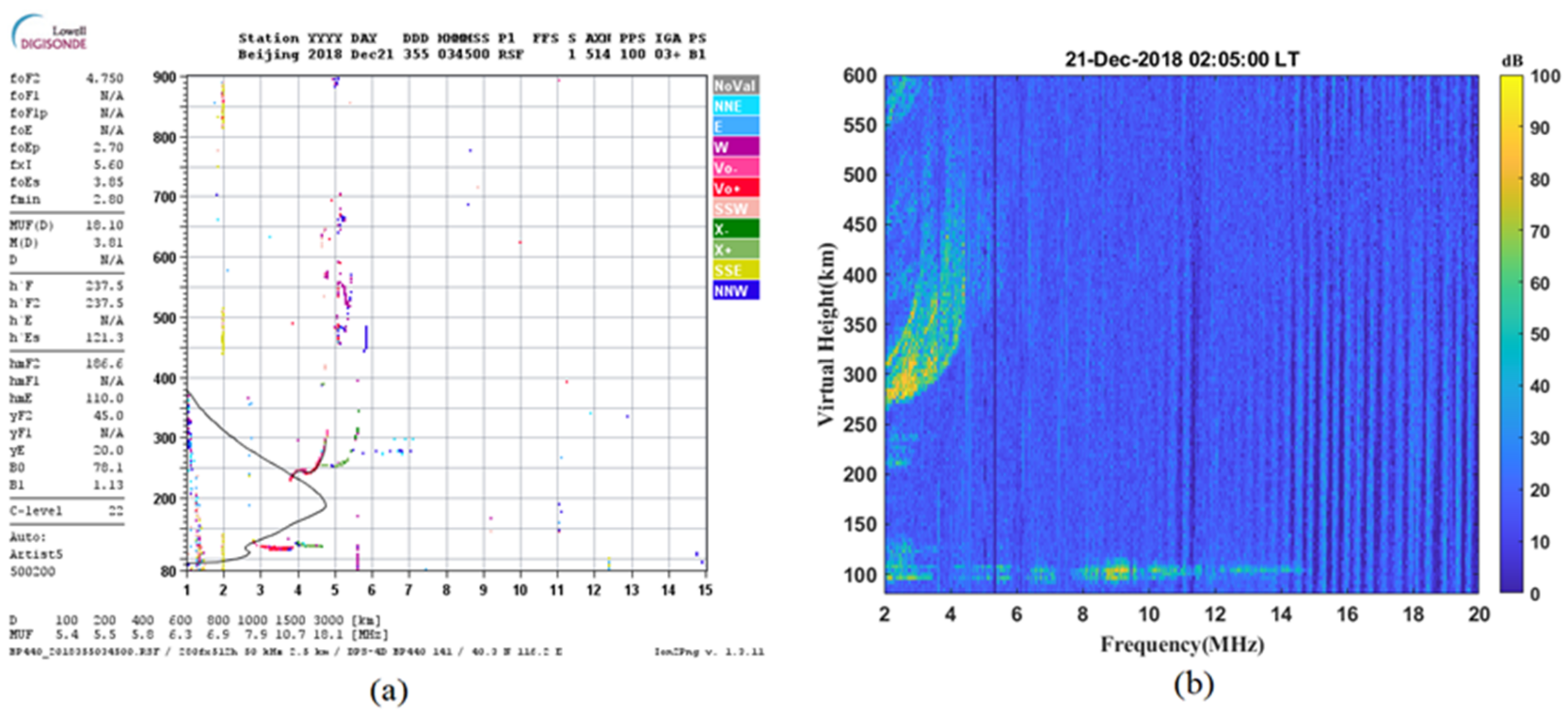
2. Data Sets and Methodology

The ionospheric parameters (the foEs and the h’Es) used in this study are from the two mid-latitude ionosondes, Beijing (40.25°N, 116.25°E) and Zhangye (39.21°N, 100.54°E) stations. Figure 1 shows the locations of these two stations. The digital ionosonde, named DPS-4D [22], is installed at Beijing station, which is sponsored by the Meridian Space Weather Monitoring Project. Another digital ionosonde at Zhangye, named Wuhan Ionospheric Sounder System (WISS) developed by the Ionospheric Laboratory of Wuhan University [23], has been installed at the edge of the Qinghai–Tibet Plateau.

In this study, only the Es layer with the foEs greater than 3 MHz is considered. The data resolution is 15 min and 5 min, respectively, at Beijing and Zhangye. For the convenience of statistics and comparisons, the data resolution used in this study is half hour for these two kinds of ionograms, then a data set was built with the size of 48 × 365 = 17,520. The period of the data is from January to December 2018.

Table 1. The distribution of data at Beijing and Zhangye.

Month	Number of Data Loss at Beijing	Data Loss Rate (%)	Number of Data Loss at Zhangye	Data Loss Rate (%)
1	31	2.083	32	2.151
2	0	0	508	37.798
3	1	0.067	170	11.425
4	13	0.902	435	30.208
5	310	20.833	26	1.747
6	12	0.833	0	0
7	7	0.470	0	0
8	9	0.605	6	0.403
9	12	0.833	0	0
10	27	1.815	0	0
11	1	0.069	0	0
12	5	0.336	2	0.134
Total	428	2.443	1179	6.729

shows the distribution of ionogram data at Beijing and Zhangye. The data loss means the number of missing data in each month. Figure 2 shows typical ionograms with Es layer recorded by these two ionosondes.

The parameters of the Es layer at two stations are scaled automatically first and then calibrated by manually. The ARTIST-5 is used for automatic scaling at Beijing station, while ionoScaler is used at Zhangye station. When the critical frequency of the Es layer is greater than the E layer, the echoes are identified as the Es layer.

There are some different characteristics between the ionosondes installed at Beijing and Zhangye. First, the DPS-4D was equipped with a double-channel receiver to separate the O-wave and X-wave. However, WISS has just a single-channel receiver, which cannot separate the O-wave and X-wave. Therefore, there is a slight discrepancy on the critical frequency of the Es layer. Second, two ionosondes also have different antennas, and the threshold amplitudes of the echoes are different in ionograms. These also affect the critical frequency and virtual base height of the Es layer. Fortunately, both DPS-4D and WISS have been installed at Wuhan station (The WISS installed at Zhangye station is the same type of WISS at Wuhan). Additionally, then the ionospheric parameters can be scaled from ionograms recorded by WISS that have been calibrated through the corresponding values from DPS-4D. Then, the system bias of the WISS can be estimated compared with DPS-4D. Finally, the estimated system bias was applied in the WISS at Zhangye station to overcome these issues mentioned above.

The occurrence probability of the Es layer was calculated by Equation (1).

$$P(LT,M)=\frac{n(LT,M)}{N(LT,M)}$$

(1)

where LT (Local Time) = 1~24, and M (Month) = 1~12. $n(LT,M)$ indicates the total number of the Es layer at the LT-th time of the M-th month and $N(LT,M)$ represents the total number of ionograms recorded by the ionosonde in the corresponding time.

3. Observations and Results

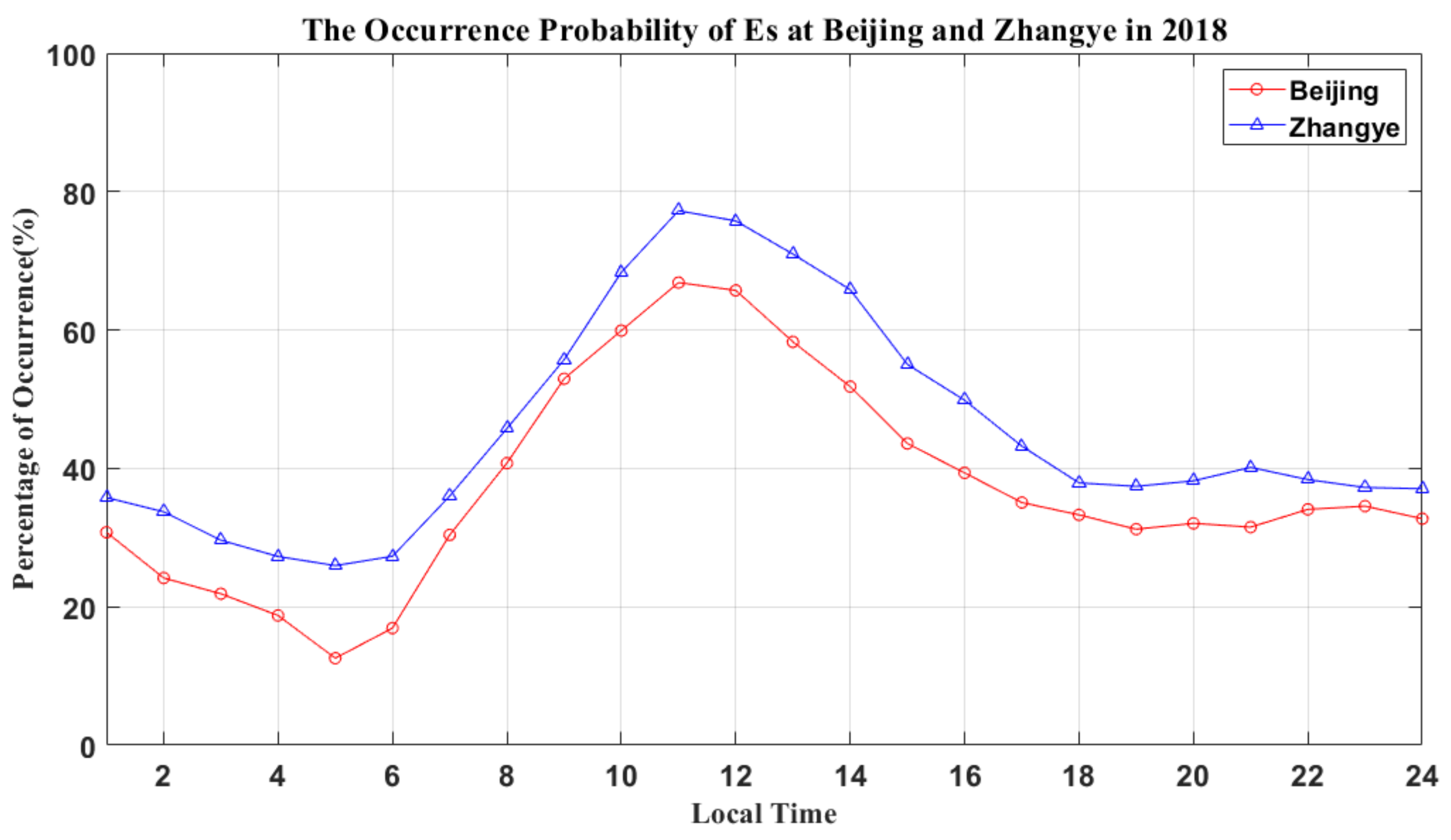
3.1. Comparison of Diurnal Changes in Es Layer

Figure 3 shows the average occurrence probability of the Es layer with local time at Beijing (red) and Zhangye (blue) stations during the year of 2018. The diurnal occurrence probability of the Es layer is in the range of 12.56–66.86% at Beijing and 25.95–77.24% at Zhangye. The occurrence probabilities at Beijing and Zhangye have almost the similar trend. The occurrence probabilities of the Es layer increase slowly after sunrise, the maximum values are at 11:00 LT, then slowly decrease and tend to be stable after 18:00 LT. They finally decrease slowly until sunrise. It can be seen from Figure 3 that the maximum occurrence probability of the Es layer is near the local noontime at Beijing and Zhangye. The probabilities of the Es layer are lower during the nighttime than daytime for these two stations. However, the probability of the Es layer is higher at Zhangye station than Beijing station at all local times. The rate difference between Beijing and Zhangye stations is about 2.69–14.10%.

Figure 4 shows the diurnal variations of foEs (Figure 4a) and their standard deviations (Figure 4b) recorded at Beijing (red) and Zhangye (blue) stations. In Figure 4, it can be found that the foEs at Beijing station is about 4.8–5.9 MHz in 2018. The variation in foEs at Zhangye fluctuates more compared with that at Beijing station. The foEs at Zhangye station is approximately 4.6–5.6 MHz. The maximum value of foEs is at 01:00 LT at Zhangye, and 21:00 LT at Beijing. In general, the difference in foEs between Beijing and Zhangye is slight and the trends of foEs at the two stations are similar.

Figure 5 shows the diurnal variations in h’Es (Figure 5a) and their standard deviations (Figure 5b) at Beijing and Zhangye. The h’Es at Beijing is about 106–119 km, but is about 105–115 km at Zhangye. It can be seen from Figure 5 that the h’Es at two stations begins to increase before sunrise (around 05:00 LT), and then reaches the maximum value at 07:00 LT. Subsequently, it began to slowly decrease in the early morning (after 07:00 LT) and increase again at 15:00 LT. Overall, the h’Es at Beijing is greater than Zhangye station except at 04:00 LT.

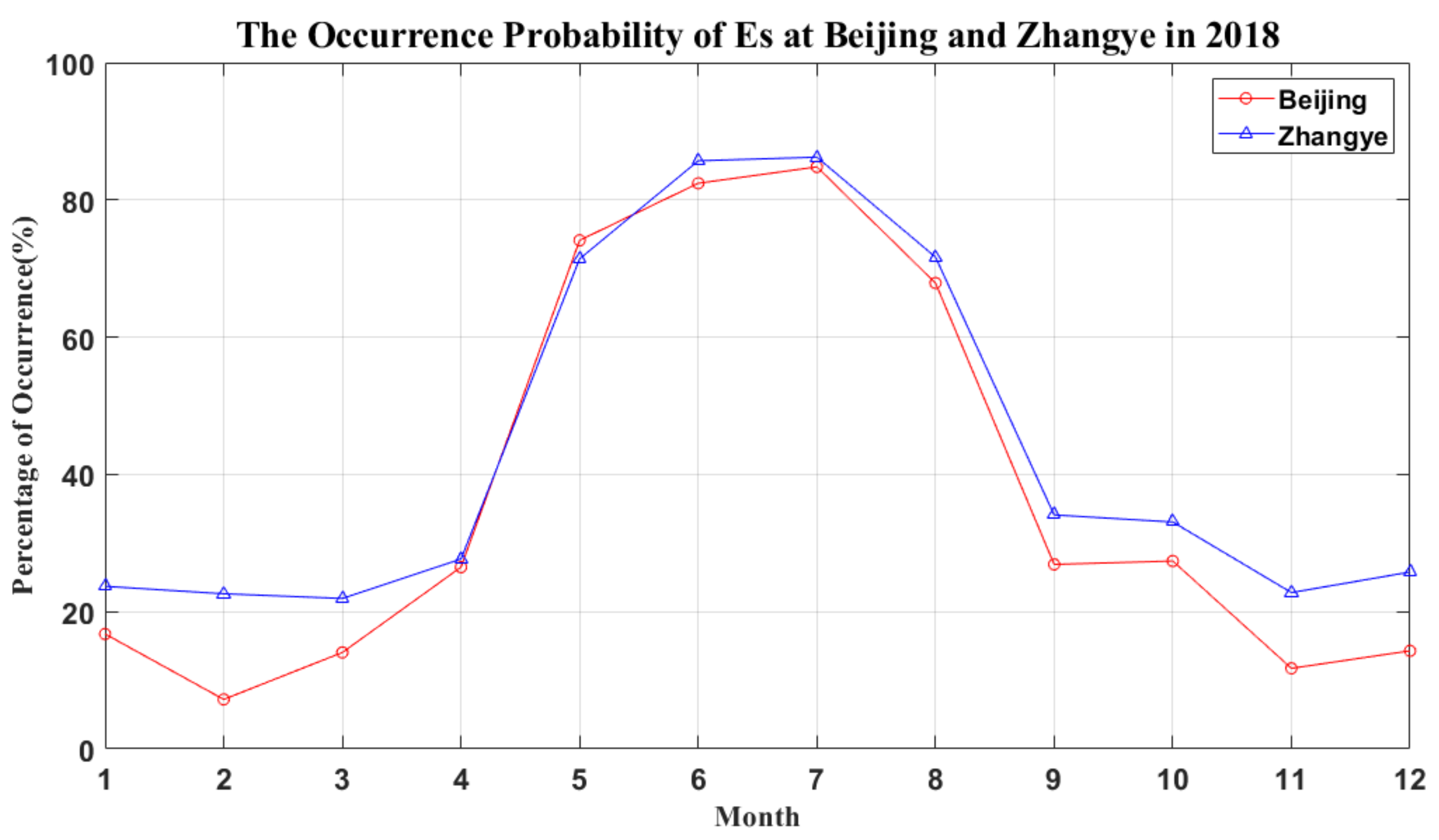
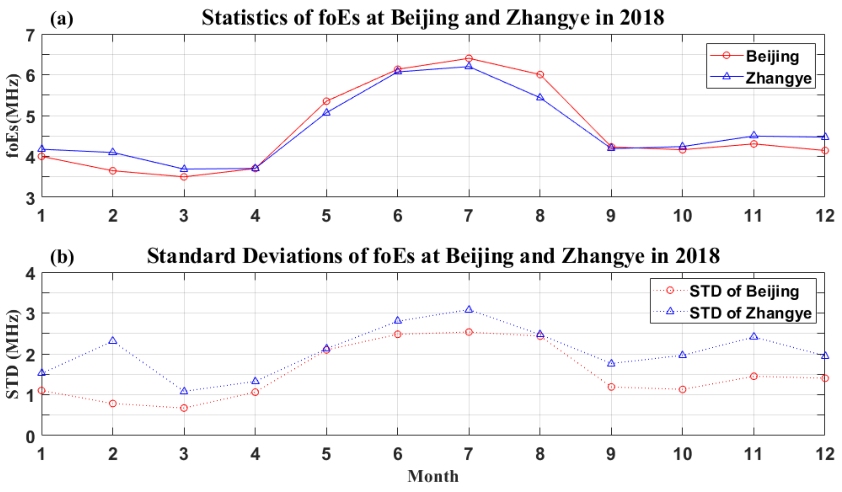
3.2. Comparison of Seasonal Changes in Es Layer

In order to study the seasonal variation in the Es layer, we divide the Es layer data into four seasons: spring (March–May), summer (June–August), autumn (September–November) and winter (December–February).

Figure 6, Figure 7 and Figure 8 show the seasonal variation in the Es layer at Beijing and Zhangye during the year of 2018. The red and blue lines in Figure 6, Figure 7 and Figure 8 represent, the average monthly values recorded at Beijing and Zhangye stations, respectively. It can be seen from Figure 6 that the maximum occurrence probability of the Es layer is in summer at Beijing and Zhangye stations. The monthly occurrence probability of the Es is in the range of 7.21–84.81% at Beijing, but is about 21.92–86.23% at Zhangye. In other months, the occurrence probability of the Es is much lower than the summer months. Generally, the occurrence probability is higher at Zhangye than that at Beijing, especially in early spring and winter season.

Figure 7 shows the average monthly critical frequency of the Es layer (foEs) (Figure 7a) and the standard deviation (Figure 7b). The characteristics of the intensity of the Es layer at Beijing and Zhangye are similar to previous studies. The intensity of the Es layer is greatest (about 6.40 MHz at Beijing and 6.20 MHz at Zhangye) in summer (July) but relatively low in other seasons. The difference in the monthly foEs average between Beijing and Zhangye is small.

Figure 8 shows the monthly variations in h’Es (Figure 8a) and their standard deviations (Figure 8b). The h’Es at Beijing station is 109.0 km–118.0 km and the maximum value of h’Es (118 km) occurred in April. The h’Es recorded at Zhangye is about 104 km–111 km. There is no significant disturbance in h’Es for the whole year. Generally, the h’Es is greater at Beijing than that at Zhangye.

Combining with the diurnal changes in the Es layer, it can be found that the difference in the average values of foEs and h’Es observed at Beijing and Zhangye is very small. This indicates that the morphological characteristics of the Es layer at these two stations are consistent, although the occurrence probabilities are different. That is to say, although the two stations have different sounding systems, the analysis of the Es layer shows that the data from these two stations are reliable.

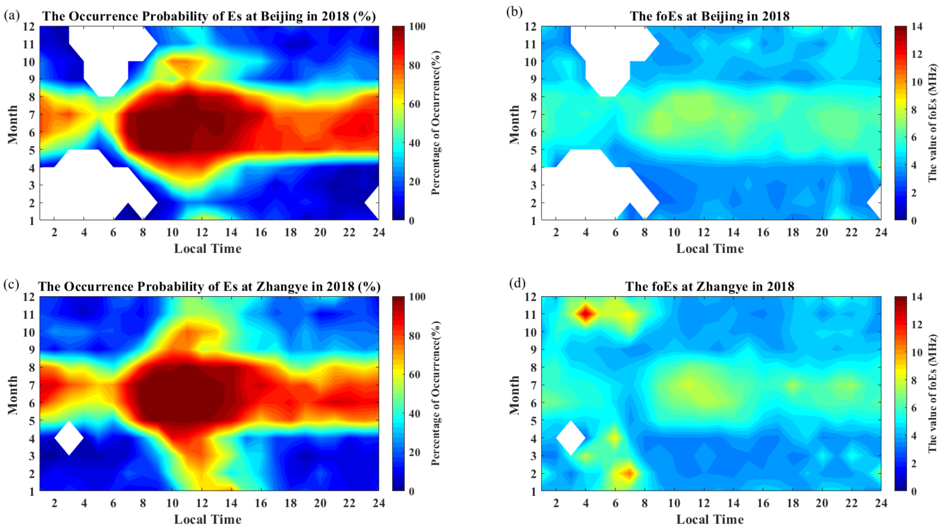
3.3. Es Layer Changes with Month and Local Time

To further study the characteristics of the Es layer at Beijing and Zhangye, the occurrence probability and foEs of the Es layer over local time and month was plotted, as shown in Figure 9. The white parts (the value is zero) represent the absence of an Es layer on ionograms at the Beijing and Zhangye stations.

In terms of the occurrence probability, the Es layer occurred frequently at Beijing and Zhangye stations in the summer season at all local times (please see Figure 9a,c). In terms of foEs, there is a large discrepancy in the intensity of the Es layer at Zhangye compared with observations at Beijing (please see Figure 9a,c). Figure 9b shows that the foEs at Beijing station is about 3.1–7.5 MHz, with a slight fluctuation throughout the year. The peak value is concentrated in the summer daytime. In winter and spring, foEs is small at night. Interestingly, the foEs is greater at Zhangye station in the equinox months and winter solstice than summer solstice during the nighttime (Please see Figure 9d). The foEs is between 3.1 MHz and 13.0 MHz at Zhangye. The maximum value mainly occurred at nighttime in winter and spring, and the second peak occurs during the daytime in summer.

Overall, during the daytime (07:00 LT–19:00 LT), the change characteristics of the foEs at Beijing and Zhangye are relatively consistent, the peak values occurred in the summer daytime, and the foEs in the rest of the seasons are very small. At nighttime (19:00 LT–07:00 LT), especially post-night to before sunrise, the value of foEs at Beijing is fewer, and Es does not even appear in the spring and winter. In contrast, the Es layer occurred frequently at Zhangye during the nighttime and sunrise and the foEs has a greater value. The foEs value is larger in winter and spring than that in summer at night. It shows that there is a significant anomaly in the occurrence probability and intensity of the Es layer in the nighttime during winter at Zhangye station.

Figure 10 shows the similar trend in daily mean values of foEs at Beijing and Zhangye stations. At the same time, it should be noted that the daily mean value of foEs at Zhangye has abnormally large values from the 312th day to the 360th day, and the abnormal phenomenon here can also be seen in Figure 9d.

Figure 11 shows the variation in foEs over days of the year and local time at two stations. The white parts represent the data missed at that moment, and the black parts represent the absence of an Es layer. The occurrence of the Es layer at Beijing and Zhangye is relatively consistent. It is worth noting that during the post-midnight period, the Es layer at Beijing can hardly be observed, while the Es at Zhangye occurred frequently, and the intensity of Es is very strong (the red box). It can also be seen in Figure 9d and Figure 10.

Statistical results show that observations of the Es layer at Beijing station are mostly consistent with previous results [19]. However, there are obvious anomalies in the nighttime (post-midnight) and winter to spring in the occurrence probability and intensity of the Es layer at Zhangye station. In the following section, we will discuss these anomalies in detail.

4. Discussion

Results show that the occurrence probability of the Es layer at Beijing and Zhangye has similar diurnal variations, with the maximum occurrence probability occurring at noontime. This can be explained by the classical wind shear theory, which believes that the local time characteristics of the occurrence of Es are controlled by the diurnal tidal wind and semidiurnal tidal wind [6,24]. The occurrence probability of the Es layer at Zhangye is larger than that at Beijing during all times. However, the diurnal variation in foEs/h’Es at Beijing is consistent with that at Zhangye (please see Figure 4 and Figure 5) which indicates that morphological characteristics of Es layer are similar at the two stations.

Pietrella and Bianchi [19] analyzed the 32-year ionospheric data at Rome (41.8°N, 12.5°E), the variations in the occurrence probability of the Es layer as a function of local time and month at Roman were plotted in Figure 1 of Pietrella and Bianchi [19]. In this study, Figure 9a,c is similar with Figure 1 in Pietrella and Bianchi [19], and the occurrence probability of the Es layer with foEs greater than 3 MHz was considered. In addition, these three stations are also located at middle latitudes. Therefore, we can compare the diurnal variation in the three stations. The maxima of the occurrence probability are all at noontime in the summer months at the three stations. Note that the occurrence probabilities in 07:00 LT–18:00 LT in May, June, July and August are more than 80% at all stations. Interestingly, small bulges exist at 17:00 LT in October at both Beijing and Rome, while the bulge becomes not obvious due to the high occurrence probability of Es in winter at Zhangye. Overall, the occurrence probabilities of the Es layer in the three stations are very similar, but the occurrence rate is slightly higher at Zhangye.

In terms of seasonal variations, as mentioned above, the maximum occurrence probability of the Es layer is in summer at both Beijing and Zhangye. The seasonal characteristics of the Es layer at Beijing and Zhangye are similar with those at Rome [19]. In summer, the occurrence probabilities of the Es layer are more than 80% during the daytime at the three stations. However, in spring and winter, the Es layers mainly appear at noontime at the three stations, which with the occurrence probabilities are more than 40%. Note that the Es layers during sunset and midnight in winter are slightly active at all stations, with the occurrence probabilities being around 20%.

This is consistent with the general belief that the occurrence of the Es layer has an obvious seasonal characteristic [7]. There are two reasons for this seasonal characteristic. One is that the maximum value of sporadic meteor deposition is in summer [16]. The other is the direction of the shear of vertical ion velocity in the E region. Taking Na⁺ for an example [25], the vertical shear of vertical ion velocity is negative and positive, respectively, above and below 100 km in summer. It is a favorable condition for forming the ion convergence layer. However, in winter, the shear of vertical ion velocity is mostly negative.

Nevertheless, unlike the conventional characteristics related to the summer maximum and winter minimum at Beijing, the occurrence probability of the Es layer still maintains a large value at Zhangye in winter and spring (more than 20%). There is a relatively large discrepancy in the occurrence probability between the two stations in winter and spring. It shows that the occurrence probability of the Es layer at Zhangye has obvious seasonal anomalies. This anomaly can also be seen in the seasonal variation in foEs (from Figure 9b,d). The seasonal variation trend of foEs (which is known for many years, the maxima in summer) at Beijing is similar to that at Athens (38.0°N, 23.44°E), San Vito (40.60°N, 9.54°E) and Boulder (40.0°N, 105°W) [16]. The summer maxima of daily mean values of foEs are about 5.0 MHz, 6.7 MHz, 6.4 MHz and 8.4 MHz, at Athens, San Vito, Boulder and Beijing, respectively. While the winter minima of daily mean values of foEs are about 2.6 MHz, 2.2 MHz, 1.5 MHz and 3.0 MHz, at the four stations, respectively. The mean values of foEs at Beijing are greater than those at the other three stations. That is because only the Es layer with the foEs greater than 3 MHz is considered in our study, which causes the greater daily mean values of foEs at Beijing. However, the maximum of foEs at Zhangye appears in winter and early spring.

Combining the results of Figure 10 and Figure 11, the occurrence probability and intensity of the Es layer at Zhangye station are abnormal from winter to spring and at night. Especially in the period of post-midnight in winter, the abnormal phenomenon at Zhangye is particularly obvious.

In order to reveal the reason for the anomalies of the Es layer at Zhangye, we need to have a clearer understanding of the formation of the Es layer. The classical wind shear theory shows that vertical ion convergence driven by vertical shears in the horizontal neutral wind can form the Es layer in the dynamo region of the ionosphere [7]. Chu et al. [26] simulated the global seasonal distribution of global Fe⁺ ion flux and found that it has a good correlation with the global distribution of the Es. According to the model simulation by Chu et al. [26], the distribution and existence of Fe⁺ ions at Beijing and Zhangye are basically at the same level. Note that the different metal ions in the Es layer have almost similar behavior although their vertical ion velocities are different due to different atomic mass [25,27]. Therefore, the density levels and behaviors of other ions at Beijing and Zhangye are similar. It can be found that the metal ion flux cannot explain the two abnormal phenomena mentioned above, the occurrence probability and intensity of the Es layer at Zhangye at night and winter to spring.

Yu et al. [20] studied the long-term climatology of the Es layer by using COSMIC GPS radio occultation measurement data from December 2006 to January 2014. They concluded that in addition to vertical wind shear, the vertical motion of gravity waves, magnetic field effects, the flux injected by meteors and the chemical process of metal ions may all play a role in the geographic and seasonal changes in the intensity of the Es layer. In terms of magnetic field effects, the geomagnetic inclination angles of Beijing and Zhangye are close (59.4 and 59.5 degree), so there is no significant difference in the horizontal component of geomagnetism. In addition, the meteoric influx, accounting for the seasonal dependence marked by the summer maximum [16], also cannot explain the phenomena at Zhangye. Therefore, it is reasonable to think that the gravity waves might be a factor in forming this abnormal anomaly.

It is noted that the sporadic metal layers are frequently accompanied with the occurrence of the Es layer [18,28]. Therefore, the statistics of the sporadic metal layers can also partly reveal the character of the Es layer. Cai et al. [25] numerically simulated the Na⁺ by a statistical study based on seven-year Na lidar observations at Logan, UT (41.7°N, 112°W) and twelve-year Na lidar observations at Arecibo Observatory, PR (18.3°N, 67°W). The statistical results show that the sporadic sodium layer has higher occurrence in winter at PR than UT, and then they calculated and compare the PED (potential energy density, which can partly reflect gravity wave activity) between PR and UT. They found that the gravity wave activity at PR in winter is more active than that in UT, which is a possible reason to explain the statistical results.

Coincidentally, we know that Zhangye is located at the edge of the Qinghai–Tibet Plateau, where there is a more active region in gravity waves. The gravity wave activity at Beijing is relatively weaker. Therefore, the anomalies of the Es layer at Zhangye station might be caused by gravity waves from the lower atmosphere. In other words, the gravity waves might cause the neutral wind shear to be more active at Zhangye station, and then the convergence of metallic ion flux should be larger at Zhangye than Beijing.

Many studies [29,30,31,32] suggest that gravity waves play a critical role in the formation of the Es layer. Didebulidz et al. [33] proposed the mechanism by which gravity waves affect the generation of the Es layer. Atmospheric gravity waves with vertical wavelengths smaller than the width of the lower thermal layer will cause the appearance of vertical drift velocity nodes of heavy metal ions (Fe⁺) (regions where the vertical drift velocity of ions caused by these waves is zero), when the divergence of the ion vertical drift velocity at its node is the smallest negative value, these charged particles can accumulate into an Es-type thin layer, thereby forming an Es layer with a multilayer structure.

The nighttime anomaly (post-midnight in winter) in the occurrence probability and intensity of the Es layer at Zhangye may be caused by the diurnal variation in gravity waves. Yao et al. [34] used AIRS (Atmospheric Infrared Sounder) observations in the summer of 2007 to analyze deep convection and gravity waves in East Asia and showed that the frequency and intensity of disturbances in the stratosphere at night were significantly greater than those at nighttime. The research by Qian et al. [35] also confirms this point. Through the diurnal variation analysis of gravity waves in the Qinghai–Tibet Plateau in the summer of 2015, it is found that the power spectrum of gravity waves is weakest at noon and strongest at midnight. The energy contributed by mesoscale atmospheric processes is strongest at midnight (18 UTC) and the weakest power curve is at noon (06 UTC). It can be found that the diurnal variation characteristics of gravity waves are consistent with that of the Es layer at Zhangye (from Figure 9d and Figure 11d). Then, we might conclude that the diurnal variation in the gravity wave activity might be the cause of the nighttime anomaly of foEs, that is, gravity wave activity plays an important role in the modulation of the diurnal variation in the intensity of the Es layer.

Regarding seasonal variations in the Es layer, we found that the seasonal characteristics of atmospheric gravity waves in the Qinghai–Tibet Plateau are also consistent with the characteristics of the Es layer at Zhangye station. The plateau atmospheric gravity waves are most active in winter and spring and are calmer in summer and autumn [36,37]. The maximum intensity of the Es layer at Zhangye and the maximum discrepancy in the occurrence probability of the Es layer between these two stations appeared in winter and early spring (from Figure 9). This anomaly might be related to the seasonal characteristics of the gravity waves. The strong gravity wave activity might promote the concentration of metal ions in the ionosphere at Zhangye station, thereby increasing the occurrence probability of Es in winter and spring. The strength of gravity wave activity also affects the intensity of the Es layer at Zhangye station, which caused the occurrence of the winter enhancement. On the contrary, the atmospheric density disturbance caused by the gravity wave in the Beijing area has the activity rule that is larger in summer than that in winter [38]. As a result, the seasonal characteristics of the gravity wave at Beijing are consistent with the seasonal characteristics of the Es layer. This might explain why the anomalies in the characteristics of the Es layer did not occur at Beijing. Combined with the diurnal characteristics of the gravity waves, it suggests that the abnormal characteristics of the Es layer at Zhangye station might be due to gravity waves. Generally, the amplitude of gravity waves in the MLT region is small scale [39]. However, the spatial resolution of observations by SABER [40,41] is too low for this comparative study between Beijing and Zhangye stations. Therefore, it is difficult to distinguish the characteristics of the gravity waves at these two stations.

In terms of the base virtual height (h’Es), the statistical results are similar with the features observed by the research of Wang et al. [42] using the 11-year observation data of ionosonde in the Qingdao area (36.24°N, 120.42°E). These results show that the seasonal variation and diurnal variation in the virtual height have a dual-peak structure, with April and September as the primary and secondary peaks for the whole year, while 07:00 LT and 17:00 LT as the peaks in the diurnal variation. Our results suggest that 07:00 LT and 18:00 LT as the peaks in terms of diurnal variation, which is almost similar to Wang et al. [42]. In addition, Figure 5 and Figure 8 show that the difference in h’Es parameters between Beijing and Zhangye is relatively small and meets the height range of the Es layer; therefore, we did not discuss this in detail in this study.

5. Conclusions

This study used ionosonde observations of the Es layer between the plateau and plain regions in China to conduct the statistical characteristics of the Es layer in the middle region. The key results from the present study are listed below.

(1)

The diurnal characteristics of the occurrence probability in the Es layer are similar at the Beijing and Zhangye stations, with a maximum value at noontime. However, during the post-midnight period in winter, the Es layer occurred more frequently at Zhangye station than at Beijing. In terms of the intensity of the Es layer (foEs), there is a large discrepancy between the two stations. The maximum mean value of foEs occurred at nighttime at Zhangye (from Figure 9d and Figure 10), inconsistent with the observations from Beijing station. There is an obvious night anomaly in the intensity of the Es layer at Zhangye.

(2)

The seasonal variations in the occurrence probability of the Es layer at Beijing and Zhangye are similar (the maximum summer). The occurrence of the Es layer at Zhangye is higher than Beijing throughout the year (except May). The discrepancy in the occurrence of the Es layer between the two stations is larger in winter and early spring and smaller in summer. In terms of the monthly mean of foEs, the maxima are in summer at Zhangye and Beijing stations. However, in winter and early spring, the mean values of foEs at Zhangye station are slightly larger than that at Beijing station, but the opposite in other seasons. In terms of the daily mean value of foEs, the maximum daily mean value occurred in winter at Zhangye station. In terms of the occurrence probability and intensity of Es, there is pronounced anomaly (post-midnight) at Zhangye compared with the observations from Beijing station.

(3)

The anomalies of the Es layer at night and in winter to spring at Zhangye station might be attributed to the gravity wave activity in the Qinghai–Tibet Plateau. The power spectrum of gravity waves in the Qinghai–Tibet Plateau is weakest at noontime and strongest at midnight. The diurnal variations are consistent with the night anomaly of the Es layer at Zhangye station. The strength of the gravity waves is stronger in winter and spring than in summer and autumn. We found that the seasonal characteristics of the gravity waves are also consistent with the winter anomaly of the Es layer at Zhangye station.

References

1. Houminer, Z.; Russel, C.J.; Dyson, P.L.; Bennet, J.A. Study of sporadic-E clouds by backscatter radar. Ann. Geophys. 1996, 14, 1060–1065. [Google Scholar] [CrossRef]
2. Raizada, S.; Tepley, C.A.; Zhou, Q.; Sarkhel, S.; Mathews, J.D.; Aponte, N.A.; Cabassa, E. Dependence of mesospheric Na and Fe distributions on electron density at Arecibo. Earth Planets Space 2015, 67, 146. [Google Scholar] [CrossRef] [Green Version]
3. Wei, L.; Jiang, C.; Hu, Y.; Aa, E.; Huang, W.; Liu, J.; Yang, G.; Zhao, Z. Ionosonde Observations of Spread F and Spread Es at Low and Middle Latitudes during the Recovery Phase of the 7–9 September 2017 Geomagnetic Storm. Remote Sens. 2021, 13, 1010. [Google Scholar] [CrossRef]
4. Whitehead, J.D. The formation of the sporadic E layer in the temperate zones. J. Atmos. Sol. Terr. Phys. 1961, 20, 49–58. [Google Scholar] [CrossRef]
5. Axford, W.I. The formation and vertical movement of dense ionized layers in the ionosphere. J. Geophys. Res. 1963, 68, 769–779. [Google Scholar] [CrossRef]
6. Whitehead, J.D. Production and prediction of sporadic-E. J. Rev. Geophys. 1970, 8, 65–144. [Google Scholar] [CrossRef]
7. Whitehead, J.D. Recent work on mid-latitude and equatorial sporadic-E. J. Atmos. Terr. Phys. 1989, 51, 401–424. [Google Scholar] [CrossRef]
8. Mathews, J.D. Sporadic E: Current views and recent progress. J. Atmos. Sol. Terr. Phys. 1998, 60, 413–435. [Google Scholar] [CrossRef]
9. Haldoupis, C.; Pancheva, D. Planetary waves and midlatitude sporadic E layers: Strong experimental evidence for a close relationship. J. Geophys. Res. 2002, 107, A6. [Google Scholar] [CrossRef]
10. Pancheva, D.; Haldoupis, C.; Meek, C.E.; Manson, A.H.; Mitchell, N.J. Evidence of a role for modulated atmospheric tides in the dependence of sporadic E layers on planetary waves. J. Geophys. Res. 2003, 108, 1176. [Google Scholar] [CrossRef]
11. Arras, C.; Jacobi, C.; Wickert, J. Semidiurnal tidal signature in sporadic E occurrence rates derived from GPS radio occultation measurements at higher midlatitudes. Ann. Geophys. 2009, 27, 2555–2563. [Google Scholar] [CrossRef] [Green Version]
12. Zhou, C.; Tang, Q.; Song, X.X.; Qing, H.Y.; Liu, Y.; Wang, X.; Gu, X.D.; Ni, B.B.; Zhao, Z.Y. A statistical analysis of sporadic E layer occurrence in the midlatitude China region. J. Geophys. Res. 2017, 122, 3617–3631. [Google Scholar] [CrossRef]
13. Haldoupis, C.; Pancheva, D.D. Terdiurnal tidelike variability in sporadic E layers. J. Geophys. Res. 2006, 11, A07303. [Google Scholar] [CrossRef]
14. Haldoupis, C.; Meek, C.; Christakis, N.; Pancheva, D.; Bourdillon, A. Lonogram height-time-intensity observations of descending sporadic E layers at mid-latitude. J. Atmos. Sol. Terr. Phys. 2006, 68, 539–557. [Google Scholar] [CrossRef] [Green Version]
15. Arras, C.; Wickert, J.; Beyerle, G.; Heise, S.; Schmidt, T.; Jacobi, C. A global climatology of ionospheric irregularities derived from GPS radio occultation. Geophys. Res. Lett. 2008, 35, 14. [Google Scholar] [CrossRef]
16. Haldoupis, C.; Pancheva, D.; Singer, W.; Meek, C.; MacDougall, J. An explanation for the seasonal dependence of midlatitude sporadic E layers. J. Geophys. Res. Space Phys. 2007, 112, A06315. [Google Scholar] [CrossRef]
17. Dou, X.K.; Qiu, S.C.; Xue, X.H.; Chen, T.D.; Ning, B.Q. Sporadic and thermospheric enhanced sodium layers observed by a lidar chain over China. J. Geophys. Res. Space Phys. 2013, 118, 6627–6643. [Google Scholar] [CrossRef]
18. Williams, B.P.; Berkey, F.T.; Sherman, J.; She, C.Y. Coincident extremely large sporadic sodium and sporadic E layers observed in the lower thermosphere over Colorado and Utah. Ann. Geophys. 2007, 25, 3–8. [Google Scholar] [CrossRef] [Green Version]
19. Pietrella, M.; Bianchi, C. Occurrence of sporadic-E layer over the ionospheric station of Rome: Analysis of data for thirty-two years. Adv. Space Res. 2009, 44, 72–81. [Google Scholar] [CrossRef]
20. Yu, B.; Xue, X.; Yue, X.; Yang, C.; Yu, C.; Dou, X.; Ning, B.; Hu, L. The global climatology of the intensity of the ionospheric sporadic E layer. Atmos. Chem. Phys. 2019, 19, 4139–4151. [Google Scholar] [CrossRef] [Green Version]
21. Pietrella, M.; Pezzopane, M.; Bianchi, C. A comparative sporadic-E layer study between two mid-latitude ionospheric stations. Adv. Space Res. 2014, 54, 150–160. [Google Scholar] [CrossRef]
22. Reinisch, B.W.; Galkin, I.A.; Khmyrov, G.M.; Kozlov, A.V.; Lisysyan, I.A.; Bibl, K.; Cheney, G.; Kitrosser, D.F.; Stelmash, S.; Roche, K.; et al. Advancing Digisonde technology: The DPS-4D, in Radio Sounding and Plasma Physics. AIP Conf. Proc. 2008, 974, 127–143. [Google Scholar] [CrossRef]
23. Shi, S.; Yang, G.; Jiang, C.; Zhang, Y.; Zhao, Z. Wuhan Ionospheric Oblique Backscattering Sounding System and Its Applications—A Review. Sensors 2016, 17, 1430. [Google Scholar] [CrossRef] [Green Version]
24. Matsushita, S.; Reddy, C.A. A study of blanketing sporadic E at middle latitudes. J. Geophys. Res. 1967, 72, 2903–2916. [Google Scholar] [CrossRef]
25. Cai, X.; Yuan, T.; Eccles, J.V.; Raizada, S. Investigation on the distinct nocturnal secondary sodium layer behavior above 95 km in winter and summer over Logan, UT (41.7°N, 112°W) and Arecibo Observatory, PR (18.3°N, 67°W). J. Geophys. Res. Space Phys. 2019, 124, 9610–9625. [Google Scholar] [CrossRef]
26. Chu, Y.; Wang, C.; Wu, K.; Chen, K.; Tzeng, K.J.; Su, C.; Feng, W.; Plane, J.M.C. Morphology of sporadic E layer retrieved from COSMIC GPS radio occultation measurements: Wind shear theory examination. J. Geophys. Res. Space 2014, 119, 2117–2136. [Google Scholar] [CrossRef]
27. Plane, J.M.C.; Feng, W.; Dawkins, E.C.M. The Mesosphere and Metals. Chem. Chang. Chem. Rev. 2015, 115, 4497–4541. [Google Scholar] [CrossRef] [PubMed]
28. Dou, X.-K.; Xue, X.-H.; Li, T.; Chen, T.-D.; Chen, C.; Qiu, S.-C. Possible relations between meteors, enhanced electron density layers, and sporadic sodium layers. J. Geophys. Res. Space Phys. 2010, 115, A6. [Google Scholar] [CrossRef] [Green Version]
29. MacDougall, J.W. 110 km neutral zonal wind patterns. Planet. Space Sci. 1974, 22, 545–558. [Google Scholar] [CrossRef]
30. Wilkinson, P.J.; Szuszczewicz, E.P.; Roble, R.G. Measurements and modelling of intermediate, descending, and sporadic layers in the lower ionosphere: Results and implications for global-scale ionosphericthermospheric studies. Geophys. Res. Lett. 1992, 19, 95–98. [Google Scholar] [CrossRef]
31. Haldoupis, C. Midlatitude sporadic E. A typical paradigm of atmosphereionosphere coupling. Space Sci. Rev. 2012, 168, 441–461. [Google Scholar] [CrossRef]
32. Liu, Y.; Zhou, C.; Xu, T.; Tang, Q.; Deng, Z.X.; Chen, G.Y.; Wang, Z.K. Review of ionospheric irregularities and ionospheric electrodynamic coupling in the middle latitude region. Earth Planet. Phys. 2021, 5, 462–482. [Google Scholar] [CrossRef]
33. Didebulidze, G.G.; Dalakishvili, G.; Todua, M. Formation of Multilayered Sporadic E under an Influence of Atmospheric Gravity Waves (AGWs). Atmosphere 2020, 11, 653. [Google Scholar] [CrossRef]
34. Yao, Z.-G.; Zhao, Z.-L.; Han, Z.-G. Stratospheric gravity waves during summer over East Asia derived from AIRS observations. Chin. J. Geophys. 2015, 58, 1121–1134. [Google Scholar] [CrossRef]
35. Qian, T.; Zhang, F.; Wei, J.; He, J.; Lu, Y. Diurnal Characteristics of Gravity Waves over the Tibetan Plateau in 2015 Summer Using 10-km Downscaled Simulations from WRF-EnKF Regional Reanalysis. Atmosphere 2020, 11, 631. [Google Scholar] [CrossRef]
36. Zeng, X.; Xue, X.; Dou, X.; Liang, C.; Jia, M. COSMIC GPS observations of topographic gravity waves in the stratosphere around the Tibetan Plateau. Sci. China Earth Sci. 2016, 60, 188–197. [Google Scholar] [CrossRef]
37. Xu, X.H.; Guo, J.C.; Luo, J. Analysis of the active characteristics of stratosphere gravity waves over the Qinghai-Tibetan Plateau using COSMIC radio occultation data. Chin. J. Geophys. 2016, 59, 1199–1210. (In Chinese) [Google Scholar] [CrossRef]
38. Zou, X.; Yang, G.; Wang, J.; Gong, S.; Cheng, X.; Jiao, J.; Yue, C.; Fu, H.; Wang, Z.; Yang, S.; et al. Gravity wave parameters and their seasonal variations derived from Na lidar observations at Beijing. Chin. J. Space Sci. 2015, 35, 453–460. (In Chinese) [Google Scholar] [CrossRef]
39. Smith, A.K. Global dynamics of the MLT. Surv. Geophys. 2012, 33, 1177–1230. [Google Scholar] [CrossRef] [Green Version]
40. Liu, X.; Yue, J.; Xu, J.; Garcia, R.R.; Russell, J.M.; Mlynczak, M.; Wu, D.L.; Nakamura, T. Variations of global gravity waves derived from 14 years of SABER temperature observations. J. Geophys. Res. Atmos. 2017, 122, 6231–6249. [Google Scholar] [CrossRef]
41. Preusse, P.; Eckermann, S.D.; Ern, M.; Oberheide, J.; Picard, R.H.; Roble, R.G.; Riese, M.; Russell, J.M., III; Mlynczak, M.G. Global ray tracing simulations of the SABER gravity wave climatology. J. Geophys. Res. Atmos. 2009, 114, D8. [Google Scholar] [CrossRef]
42. Xiaobin, W.; Zhengzheng, M.A.; Yabin, Z. Statistical analysis on characteristics of Es in Qingdao region. Chin. J. Radio Sci. 2014, 29, 969–972+993. (In Chinese) [Google Scholar] [CrossRef]
Figure 1. The locations of Beijing (40.25°N, 116.25°E) and Zhangye (39.21°N, 100.54°E).
Remotesensing 14 02871 g001
Figure 2. Typical ionograms of the Es layer at Beijing (a) and Zhangye (b) stations on 21 December 2018.
Remotesensing 14 02871 g002
Figure 3. Diurnal variations in the occurrence probability of the Es layer at Beijing and Zhangye stations.
Remotesensing 14 02871 g003
Figure 4. Diurnal variations in mean values (a) and standard deviations (b) of foEs at Beijing and Zhangye stations.
Remotesensing 14 02871 g004
Figure 5. Diurnal variations in mean values (a) and standard deviations (b) of h’Es at Beijing and Zhangye stations.
Remotesensing 14 02871 g005
Figure 6. Seasonal changes in the occurrence probability of the Es layer at Beijing and Zhangye stations.
Remotesensing 14 02871 g006
Figure 7. Seasonal changes in mean values (a) and standard deviations (b) of foEs in the Es layer at Beijing and Zhangye stations.
Remotesensing 14 02871 g007
Figure 8. Seasonal changes in mean values (a) and standard deviations (b) of h’Es at Beijing and Zhangye stations.
Remotesensing 14 02871 g008
Figure 9. Variations in the occurrence probability and foEs of the Es layer as a function of local time and month at Beijing (a,b) and Zhangye (c,d) stations.
Remotesensing 14 02871 g009
Figure 10. Comparison of the annual variation in daily mean of foEs measured by the Beijing ionosonde (red) and Zhangye ionosonde (grey) in 2018.
Remotesensing 14 02871 g010
Figure 11. Variations in foEs as a function of day of the year and local time at Beijing (a) and Zhangye (b) stations.
Remotesensing 14 02871 g011