
An Improved Spatially Variant MOCO Approach Based on an MDA for High-Resolution UAV SAR Imaging with Large Measurement Errors

Abstract
:
1. Introduction
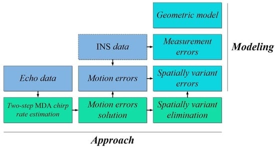
2. Modeling
2.1. Geometric Model
2.2. Spatially Variant Errors Analyses
2.3. Measurement Errors Analyses
- (1)
- Gyroscope north bias: The yaw angle of the platform is measured by a gyroscope, which is an important component of an INS. However, this bias affects the measured heading and further changes the Doppler centroid. Thus, the position is shifted.
- (2)
- Data rate: In practice, motion data is sampled from INS measurements and saved by recorder. However, it is difficult to synchronize the chirp frame with motion data accurately because the data rate of an INS is much smaller than pulse repetition frequency (PRF) which indicates that the measurement errors are inevitable, and the Doppler chirp rate is changed and thus de-focused.
- (3)
- Random noise: Random noise exists in all kinds of electronic devices. INS noise introduces the extra high-frequency phase errors during MOCO and raises the grating lobe.
3. Approach
3.1. Two-Step MDA Chirp Rate Estimation
3.1.1. Sub-Aperture Processing
3.1.2. Map-Drift Chirp Rate Estimation
3.1.3. Coarse and Precise Processing
3.2. Motion Errors Solution
3.2.1. NPEs Equations Construction
3.2.2. RANSAC Solution
3.3. Spatially Variant Estimation
3.3.1. Decoupling Processing Based on 2D Mapping
3.3.2. CZT Correction
4. Experiment
4.1. Simulation Results
4.2. Real Data Experiment Results
5. Conclusions
Author Contributions
Funding
Conflicts of Interest
References
- Carrara, W.G.; Goodman, R.S. Spotlight Synthetic Aperture Radar: Signal Processing Algorithms; Artech House: Boston, MA, USA, 1995; pp. 245–254. [Google Scholar]
- Cumming, I.G.; Wong, F.H. Digital Processing of Synthetic Aperture Radar Data: Algorithm and Implementation; Artech House: Boston, MA, USA, 2005; pp. 567–586. [Google Scholar]
- Curlander, J.C.; McDonough, R.N. Synthetic Aperture Radar: Systems and Signal Processing; Wiley: New York, NY, USA, 1991; pp. 178–212. [Google Scholar]
- Li, Z.; Ye, H.; Liu, Z.; Sun, Z.; An, H.; Wu, J.; Yang, J. Bistatic SAR clutter-ridge matched STAP method for non-stationary clutter suppression. IEEE Trans. Geosci. Remote Sens. 2022, 60, 1–14. [Google Scholar]
- Li, Z.; Huang, C.; Sun, Z.; An, H.; Wu, J.; Yang, J. BeiDou-Based passive multistatic radar maritime moving target detection technique via space time hybrid integration processing. IEEE Trans. Geosci. Remote Sens. 2022, 60, 1–13. [Google Scholar] [CrossRef]
- Kim, S.; Jeon, S.Y.; Kim, J.; Lee, U.M.; Shin, S.; Choi, Y.; Ka, M.H. Multichannel W-Band SAR system on a multirotor UAV platform with real-time data transmission capabilities. IEEE Access 2020, 8, 144413–144431. [Google Scholar] [CrossRef]
- Chen, K.S. Principles of Synthetic Aperture Radar Imaging: A System Simulation Approach; CRC Press: Boca Raton, FL, USA, 2016; pp. 111–129. [Google Scholar]
- Xing, M.; Jiang, X.; Wu, R.; Zhou, F.; Bao, Z. Motion compensation for UAV SAR based on raw radar data. IEEE Trans. Geosci. Remote Sens. 2009, 47, 2870–2883. [Google Scholar] [CrossRef]
- Tang, S.; Zhang, L.; Guo, P.; Liu, G.; Sun, G. Acceleration model analyses and imaging algorithm for highly squinted airborne spotlight-mode SAR with maneuvers. IEEE J. Sel. Top. Appl. Earth Obs. Remote Sens. 2015, 8, 1120–1131. [Google Scholar] [CrossRef]
- Xu, W.; Wang, B.; Xiang, M.; Wang, S.; Jianfeng, Y. A novel motion compensation approach based on symmetric triangle wave interferometry for UAV SAR imagery. IEEE Access 2020, 8, 104996–105007. [Google Scholar] [CrossRef]
- Chen, J.; Liang, B.; Zhang, J.; Yang, D.G.; Deng, Y.; Xing, M. Efficiency and robustness improvement of airborne SAR motion compensation with high resolution and wide swath. IEEE Trans. Geosci. Remote Sens. 2022, 19, 1–5. [Google Scholar] [CrossRef]
- Bie, B.; Xing, M.; Xia, X.; Sun, G.; Liang, Y.; Jing, G.; Wei, T.; Yang, Y. A Frequency Domain Backprojection Algorithm based on local cartesian coordinate and subregion range migration correction for high-squint SAR mounted on maneuvering platforms. IEEE Trans. Geosci. Remote Sens. 2018, 56, 7086–7101. [Google Scholar] [CrossRef]
- Luo, Y.; Zhao, F.; Li, N.; Zhang, H. A modified cartesian factorized back-projection algorithm for highly squint spotlight synthetic aperture radar imaging. IEEE Geosci. Remote Sens. Lett. 2019, 16, 902–906. [Google Scholar] [CrossRef]
- Wahl, D.E.; Eichel, D.C.; Ghiglia, C.V.; Jakowatz, J.R. Phase gradient autofocus–a robust tool for high resolution SAR phase correction. IEEE Trans. Aerosp. Electron. Syst. 1994, 30, 827–835. [Google Scholar] [CrossRef] [Green Version]
- Miao, Y.; Wu, J.; Yang, J. Azimuth Migration-Corrected Phase gradient autofocus for bistatic SAR polar format imaging. IEEE Geosci. Remote Sens. Lett. 2021, 18, 697–701. [Google Scholar] [CrossRef]
- Gallon, A.; Impagnatiello, F. Motion compensation in chirp scaling SAR processing using phase gradient autofocusing. In Proceedings of the IGARSS ‘98. Sensing and Managing the Environment. 1998 IEEE International Geoscience and Remote Sensing. Symposium Proceedings (Cat. No.98CH36174), Seattle, WA, USA, 6–10 July 1998; Volume 2, pp. 633–635. [Google Scholar]
- Zhang, L.; Hu, M.; Wang, G.; Wang, H. Range-dependent map-drift algorithm for focusing UAV SAR imagery. IEEE Geosci. Remote Sens. Lett. 2016, 13, 1158–1162. [Google Scholar] [CrossRef]
- Tang, Y.; Zhang, B.; Xing, M.; Bao, Z.; Guo, L. The Space-variant phase-error matching map-drift algorithm for highly squinted SAR. IEEE Geosci. Remote Sens. Lett. 2013, 10, 845–849. [Google Scholar] [CrossRef]
- Linnehan, R.; Miller, J.; Asadi, A. Map-drift autofocus and scene stabilization for video-SAR. In Proceedings of the 2018 IEEE Radar Conference (RadarConf18), Oklahoma City, OK, USA, 23–27 April 2018; pp. 1401–1405. [Google Scholar]
- Huang, Y.; Liu, F.; Chen, Z.; Li, J.; Hong, W. An improved map-drift algorithm for unmanned aerial vehicle SAR imaging. IEEE Geosci. Remote Sens. Lett. 2021, 18, 1–5. [Google Scholar] [CrossRef]
- Zhu, D. SAR signal based motion compensation through combining PGA and 2-D map drift. In Proceedings of the 2009 2nd Asian-Pacific Conference on Synthetic Aperture Radar, Xi’an, China, 26–30 October 2009; pp. 435–438. [Google Scholar]
- Huang, D.; Guo, X.; Zhang, Z.; Yu, W.; Truong, T.K. Full-aperture azimuth spatial-variant autofocus based on contrast maximization for highly squinted synthetic aperture radar. IEEE Trans. Geosci. Remote Sens. 2020, 58, 330–347. [Google Scholar] [CrossRef]
- Ding, Z.; Ding, Z.; Li, L.; Wang, Y.; Zhang, T.; Gao, W.; Zhu, K.; Zeng, T.; Yao, D. An autofocus approach for UAV-based ultrawideband ultrawidebeam SAR data with frequency-dependent and 2-D space-variant motion errors. IEEE Trans. Geosci. Remote Sens. 2022, 60, 1–18. [Google Scholar] [CrossRef]
- Song, Z.; Mo, D.; Li, B.; Wang, R.; Shao, Y.; Tan, R. phase gradient matrix autofocus for ISAL space-time-varied phase error correction. IEEE Photonics Technol. Lett. 2020, 32, 353–356. [Google Scholar] [CrossRef]
- Decroix, P.; Neyt, X.; Acheroy, M. Trade-off between motion measurement accuracy and autofocus capabilities in airborne SAR motion compensation. In Proceedings of the 2006 International Radar Symposium, Krakow, Poland, 24–26 May 2006; pp. 1–4. [Google Scholar]
- Rigling, B.D.; Moses, X. Motion measurement errors and autofocus in bistatic SAR. IEEE Trans. Image Proces. 2020, 15, 1008–1016. [Google Scholar] [CrossRef]
- Pu, L.; Zhang, X.; Yu, P.; Wei, S. A motion error compensation method for linear array three-dimensional synthetic aperture radar. In Proceedings of the International Conference on Radar Systems (Radar 2017), Belfast, Northern Ireland, 23–26 October 2017; pp. 1–5. [Google Scholar]
- Liang, Y.; Li, G.; Wen, J.; Zhang, G.; Dang, Y.; Xing, M. A fast time-domain SAR imaging and corresponding autofocus method based on hybrid coordinate system. IEEE Trans. Geosci. Remote Sens. 2019, 57, 8627–8640. [Google Scholar] [CrossRef]
- Tang, S.; Zhang, L.; Guo, P.; Zhao, Y. An omega-K algorithm for highly squinted missile-borne SAR with constant acceleration. IEEE Geosci. Remote Sens. Lett. 2014, 11, 1569–1573. [Google Scholar] [CrossRef]
- Guo, P.; Jiao, X.; Wang, A.; Wang, J.; Tang, S.; Liu, Y. Space-missile borne bistatic SAR geometry and imaging properties analysis. In Proceedings of the IGARSS 2019—2019 IEEE International Geoscience and Remote Sensing Symposium, Yokohama, Japan, 28 July–2 August 2019; pp. 2917–2920. [Google Scholar]
- Ren, Y.; Tang, S.; Ping, G.; Zhang, L.; So, H.C.Z. 2-D spatially variant motion error compensation for high-resolution airborne SAR based on range-Doppler expansion approach. IEEE Trans. Geosci. Remote Sens. 2022, 60, 1–13. [Google Scholar] [CrossRef]
- Tang, S.; Guo, P.; Zhang, L.; So, H.C. Focusing hypersonic vehicle-borne SAR data using radius/angle algorithm. IEEE Trans. Geosci. Remote Sens. 2020, 58, 281–293. [Google Scholar] [CrossRef]
- Zhang, Q.; Zong, Z. A new method for bistatic SAR imaging based on chirp-z transform. In Proceedings of the 2014 Seventh International Symposium on Computational Intelligence and Design, Hangzhou, China, 13–14 December 2014; pp. 236–239. [Google Scholar]
- Liu, Y.; Deng, Y.K.; Wang, R. Focus squint FMCW SAR data using inverse chirp-z transform based on an analytical point target reference spectrum. IEEE Geos. Remote Sens. Lett. 2012, 9, 866–870. [Google Scholar] [CrossRef]
- Li, D.; Lin, H.; Liu, H.; Wu, H.; Tan, X. Focus improvement for squint FMCW-SAR data using modified inverse chirp-z transform based on spatial-variant linear range cell migration correction and series inversion. IEEE Sens. J. 2016, 16, 2564–2574. [Google Scholar] [CrossRef]
- Tang, Y.; Xing, M.; Bao, Z. The polar format imaging algorithm based on double chirp-z transforms. IEEE Geosci. Remote Sens. Lett. 2008, 5, 610–614. [Google Scholar] [CrossRef]


| Parameters | Value |
|---|---|
| Bandwidth | 750 MHz |
| Timewidth | 100 μs |
| Carrier frequency | 35 GHz |
| Pulse repeat frequency | 625 Hz |
| Reference range | 16,500 m |
| Velocity | 40 m/s |
| Height | 3000 m |
| Dot-1 | Dot-2 | |
|---|---|---|
| MOCO by the INS | −1.90 | −2.17 |
| MOCO by the MDA | −10.36 | −12.82 |
| MOCO by the Proposed approach | −12.25 | −12.84 |
Publisher’s Note: MDPI stays neutral with regard to jurisdictional claims in published maps and institutional affiliations. |
© 2022 by the authors. Licensee MDPI, Basel, Switzerland. This article is an open access article distributed under the terms and conditions of the Creative Commons Attribution (CC BY) license (https://creativecommons.org/licenses/by/4.0/).
Share and Cite
Ren, Y.; Tang, S.; Dong, Q.; Sun, G.; Guo, P.; Jiang, C.; Han, J.; Zhang, L. An Improved Spatially Variant MOCO Approach Based on an MDA for High-Resolution UAV SAR Imaging with Large Measurement Errors. Remote Sens. 2022, 14, 2670. https://doi.org/10.3390/rs14112670
Ren Y, Tang S, Dong Q, Sun G, Guo P, Jiang C, Han J, Zhang L. An Improved Spatially Variant MOCO Approach Based on an MDA for High-Resolution UAV SAR Imaging with Large Measurement Errors. Remote Sensing. 2022; 14(11):2670. https://doi.org/10.3390/rs14112670
Chicago/Turabian StyleRen, Yi, Shiyang Tang, Qi Dong, Guoliang Sun, Ping Guo, Chenghao Jiang, Jiahao Han, and Linrang Zhang. 2022. "An Improved Spatially Variant MOCO Approach Based on an MDA for High-Resolution UAV SAR Imaging with Large Measurement Errors" Remote Sensing 14, no. 11: 2670. https://doi.org/10.3390/rs14112670