Fast Tree Skeleton Extraction Using Voxel Thinning Based on Tree Point Cloud

Abstract

Tree skeletons play an important role in tree structure analysis and 3D model reconstruction. However, it is a challenge to extract a skeleton from a tree point cloud with complex branches. In this paper, an automatic and fast tree skeleton extraction method (FTSEM) based on voxel thinning is proposed. In this method, a wood–leaf classification algorithm was introduced to filter leaf points for the reduction of the leaf interference on tree skeleton generation, tree voxel thinning was adopted to extract a raw tree skeleton quickly, and a breakpoint connection algorithm was used to improve the skeleton connectivity and completeness. Experiments were carried out in Haidian Park, Beijing, in which 24 trees were scanned and processed to obtain tree skeletons. The graph search algorithm (GSA) was used to extract tree skeletons based on the same datasets. Compared with the GSA method, the FTSEM method obtained more complete tree skeletons. The time cost of the FTSEM method was evaluated using the runtime and time per million points (TPMP). The runtime of FTSEM was from 1.0 s to 13.0 s, and the runtime of GSA was from 6.4 s to 309.3 s. The average value of TPMP was 1.8 s for FTSEM and 22.3 s for GSA, respectively. The experimental results demonstrate that the proposed method is feasible, robust, and fast with good potential for tree skeleton extraction.

1. Introduction

The past decade of terrestrial laser scanning (TLS) development has made the point cloud data an increasingly practical option for urban modeling [1], object surface reconstruction [2], environmentology and ecosystems [3], forestry [4], forest field inventories [5], and tree parameters estimation [6].

Compared with the traditional forest inventory methods, TLS can quickly provide accurate and reliable tree point clouds that are high-precision and high-density without destroying trees. Thus, in recent years, TLS has been widely applied to acquire tree point cloud data for tree parameter estimation, such as leaf area index (LAI) [7], tree crown volume [8], diameter at breast height (DBH) [9], tree branch and stem biomass [10], and tree skeleton extraction [11]. The tree point cloud are promising data to improve the estimation of tree parameters.

A skeleton, broadly defined, is a set of curves that completely express the shape of an object consistent with the shape connectivity and topological structure distributivity of the original object. Skeletonization provides a simple compact representation of an object while capturing its essential topological and geometrical features. Skeletons have been used in a wide variety of applications, such as shape registration, model segmentation, shape recognition, and shape retrieval [12]. Tree skeletons reflect not only the topological structure but also the morphological structure, which can be used to analyze the impact of environmental factors [13] and to construct 3D tree models [14]. The detailed and accurate information of the tree trunk and branches is reconstructed using the topology and geometric structure information of the tree skeleton, which can be used to estimate the order, relationship, length, angle, and volume information of the branches [15,16]. Furthermore, the obtained information can also be used to study biomass [17], precise tree pruning, tree growth assessment, and tree management [16].

The tree point cloud has the advantage of being able to describe the tree skeleton in detail due to the accurate and enormous data. To extract tree skeletons from point clouds, some researchers have tested many innovative methods with field experiments. According to the principles of different methods, extracting skeleton structure from tree point clouds can be approximately grouped into three categories: based on graph theory, spatial segmentation, and morphological principle.

One is based on local point cloud segmentation and clustering to calculate the tree skeleton nodes, and then uses the principle of graph theory to connect the skeleton nodes to generate the tree skeleton. Xu et al. extracted tree skeletons using the shortest path algorithm and clustering algorithm [18]. They adopted a breakpoint joining operation for broken branches, but these operations only deal with broken branches below two-thirds of the tree height, which leads to a lack of information about the skeleton of the upper trees. Yan et al. obtained tree skeletons using the combination of the k-means clustering method, cylinder detection method, and simple heuristics method [19]. This method is difficult when coping with missing data and their experimental data are leaf-off. Based on the principle of graph structure, Livny et al. constructed a Branch-Structure Graph (BSG) using Dijkstra’s algorithm and obtained a skeleton structure using the minimizing error function to refine the BSG [20]. In their experiments, which focused on tree modeling, the skeleton results were good but unverified. Su et al. extracted the curve skeletons of three tree models based on point cloud contraction using constrained Laplacian smoothing [21]. This paper does not describe their process of dealing with the missing data problem but claims that their method can deal with the general missing data problem, and when the data volume is large, their method efficiency is low. Delagrange et al. developed an efficient method based on extensive modifications to the skeleton extraction method proposed by Verroust and Lazarus [22,23]. Wang et al. generated tree skeletons using the distance minimum spanning tree (DMST) method. In 2016 they also utilized the Laplacian contraction method to extract tree skeletons from the raw point cloud [24,25]. The proposed methods for skeleton extraction can provide missing data to improve completeness. Hackenberg et al. obtained the cylinder skeleton from the tree point cloud using the clustering method and cylinder fitting method [26]. Mei et al. proposed an L1-minimum spanning tree (L1-MST) algorithm to refine tree skeleton extraction, which integrates the advantages of both the L1-median skeleton and MST algorithm [27]. However, this method is time-consuming and susceptible to the influence of leaves to produce the wrong tree skeleton. Li et al. presented a graph search algorithm (GSA) based on the k-means clustering method and breadth-first search (BFS) method to extract two tree skeletons of a toona tree and a peach tree with a processing time of more than 300 s [11]. Huang et al. first stratified the branch point clouds, then calculated the branch point cloud center of each layer using a clustering algorithm based on Euclidean distance, and finally connected these center points using Dijkstra’s algorithm to generate the tree skeleton [28]. Jiang et al. developed an iterative contraction method based on geodesic neighbors to extract tree skeletons [29]. They dealt with a total of 10 artificially generated trees and 9 reconstructed trees, which are all leaf-off, and the time cost of these trees ranged from 15.15 s to 82.47 s. However, the number of points in each tree point cloud is not stated, and the algorithm generates some errors when there is a sharp change in the branching angle of the tree.

Another category is to obtain new units of measurement such as voxels by segmenting the three-dimensional space of point cloud data and then calculating the skeleton nodes through refinement and shrinkage to obtain the skeleton. Gorte and Pfeifer used a 3D morphology method to segment and extract the skeleton from tree point cloud data. The whole article introduces the modules and flow of their own algorithm [30]. Bucksch and Lindenbergh proposed a collapsing and merging procedures in octree graphs (CAMPINO) method to extract the skeletons of two trees, which were an apple tree and a cherry tree [31]. Whereas the CAMPINO method is limited by the resolution of the octree, the topological correctness was not fully solved. Bucksch et al. also proposed a skeletonization method based on octree and neighborhood connectivity principle, which required a manual input parameter leading to a low level of automation [32]. This method is incapable of handling the problem of missing data and is uncertain about the authenticity of the generated tree skeleton when the data contains leaf points. Fu et al. extracted the initial skeleton from the tree point cloud using octree and level set methods and optimized the skeleton using the cylindrical prior constraint (CPC) algorithm [33].

The last category is a morphological principle of tree skeleton extraction algorithm based on the object’s own structural characteristics and using the principles of other fields, such as force field science and medical imaging. Bremer et al. generated a tree skeleton using continuous iteration [34]. Thirty-six simulated sample tree point clouds were analyzed to search for the best parameter setting. Aiteanu and Klein utilized a hybrid method to extract tree skeletons based on the point density, which is inefficient when the amount of data is large [13]. For dense point cloud areas, the principal curvatures were used as an indicator for branches, detected ellipses in branch cross-sections, and created branch skeletons; for sparse regions, a spanning tree was used to approximate branch skeletons. He et al. utilized the branch geometric features and local properties of point clouds to optimize tree skeleton extraction [35]. Gao et al. reconstructed tree skeletons based on the Gauss clustering method and force field model, which firstly separates a tree into branches and leaves using the Gaussian mixture method and constructs tree skeleton only using the branches [36]. The method in this paper does not deal with broken branches and is not as good as the voxel method for data. Ai et al. presented an automatic tree skeleton extraction approach based on multi-view slicing, which borrowed the idea from the medical imaging technology of X-ray computed tomography [37]. A leaf-on tree and a leaf-off tree were tested, and the time cost was 33 min and 18 min, respectively. The skeleton generated by this method is poorly connected and limited by tree shading and missing data.

In addition, some articles mainly realized the skeleton extraction of some general objects, including a few tree point clouds [12,38,39]. Some other articles proposed skeleton extraction methods to obtain skeletons from point cloud data of maize and sorghum [40,41]. However, these methods primarily deal with general object point clouds, and there is still a gap in the processing results of tree point clouds compared to the algorithms proposed above specifically for tree point clouds.

Although the above-mentioned methods have achieved satisfactory performances, they are limited in automation, accuracy, testing tree point cloud data, and efficiency. First, some methods need manual intervention which reduces the performance of automation [12,31,32,39]. Second, some methods take measures to decrease the impact of noise, outliers, and occlusions [18,24,25,36]. Meanwhile, other methods have no strategy to improve the completeness of tree skeletons. Third, most methods were tested on only a few tree point clouds, which should be verified using more data to confirm the robustness. Fourth, the time consumption of the above-mentioned methods needs to be evaluated, the reported time cost of the methods is tens of seconds, minutes, or even hours even without mentioning the amounts of points in the tree point clouds.

To improve tree skeleton extraction, this paper proposes an automatic and fast tree skeleton extraction method (FTSEM) that reduces the impact of leaf points using a wood–leaf classification, accelerates the process with a voxel thinning algorithm, and connects the broken branches using the branch positions and relationships.

This paper is organized as follows: Section 2 introduces the experimental data used in the paper, describes the method, and explains the method in detail. Section 3 shows the skeleton extraction results of tree point clouds. Section 4 analyzes the skeleton results and discusses the advantages and limitations of the algorithm. Section 5 summarizes the characteristics of the proposed method and provides an outlook for future work.

2. Materials and Methods

2.1. Experimental Data

In this study, twenty-four willow trees (Salix babylonica Linn and Salix matsudana Koidz) from the Haidian Park, Haidian District, Beijing, China, were scanned using the RIEGL VZ-400 TLS scanner (RIEGL Laser Measurement Systems GmbH, 3580 Horn, Austria). The characteristics of the scanner are shown in

Table 1. The characteristics of the RIEGL VZ-400 scanner.

Technical Parameters
The farthest distance measurement	600 m (natural object reflectivity ≥ 90%)
The scanning rate (points/s)	300,000 (emission), 125,000 (reception)
The vertical scanning range	−40°~60°
the horizontal scanning range	0°~360°
Laser divergence	0.3 mrad
The scanning accuracy	3 mm (single measurement), 2 mm (multiple measurements)
The angular resolution	better than 0.0005° (in both vertical and horizontal directions)

. During the scanning process, the three-dimensional information and intensity information were collected and recorded at the same time. The tree point clouds were manually extracted from the single-scan scene point clouds and the tree dataset was previously also used for the analysis of wood–leaf classification [42]. For the software platform, the whole algorithm programming was implemented in C++ under the Win7 system, with specific hardware parameters of the computer: an Intel Core i5-4570 central processing unit (CPU), 24GB random access memory (RAM), and a 2TB mechanical hard disk.

2.2. Method

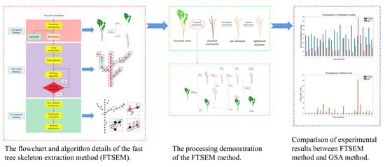
In this section, the proposed method will be systematically introduced, the flowchart of which is shown in Figure 1. The proposed method mainly includes three parts, which are leaf points filtering, tree voxel thinning, and tree skeleton building.

2.2.1. Leaf Points Filtering

As is known to all, when the TLS instrument is used to scan the tree point cloud data, the data is essentially the 3D coordinate value, intensity value, and some other information contained in the reflected laser beam. The data type and format of the woody parts and the leaf parts of the obtained point cloud data are the same, so it is impossible to directly distinguish between the woody parts and the leaf parts in the obtained data. The woody parts include the trunk and branches, which can reflect the tree skeleton information. However, the leaf points cannot provide more information about the tree structure and may hamper the construction of the tree skeleton. Therefore, it is necessary to filter out leaf points before building a tree skeleton.

In the study, we introduced the wood–leaf classification method proposed in our previous work [42] to promote tree skeleton extraction. The automated wood–leaf classification method includes two main steps. First, based on the intensity information, K-nearest neighbors, voxel point density, and voxel neighbors, the three-step classification is used to fulfill the first level of classification. Second, the wood points verification is adopted to correct some of the misclassified points to improve the classification accuracy. The wood–leaf classification method performed well on separating the wood and leaf based on the 3D tree point cloud and intensity information, with average overall accuracy (OA) and Kappa values of 0.955 and 0.8547, respectively. The classification result was demonstrated in Figure 2 using Tree 7, in which the leaf points are green and the wood points are brown. After wood–leaf classification, the wood points remained for subsequent tree skeleton extraction.

2.2.2. Tree Voxel Thinning

Due to the leaf points filtering, the tree structure is clearer in the remaining wood points which were used to construct voxels, according to the following steps.

First, the size of wood points is calculated and recorded as ($x_{length},\hspace{0.17em}{y}_{length},\hspace{0.17em}{z}_{length}$).

$$\{\begin{array}{l}{x}_{length}=x_{\max }-x_{\min }\\ y_{length}=y_{\max }-y_{\min }\\ z_{length}=z_{\max }-z_{\min }\end{array}$$

(1)

where ($x_{\min },y_{\min },z_{\min }$) and ($x_{\max },y_{\max },z_{\max }$) are the minimum and maximum values in three dimensions of voxel space.

Second, the point cloud is equally divided into n parts in each dimension. The size of a voxel $(x_{size},\hspace{0.17em}{y}_{size},\hspace{0.17em}{z}_{size})$ can be calculated using Equation (2), in which n is 100 in the experiment. In the voxel space, the voxel position is described using the number of rows, columns, and layers.

$$\{\begin{array}{l}{x}_{size}=Floor(x_{length}/n)\\ y_{size}=Floor(y_{length}/n)\\ z_{size}=Floor(z_{length}/n)\end{array}$$

(2)

where $Floor(\hspace{0.17em})$ means finding the closest smaller integer.

Third, each point is mapped to a specific voxel. The corresponding voxel coordinates $(c_x,\hspace{0.17em}{c}_y,\hspace{0.17em}{c}_z)$ of each point are calculated as Equation (3). The number of points belonging to a specific voxel is calculated to determine a wood or leaf voxel. In leaf voxels, there are small amounts of points that will make it less possible for the voxel to be a woody part. Therefore, the ratio of actual points to theoretical points in the voxel and the voxel neighborhood relationships were used to make the decision [42]. The morphological tree structure can be basically described using wood voxels.

$$\{\begin{array}{l}{c}_x=Floor((p_x-x_{\min })/x_{size})+m\\ c_y=Floor((p_y-y_{\min })/y_{size})+m\\ c_z=Floor((p_z-z_{\min })/z_{size})+m\end{array}$$

(3)

where $(p_x,p_y,p_z)$ are the coordinates of a point, m represents the m layers of empty voxels added around the existing voxel space.

Finally, a thinning algorithm [43] using 144 deletion templates with the size of 3 × 3 × 3 in the voxel space is adopted to thin the wood voxels. To ensure isotropy, six deletion directions need to be considered, such as up, down, north, east, south and west; i.e., top, bottom, back, right, front and left. The six deletion base templates for the up direction (U) are shown in Figure 3. Eighteen new deletion templates were obtained by rotating these templates clockwise (or counterclockwise, with the same result) by 90°, 180°, and 270°, respectively. There are 24 deletion templates in total for the direction U. Similarly, the deletion templates of the other five directions can be obtained by flipping the deletion templates of the direction U. All the 144 deletion templates were used to thin the wood voxels into the linear voxel tree structure.

2.2.3. Tree Skeleton Building

Building a tree skeleton can be described in three steps, which are raw skeleton construction, breakpoint connection, and skeleton optimization.

Raw Skeleton Construction

The raw skeleton is constructed based on linear voxels which mostly demonstrate the tree structure. The linking relationship between voxels is built on their neighborhood relationships.

First, calculate the barycentric coordinate $s_i$ of all points in the wood voxel $v_i$ ($i=1,\cdot \cdot \cdot ,vn$, where vn denotes the number of wood voxels) according to Equation (4). $s_i$ is defined as the skeleton node representing the voxel $v_i$.

$$s_i(x,y,z)=(\frac{{\displaystyle {\sum }_1^n{x}_j}}{n},\frac{{\displaystyle {\sum }_1^n{y}_j}}{n},\frac{{\displaystyle {\sum }_1^n{z}_j}}{n})$$

(4)

where n is the total number of points in the voxel $v_i$, and ($x_j,y_j,z_j$) is the coordinates of the point $p_j$ in the voxel $v_i$.

Second, search for the 26 neighbors of the voxel $v_i$, based on the depth-first-search (DFS) principle. Then place an undirected edge between the $v_i$ and any adjacent wood voxel, and the edge will not be allowed to be placed repeatedly. Iterate the process on each wood voxel until no more undirected edges can be placed.

Finally, the raw tree skeleton is constructed by the connection of skeleton nodes, and some skeleton nodes are linked locally, which are separated from the others, shown in Figure 4. A voxel in blue in Figure 3 represents an empty voxel in voxel space.

Breakpoint Connection

Due to the occlusion between branches and leaves in the single scan, there is some absence of tree structure information. Some branches will have some breakpoints due to these absences. Without skeleton splicing, these isolated branch skeletons will be discarded due to separation from the main part, even though they have some tree structure information.

To better utilize this small structure information, the breakpoint connection method is provided to joint breakpoints, which can be used to reasonably obtain a more complete tree skeleton. Based on the breakpoint connection method in 2D space [44], a novel breakpoint connection method in 3D is proposed using breakpoint distance bd and angles $\alpha ,\beta ,\gamma$.

To better explain these parameters, Figure 5 is used to demonstrate the relationship, in which A and B are two breakpoints waiting for a connection.

Breakpoint distance bd: is the Euclidean geometric distance between two breakpoints A and B. The possibility of connecting two breakpoints is inversely proportional to the distance bd. The farther the distance is, the less likely it is to connect together.

As shown in Figure 5, breakpoint A and its two closest linked neighbor skeleton nodes C and D can fit a line vector $\overrightarrow{m}$. Similarly, breakpoint B and its two closest linked neighbor skeleton nodes E and F can fit a line vector $\overrightarrow{n}$. All the six skeleton nodes can fit a line vector $\overrightarrow{l}$.

$\alpha$: is the angle between $\overrightarrow{m}$ and $\overrightarrow{n}$, which is an obtuse angle. The possibility of connecting two breakpoints is proportional to the angle $\alpha$. The larger the $\alpha$, the greater the possibility of connection.

$\beta$: is the angle between $\overrightarrow{m}$ and $\overrightarrow{l}$, which is an obtuse angle. The possibility of connecting two breakpoints is proportional to the angle $\beta$. The larger the $\beta$, the greater the possibility of connection.

$\gamma$: is the angle between $\overrightarrow{n}$ and $\overrightarrow{l}$, which is an acute angle. The possibility of connecting two breakpoints is inversely proportional to the angle $\gamma$. The larger the $\gamma$, the smaller the possibility of connection.

Now we need to determine the main branch and the connection order in the process. First, the branches with the top two number of skeleton nodes are selected and define the branch with the lowest skeleton node as the main branch. Second, the other branches are connected to the main branch from bottom to top in turn. In each branch, the breakpoints are also considered from bottom to top in turn.

To reduce misconnections, two restrictions were preset in this method. One restriction is the number of skeleton nodes of small, separated branch skeletons. The small branch skeleton with skeleton nodes more than the threshold P_T was kept. The small branch skeleton with skeleton nodes less than P_T was not considered in the connection because they result too easily in irregular and chaotic connections [18]. P_T was set at 4 based on the trials. The other restriction is an empirical angle threshold θ_T of 120° set for the three angles in the process. The specific use of two restrictions is described in detail in following steps.

Step 1: Obtain a branch B_i, in branch list ($i=1,\cdot \cdot \cdot ,n$, where n denotes the number of branches). If the skeleton nodes of B_i are more than P_T, move forward to Step 2; otherwise, repeat Step 1.

Step 2: Find the 5 nearest breakpoints q_k ($k=1,\cdot \cdot \cdot ,5$) on the main branch for a breakpoint P_j of branch B_i ($j=1,\cdot \cdot \cdot ,m$, where m denotes the number of breakpoints in B_i).

Step 3: Try to find the nearest skeleton node np on the main branch for a breakpoint P_j of branch B_i, where the angle $\alpha$ is more than the threshold θ_T. Whether the skeleton node np is found or not, move to the next step.

Step 4: Calculate the $b{d}_k$, $\cos {\alpha }_k$, $\cos {\beta }_k$, and $\cos {\gamma }_k$ between P_j and q_k. If np is found, calculate the $b{d}_{np}$, $\cos {\alpha }_{np}$ between P_j and np.

Step 5: Determine if the angle properties of breakpoints q_k meet the requirements set in Equation (5). If there are some $q_{k^{\prime }}\hspace{0.17em}(q_{k^{\prime }}\subseteq q_k)$ that meet Equation (5), go to Step 6. If all q_k fail on Equation (5) and do not find np, the branch B_i will not be connected and return to Step 1. If all q_k fail on Equation (5) but find np, connect P_j and np directly, and return to Step 1.

$$\{\begin{array}{l}\cos {\alpha }_k\le \cos {\theta }_T\\ \cos {\beta }_k\le \cos {\theta }_T\\ \cos {\gamma }_k\ge \left|\cos {\theta }_T\right|\end{array}$$

(5)

Step 6: Find the breakpoint $q_{\min }$ with the smallest distance value $b{d}_{\min }$ among $q_{k^{\prime }}$ ($k^{\prime }=1,\cdot \cdot \cdot ,xn.\hspace{0.17em}xn\le 5$). If skeleton node np does not exist, connect P_j and $q_{\min }$ directly, and return to Step 1. Otherwise, connect P_j and $q_{\min }$ when $q_{\min }$ satisfies Equation (6); connect P_j and np when $q_{\min }$ fails on Equation (6). Then return to Step 1 to process the other branch skeletons.

$$\{\begin{array}{l}\cos {\alpha }_{\min }\le \cos {\alpha }_{np}\\ b{d}_{\min }\le 3·b{d}_{np}\end{array}$$

(6)

Skeleton Optimization

At this stage, the tree skeleton has basically been built. However, because the skeleton nodes are calculated according to Equation (4), the skeleton nodes are not positioned in the middle of the trunk and branches. To obtain more realistic skeleton nodes, a center fitting process is adopted for the skeleton nodes. The raw wood points are sliced at the position of skeleton node P_i to obtain a center using the circle–ellipse fitting method [45]. Subsequently, the Laplacian smoothing is adopted to improve the smoothness and the aesthetics of the tree skeleton (green points in Figure 5).

3. Results

In the experiment, twenty-four willow trees were scanned and processed to obtain tree skeletons. Each tree skeleton obtained by utilizing FTSEM is shown in Figure 6. For each tree, the subfigure (a) is the raw skeleton before breakpoint connection, and the subfigure (b) is the final tree skeleton.

As shown, there are some separated parts in the sub-figure (a). More complete final tree skeletons were shown in subfigure (b), which means the breakpoint connection makes the tree skeleton better overall. Nonetheless, some trees did not obtain satisfactory skeleton results as expected, such as Tree 10, Tree 13, and Tree 17. Tree 10 and Tree 17 have many incorrect connections in the final tree skeletons because of unsatisfactory wood–leaf classification results. In the case of Tree 13, when zoomed in to observe the detail, a skeleton with numerous burrs is shown. Tree 1, Tree 18, and Tree 21 also have minor wrong connections.

To evaluate the performance and efficiency of the proposed method, the graph search algorithm (GSA) [11] was used to extract the same tree skeletons. As shown in Figure 7, the tree skeletons obtained using GSA are not as good as the results of FTSEM. Due to the manual selection of multiple parameters in the GSA method, it is tough to obtain excellent skeleton results for each tree. Therefore, some tree skeletons were incomplete, such as Tree 1, Tree 4, Tree 10, Tree 12, Tree 17, and Tree 21. The other tree skeletons tangled with many of the twig skeletons, which are hard to verify, for example, Tree 6, Tree 7, Tree 9, Tree 14, Tree 19, and Tree 23. Tree 13 even failed to extract tree skeletons from tree point cloud data.

To better analyze the proposed method, the number of skeleton nodes and the time cost of each tree using two methods were recorded in

Table 2. The information on twenty-four tree skeletons using FTSEM and GSA.

Tree Number	Point Number	Node Number		Runtime (s)		TPMP (s)
		FTSEM	GSA	FTSEM	GSA	FTSEM	GSA
1	876,657	477	105	1.3	6.4	1.5	7.3
2	716,701	456	146	1.2	8.1	1.7	11.3
3	629,250	513	175	1.2	8.8	1.9	14.0
4	733,233	450	101	1.3	8.7	1.8	11.9
5	1,064,546	400	199	2.2	47.0	2.1	44.2
6	971,915	374	334	1.7	27.5	1.7	28.3
7	3,398,859	497	304	6.0	87.3	1.8	25.7
8	1,162,123	592	177	1.9	20.5	1.6	17.6
9	1,068,644	372	418	1.9	54.1	1.8	50.6
10	1,210,685	354	120	1.4	8.9	1.2	7.4
11	1,318,700	593	116	2.8	41.5	2.1	31.5
12	742,280	537	125	1.2	8.0	1.6	10.8
13	203,303	709	/	1.0	/	4.9	/
14	1,896,619	395	414	3.8	67.5	2.0	35.6
15	1,080,397	487	127	1.4	9.0	1.3	8.3
16	980,776	384	137	1.1	7.3	1.1	7.4
17	841,575	700	77	1.4	7.0	1.7	8.3
18	1,357,196	398	216	2.1	27.2	1.5	20.0
19	4,925,230	457	877	13.0	309.3	2.6	62.8
20	1,716,488	479	279	4.0	82.4	2.3	48.0
21	1,275,620	651	106	1.8	17.7	1.4	13.9
22	1,301,100	433	256	1.7	21.6	1.3	16.6
23	1,315,914	650	275	2.1	27.5	1.6	20.9
24	771,395	374	189	1.2	8.6	1.6	11.1
Average TPMP (s)	/	/	/	/	/	1.8	22.3

. The time cost of each tree using FTSEM and GSA ranged from 1.0 s to 13.0 s, and from 6.4 s to 309.3 s, respectively. In the experiment, the number of tree points ranged from 203,303 to 4,925,230. Due to the different amounts of points in each tree point cloud, the runtime fluctuated dramatically. Generally, the more tree points are the more time the processing costs. The TPMP is introduced to compare the time cost of trees with different amounts of points. The TPMP of each tree using two methods was also recorded in Table 2. The TPMP of FTSEM is more stable than GSA. Obviously, FTSEM is better for time cost whether using the runtime or the TPMP.

Furthermore, in terms of structure information, FTSEM obtained more skeleton nodes for most trees than GSA, except for three trees, i.e., Tree 9, Tree 14, and Tree 19. More skeleton nodes mean more possible structure details. The above three trees had a lot of tangled twig skeletons, which may be due to the leaf points, illustrated in Figure 7.

The comparison histograms of skeleton nodes and running time are plotted in Figure 8, in which the running time of Tree 5, Tree 7, Tree 9, Tree 14, Tree 19, and Tree 20 are out of scale.

4. Discussion

In the experiment, FTSEM demonstrated good performance on tree skeleton extraction and can be evaluated from three aspects as follows.

First, the wood–leaf classification helps to improve accuracy and speed. Some previous articles discussed the impact of leaf points filtering. As we know, dense leaves can block and reflect the laser beams so that the authenticity of the branch skeleton generated on the leaf part is doubted. That is to say, it is easy to produce incorrect branch skeletons because of the leaf points [27,32]. Therefore, Bremer et al. suggested that the raw tree point cloud should be prefiltered to ensure the accuracy of the skeleton [34]. Gao et al. divided tree point clouds into branches and leaves using the Gaussian mixture model in order to extract the tree skeleton only on wood points [36]. Based on the previous studies, we studied wood–leaf classification [42] and introduced it into the tree skeleton extraction.

Second, breakpoint connection supports gaining more complete tree skeletons. As shown in Figure 6, we obtained satisfying tree skeletons from most tree point clouds. In the experiment, we shielded some small skeletons that were generated on a small number of branch points or leaf points due to the risk of wrong connections. Similarly, Xu et al. also shielded some small branch skeletons generated by small branches and leaves in the crown to avoid producing chaotic connections [18]. Based on the enhancement of our method, some broken branches were joined based on their positions and angles, and more skeleton information was obtained from the point cloud.

However, it is still a great challenge to join the breakpoints correctly in the tree point cloud. The branches are sparsely distributed in the space, and leaves are randomly distributed in the branches. The branches and leaves block each other. Some occlusions can be speculated by using FTSEM to obtain a promotion. But some breakpoints that also meet the assumption can result in wrong connections, just like Tree 1, Tree 18, and Tree 21 shown in Figure 6. For example, in the process of the breakpoint connection, the direct connection strategy of the nearest point for better connectivity may also result in a pseudo-connection that does not exist.

Tree skeleton of Tree 13 performed unexpectedly. The main reason is that Tree 13 was located far away from the scanner and the tree points were sparse. The low density of points makes the wood–leaf classification more difficult because the density difference between wood points and leaf points decreases. The density of points also affects the determination of the wood voxel and leaf voxel. Therefore, for Tree 13, the FTSEM method only obtained an unsatisfactory result while the GSA method did not even obtain a skeleton result. Making the tree skeleton method more robust to point density is important future work.

Third, voxel thinning assists in improving the processing efficiency of the FTSEM method, as shown in Table 2. Some researchers also reported the processing time of their tree skeleton extraction algorithms. Bucksch et al. extracted the skeletons of three trees, which were a simple tree with 49,669 points, an apple tree with 385,772 points, and a tulip tree with 816,670 points [32]. The processing time for the three trees was 1.1 min, 192.0 min, and 275.6 min, respectively. He et al. also extracted the skeletons of three trees and the operating time was 55.7 s for 658,423 points, 63.2 s for 821,416 points, and 48.1 s for 583,217 points [35]. Jiang et al. reported the time cost of skeletonization for 10 artificially generated trees and 9 reconstructed trees, which ranged from 15.15 s to 82.47 s [29]. However, the number of tree points is not mentioned in their article. Ai et al. extracted skeletons for a leaf-on ginkgo tree with 1,974,535 points and a leaf-off ginkgo tree with 348,868 points, and the running time was 33 min and 18 min, respectively [37].

In the light of the difference between tree points, it is not suitable to directly compare the reported time costs obtained by different tree skeleton extraction methods [37]. In our experiment, the FTSEM method and GSA method were compared by using the TPMP indicator to offset the effect of the number of points. Therefore, the TPMP of these methods was also calculated, as shown in

Table 3. The information of Bucksch’s article, He’s article, and Ai’s article.

Articles	Tree Name	Point Number	Runtime (s)	TPMP (s)	Average TPMP (s)
[32]	Simple tree	49,669	66	1328.8	17,146.4
	Apple tree	385,772	11,520	29,862.2
	Tulip tree	816,670	16,536	20,248.1
[35]	Sample 1	658,423	55.7	84.6	81.3
	Sample 2	821,416	63.2	76.9
	Sample 3	583,217	48.1	82.5
[37]	Leaf-on ginkgo tree	1,974,535	1980	1002.8	2049.3
	Leaf-off ginkgo tree	348,868	1080	3095.7

.

The TPMP of Bucksch’s method ranged from 1328.8 s to 29,862.2 s with an average value of 17,146.4 s. The TPMP of He’s method ranged from 76.9 s to 84.6 s with an average of 81.3 s. The TPMP of Ai’s method ranged from 1002.8 s to 3095.7 s with an average of 2049.3 s. As shown in Table 2, the FTSEM method obtained an average TPMP of 1.8 s for 24 trees, and the GSA method obtained an average TPMP of 22.3 s for 24 trees. Obviously, according to the TPMP, the FTSEM method is faster and more efficient.

To analyze the performance visually, the number of skeleton nodes and the time cost of these two methods on each tree point cloud were demonstrated in Figure 8. The FTSEM method obtained more nodes than the GSA method while using less time. Specifically, it took 2.2 s to extract the skeleton of Tree 5 using the FTSEM method, while it took 47 s using the GSA method, with a time ratio of 21.4.

The ratio of the time cost of the two methods has also been calculated (shown in Figure 9). It can be seen that the larger the amount of tree point cloud data is, the larger the gap between the two methods is, indicating that the algorithm proposed in this paper has significant advantages for big data.

5. Conclusions

In this paper, we have developed a novel tree skeleton extraction method on tree point clouds. The introduction of wood–leaf classification reduces the interference of leaf points. The breakpoint connection scheme provides more complete skeletons, and the voxel thinning makes the processing fast. The accurate tree skeleton is very useful for some forest studies, such as multi-scan scene registration, tree model reconstruction, and tree shape recognition and extraction. In future work, more types of tree point clouds will be tested using FTSEM. We will also carry out some deeper studies on the impacts of leaf points and twig points to obtain more complete and real tree skeletons accurately and robustly.

References

- Zhang, L.; Li, Z.; Li, A.; Liu, F. Large-Scale Urban Point Cloud Labeling and Reconstruction. ISPRS J. Photogramm. Remote Sens. 2018, 138, 86–100. [Google Scholar] [CrossRef]
- Berger, M.; Tagliasacchi, A.; Seversky, L.M.; Alliez, P.; Guennebaud, G.; Levine, J.A.; Sharf, A.; Silva, C.T. A Survey of Surface Reconstruction from Point Clouds. Comput. Graph. Forum 2017, 36, 301–329. [Google Scholar] [CrossRef] [Green Version]
- Lamb, S.; MacLean, D.; Hennigar, C.; Pitt, D. Forecasting Forest Inventory Using Imputed Tree Lists for LiDAR Grid Cells and a Tree-List Growth Model. Forests 2018, 9, 167. [Google Scholar] [CrossRef] [Green Version]
- Kandare, K.; Ørka, H.O.; Dalponte, M.; Næsset, E.; Gobakken, T. Individual Tree Crown Approach for Predicting Site Index in Boreal Forests Using Airborne Laser Scanning and Hyperspectral Data. Int. J. Appl. Earth Obs. Geoinf. 2017, 60, 72–82. [Google Scholar] [CrossRef]
- Palace, M.; Sullivan, F.B.; Ducey, M.; Herrick, C. Estimating Tropical Forest Structure Using a Terrestrial Lidar. PLoS ONE 2016, 11, e0154115. [Google Scholar] [CrossRef]
- Zheng, G.; Ma, L.; He, W.; Eitel, J.U.H.; Moskal, L.M.; Zhang, Z. Assessing the Contribution of Woody Materials to Forest Angular Gap Fraction and Effective Leaf Area Index Using Terrestrial Laser Scanning Data. IEEE Trans. Geosci. Remote Sens. 2016, 54, 1475–1487. [Google Scholar] [CrossRef]
- Olsoy, P.J.; Mitchell, J.J.; Levia, D.F.; Clark, P.E.; Glenn, N.F. Estimation of Big Sagebrush Leaf Area Index with Terrestrial Laser Scanning. Ecol. Indic. 2016, 61, 815–821. [Google Scholar] [CrossRef]
- Kong, F.; Yan, W.; Zheng, G.; Yin, H.; Cavan, G.; Zhan, W.; Zhang, N.; Cheng, L. Retrieval of Three-Dimensional Tree Canopy and Shade Using Terrestrial Laser Scanning (TLS) Data to Analyze the Cooling Effect of Vegetation. Agric. For. Meteorol. 2016, 217, 22–34. [Google Scholar] [CrossRef]
- Oveland, I.; Hauglin, M.; Gobakken, T.; Næsset, E.; Maalen-Johansen, I. Automatic Estimation of Tree Position and Stem Diameter Using a Moving Terrestrial Laser Scanner. Remote Sens. 2017, 9, 350. [Google Scholar] [CrossRef] [Green Version]
- Hauglin, M.; Astrup, R.; Gobakken, T.; Næsset, E. Estimating Single-Tree Branch Biomass of Norway Spruce with Terrestrial Laser Scanning Using Voxel-Based and Crown Dimension Features. Scand. J. For. Res. 2013, 28, 456–469. [Google Scholar] [CrossRef]
- Li, R.; Bu, G.; Wang, P. An Automatic Tree Skeleton Extracting Method Based on Point Cloud of Terrestrial Laser Scanner. Int. J. Opt. 2017, 2017, 5408503. [Google Scholar] [CrossRef] [Green Version]
- Qin, H.; Han, J.; Li, N.; Huang, H.; Chen, B. Mass-Driven Topology-Aware Curve Skeleton Extraction from Incomplete Point Clouds. IEEE Trans. Visual. Comput. Graph. 2020, 26, 2805–2817. [Google Scholar] [CrossRef] [PubMed]
- Aiteanu, F.; Klein, R. Hybrid Tree Reconstruction from Inhomogeneous Point Clouds. Vis. Comput. 2014, 30, 763–771. [Google Scholar] [CrossRef]
- Bournez, E.; Landes, T.; Saudreau, M.; Kastendeuch, P.; Najjar, G. From TLS Point Clouds to 3d Models of Trees: A Comparison of Existing Algorithms for 3d Tree Reconstruction. Int. Arch. Photogramm. Remote Sens. Spat. Inf. Sci. 2017, XLII-2/W3, 113–120. [Google Scholar] [CrossRef] [Green Version]
- Méndez, V.; Rosell-Polo, J.R.; Pascual, M.; Escolà, A. Multi-Tree Woody Structure Reconstruction from Mobile Terrestrial Laser Scanner Point Clouds Based on a Dual Neighbourhood Connectivity Graph Algorithm. Biosyst. Eng. 2016, 148, 34–47. [Google Scholar] [CrossRef] [Green Version]
- Zhang, C.; Yang, G.; Jiang, Y.; Xu, B.; Li, X.; Zhu, Y.; Lei, L.; Chen, R.; Dong, Z.; Yang, H. Apple Tree Branch Information Extraction from Terrestrial Laser Scanning and Backpack-LiDAR. Remote Sens. 2020, 12, 3592. [Google Scholar] [CrossRef]
- Calders, K.; Newnham, G.; Burt, A.; Murphy, S.; Raumonen, P.; Herold, M.; Culvenor, D.; Avitabile, V.; Disney, M.; Armston, J.; et al. Nondestructive Estimates of Above-ground Biomass Using Terrestrial Laser Scanning. Methods Ecol. Evol. 2015, 6, 198–208. [Google Scholar] [CrossRef]
- Xu, H.; Gossett, N.; Chen, B. Knowledge and Heuristic-Based Modeling of Laser-Scanned Trees. ACM Trans. Graph. 2007, 26, 19. [Google Scholar] [CrossRef]
- Yan, D.-M.; Wintz, J.; Mourrain, B.; Wang, W.; Boudon, F.; Godin, C. Efficient and Robust Reconstruction of Botanical Branching Structure from Laser Scanned Points. In Proceedings of the 2009 11th IEEE International Conference on Computer-Aided Design and Computer Graphics, Huangshan, China, 19–21 August 2009; pp. 572–575. [Google Scholar]
- Livny, Y.; Yan, F.; Olson, M.; Chen, B.; Zhang, H.; El-Sana, J. Automatic Reconstruction of Tree Skeletal Structures from Point Clouds. In ACM SIGGRAPH Asia 2010 Papers, Proceedings of the SIGGRAPH ASIA 2010, Seoul, South Korea, 15–18 December 2010; ACM Press: New York, NY, USA, 2010; p. 1. [Google Scholar]
- Su, Z.; Zhao, Y.; Zhao, C.; Guo, X.; Li, Z. Skeleton Extraction for Tree Models. Math. Comput. Model. 2011, 54, 1115–1120. [Google Scholar] [CrossRef]
- Delagrange, S.; Jauvin, C.; Rochon, P. PypeTree: A Tool for Reconstructing Tree Perennial Tissues from Point Clouds. Sensors 2014, 14, 4271–4289. [Google Scholar] [CrossRef] [Green Version]
- Verroust, A.; Lazarus, F. Extracting Skeletal Curves from 3D Scattered Data. In Proceedings of the Proceedings Shape Modeling International ‘99. International Conference on Shape Modeling and Applications, Aizu-Wakamatsu, Japan, 1–4 March 1999. [Google Scholar]
- Wang, Z.; Zhang, L.; Fang, T.; Tong, X.; Mathiopoulos, P.T.; Zhang, L.; Mei, J. A Local Structure and Direction-Aware Optimization Approach for Three-Dimensional Tree Modeling. IEEE Trans. Geosci. Remote Sens. 2016, 54, 4749–4757. [Google Scholar] [CrossRef]
- Wang, Z.; Zhang, L.; Fang, T.; Mathiopoulos, P.T.; Qu, H.; Chen, D.; Wang, Y. A Structure-Aware Global Optimization Method for Reconstructing 3-D Tree Models from Terrestrial Laser Scanning Data. IEEE Trans. Geosci. Remote Sens. 2014, 52, 5653–5669. [Google Scholar] [CrossRef]
- Hackenberg, J.; Spiecker, H.; Calders, K.; Disney, M.; Raumonen, P. SimpleTree—An Efficient Open Source Tool to Build Tree Models from TLS Clouds. Forests 2015, 6, 4245–4294. [Google Scholar] [CrossRef]
- Mei, J.; Zhang, L.; Wu, S.; Wang, Z.; Zhang, L. 3D Tree Modeling from Incomplete Point Clouds via Optimization and L1-MST. Int. J. Geogr. Inf. Sci. 2017, 31, 999–1021. [Google Scholar] [CrossRef]
- Huang, Z.; Huang, X.; Fan, J.; Eichhorn, M.; An, F.; Chen, B.; Cao, L.; Zhu, Z.; Yun, T. Retrieval of Aerodynamic Parameters in Rubber Tree Forests Based on the Computer Simulation Technique and Terrestrial Laser Scanning Data. Remote Sens. 2020, 12, 1318. [Google Scholar] [CrossRef] [Green Version]
- Jiang, A.; Liu, J.; Zhou, J.; Zhang, M. Skeleton Extraction from Point Clouds of Trees with Complex Branches via Graph Contraction. Vis. Comput. 2020, 37, 2235–2251. [Google Scholar] [CrossRef]
- Gorte, B.; Pfeifer, N. Structuring Laser-scanned Trees Using 3D Mathematical Morphology. Int. Arch. Photogramm. Remote Sens. 2004, 35, 929–933. [Google Scholar]
- Bucksch, A.; Lindenbergh, R. CAMPINO—A Skeletonization Method for Point Cloud Processing. ISPRS J. Photogramm. Remote Sens. 2008, 63, 115–127. [Google Scholar] [CrossRef]
- Bucksch, A.; Lindenbergh, R.; Menenti, M. SkelTre: Robust Skeleton Extraction from Imperfect Point Clouds. Vis. Comput. 2010, 26, 1283–1300. [Google Scholar] [CrossRef] [Green Version]
- Fu, L.; Liu, J.; Zhou, J.; Zhang, M.; Lin, Y. Tree Skeletonization for Raw Point Cloud Exploiting Cylindrical Shape Prior. IEEE Access 2020, 8, 27327–27341. [Google Scholar] [CrossRef]
- Bremer, M.; Rutzinger, M.; Wichmann, V. Derivation of Tree Skeletons and Error Assessment Using LiDAR Point Cloud Data of Varying Quality. ISPRS J. Photogramm. Remote Sens. 2013, 80, 39–50. [Google Scholar] [CrossRef]
- He, G.; Yang, J.; Behnke, S. Research on Geometric Features and Point Cloud Properties for Tree Skeleton Extraction. Pers. Ubiquit. Comput. 2018, 22, 903–910. [Google Scholar] [CrossRef]
- Gao, L.; Zhang, D.; Li, N.; Chen, L. Force Field Driven Skeleton Extraction Method for Point Cloud Trees. Earth Sci. Inf. 2019, 12, 161–171. [Google Scholar] [CrossRef]
- Ai, M.; Yao, Y.; Hu, Q.; Wang, Y.; Wang, W. An Automatic Tree Skeleton Extraction Approach Based on Multi-View Slicing Using Terrestrial LiDAR Scans Data. Remote Sens. 2020, 12, 3824. [Google Scholar] [CrossRef]
- Huang, H.; Wu, S.; Cohen-Or, D.; Gong, M.; Zhang, H.; Li, G.; Chen, B. L1-Medial Skeleton of Point Cloud. ACM Trans. Graph. 2013, 32, 1–8. [Google Scholar] [CrossRef] [Green Version]
- Zhou, J.; Liu, J.; Zhang, M. Curve Skeleton Extraction via K-Nearest-Neighbors Based Contraction. Int. J. Appl. Math. Comput. Sci. 2020, 30, 123–132. [Google Scholar] [CrossRef]
- Wu, S.; Wen, W.; Xiao, B.; Guo, X.; Du, J.; Wang, C.; Wang, Y. An Accurate Skeleton Extraction Approach From 3D Point Clouds of Maize Plants. Front. Plant Sci. 2019, 10, 248. [Google Scholar] [CrossRef] [Green Version]
- Xiang, L.; Bao, Y.; Tang, L.; Ortiz, D.; Salas-Fernandez, M.G. Automated Morphological Traits Extraction for Sorghum Plants via 3D Point Cloud Data Analysis. Comput. Electron. Agric. 2019, 162, 951–961. [Google Scholar] [CrossRef]
- Sun, J.; Wang, P.; Gao, Z.; Liu, Z.; Li, Y.; Gan, X.; Liu, Z. Wood-Leaf Classification of Tree Point Cloud Based on Intensity and Geometric Information. Remote Sens. 2021, 13, 4050. [Google Scholar] [CrossRef]
- Palàgyi, K.; Kuba, A. A 3D 6-Subiteration Thinning Algorithm for Extracting Medial Lines. Pattern Recognit. Lett. 1998, 19, 613–627. [Google Scholar] [CrossRef]
- Zhao, J.; Liang, G.; Yuan, Z.; Zhang, D. A New Method of Breakpoint Connection Using Curve Features for Contour Vectorization. ElAEE 2012, 18, 79–82. [Google Scholar] [CrossRef] [Green Version]
- Bu, G.; Wang, P. Adaptive Circle-Ellipse Fitting Method for Estimating Tree Diameter Based on Single Terrestrial Laser Scanning. J. Appl. Remote Sens. 2016, 10, 026040. [Google Scholar] [CrossRef]
Figure 1.
Flow chart of the FTSEM algorithm.
Figure 2.
Demonstration of wood–leaf separation result using Tree 7. Brown: wood points; Green: leaf points.
Figure 3.
Six base deletion templates in the up direction. The red center point of the deletion templates is the wood voxel that needs to be judged, the remaining red points represent wood voxel, the green points represent empty voxels, the blue points indicate that the types of voxels do not need to be considered, and the yellow points indicate that at least one of them is a wood voxel.
Figure 4.
Schematic diagram of raw skeleton construction. Red point: tree skeleton node; red line: the connection of skeleton nodes; black box: voxel containing some wood points; blue box: an empty voxel.
Figure 5.
Schematic diagram of skeleton breakpoint connection. Black point: raw skeleton node; green point: skeleton node after smoothing; red point: breakpoint; purple line: line vector ; blue line: line vector ; yellow line: line vector .
Figure 6.
The tree skeleton results of 24 willow trees using the proposed method. (a) The skeleton before breakpoint connection, (b) the final skeleton.
Figure 7.
The obtained tree skeletons of 24 trees based on the GSA algorithm. The skeleton result of each tree contains two subgraphs (left: raw tree point cloud; right: final tree skeleton).
Figure 8.
The node number and time cost comparison of FTSEM and GSA, (a) the comparison information of time cost, (b) the comparison information of node number.
Figure 9.
The time cost ratio of GSA and FTSEM.