
Air–Sea Interface Parameters and Heat Flux from Neural Network and Advanced Microwave Scanning Radiometer Observations


1
School of Marine Sciences, Nanjing University of Information Science and Technology, Nanjing 210044, China
2
Southern Marine Science and Engineering Guangdong Laboratory (Zhuhai), Zhuhai 519082, China
3
Fisheries and Oceans Canada, Bedford Institute of Oceanography, Dartmouth, NS B2Y 4A2, Canada
4
State Key Laboratory of Tropical Oceanography, South China Sea Institute of Oceanology, Chinese Academy of Sciences, Guangzhou 510301, China
*
Author to whom correspondence should be addressed.
Remote Sens. 2022, 14(10), 2364; https://doi.org/10.3390/rs14102364
Submission received: 9 April 2022
/
Revised: 5 May 2022
/
Accepted: 11 May 2022
/
Published: 13 May 2022
(This article belongs to the Special Issue Remote Sensing of the Sea Surface and the Upper Ocean)
Abstract
:We present a new approach, based on a multi-parameter back-propagation neural network (BPNN) model, to simultaneously retrieve sea surface wind speed, sea surface temperature, near-surface air temperature, and dewpoint temperature over the global oceans from the Advanced Microwave Scanning Radiometer 2 (AMSR2) onboard the Global Change Observation Mission 1st-Water (GCOM-W1). The model is trained and validated with the collocations of AMSR2 multi-channel (6.9–36.5 GHz) brightness temperatures, under both clear and cloudy conditions, and National Data Buoy Center (NDBC) and Tropical Atmosphere Ocean Project (TAO) buoy measurements along with ECMWF ERA5 reanalysis data. The root-mean-square (rms) errors of BPNN-retrieved sea surface wind speed, sea surface temperature, near-surface air temperature, and dewpoint temperature are 1.13 m/s, 1.02 °C, 1.20 °C, and 1.57 °C, respectively. The first three retrieved geophysical parameters and the estimated relative humidity from near-surface air temperature and dewpoint temperature are used to compute the sensible heat flux (SHF) and latent heat flux (LHF), using an improved bulk flux parametrization. The rms errors of the estimated SHF and LHF from BPNN-derived air–sea interface variables, and those from buoy and reanalysis data, are 18.13 W/m2 and 39.56 W/m2. We also compare SHF and LHF estimates with the Yongxing air–sea flux tower measurements in the northern South China Sea. The estimated SHF and LHF in summer and autumn periods are closer to observations than in winter and spring. The proposed method has potential to derive instantaneous air–sea interface atmospheric and oceanic parameters as well as surface sensible and latent heat fluxes from AMSR2 along-track wide swath observations.
1. Introduction
Air–sea interface key variables, such as sea surface wind speed, sea surface temperature, near-surface air temperature and dewpoint temperature, and relative humidity, play important roles in the momentum and moisture exchanges between the ocean and atmosphere. Accurate knowledge of these atmospheric and oceanic variables is critical to advance our understanding of ocean circulation, the interactions between ocean and atmosphere, the global water cycle, and the prediction of weather and climate variability. Although buoys are capable of measuring the aforementioned variables, it is difficult to obtain their spatial variability, because buoys provide only sparse observations over the global oceans. Consequently, it is vital to develop a new technique to retrieve these parameters from satellite observations.
Satellite radiometers are unique passive microwave sensors used to measure geophysical parameters at the air–sea interface with large coverage and high-temporal resolution under almost all weather conditions. The Advanced Microwave Scanning Radiometer 2 (AMSR2) is a payload of the Global Change Observation Mission 1st-Water (GCOM-W1), which provides fourteen channels of horizontally and vertically polarized (hereafter, H-pol and V-pol) brightness temperature observations from low frequency (6.9 GHz) to high frequency (89 GHz). The observed multi-channel brightness temperatures have different sensitivities to oceanic, atmospheric, and sea ice parameters. Accordingly, AMSR2 observations have been used to derive moderate and high wind speeds, sea surface temperature, atmospheric columnar water vapor, cloud liquid water content, and Arctic and Antarctic sea ice concentration using various geophysical algorithms.
A statistical-based approach has been presented to obtain sea surface temperature using AMSR2 observations acquired from twelve channels (6.9–36.5 GHz) [1]. Studies have also demonstrated the four optimal frequencies (6.9, 7.3, 10.7, and 36.5 GHz) of AMSR2 for sea surface temperature retrievals [2]. In order to use AMSR2 measurements for retrieving sea surface wind speed, an empirical regression relationship between sea surface roughness and wind speed was proposed [3]. Furthermore, the brightness temperatures of the AMSR2 low-frequency channel (6.9 GHz) were applied to derive hurricane surface wind speeds utilizing a physical-based method, because the H-pol microwave emission from this frequency is more sensitive to storm wind speeds compared to those from other frequencies [4]. A neural network algorithm was also presented to retrieve sea surface wind speeds in extratropical cyclones with AMSR2 low-frequency (6.9 and 10.7 GHz) or high-frequency (18.7, 23.8, and 36.5 GHz) observations [5]. Previous studies also attempted to retrieve sea surface specific humidity using a multivariate regression method and the AMSR for Earth Observation Satellite (AMSR-E) data [6]. Nevertheless, the forementioned methods only focus on retrieving a single sea surface oceanic or atmospheric parameter. Moreover, relevant progress has not yet been found regarding near-surface air temperature and relative humidity retrievals from AMSR2 data. Thus, it is necessary to develop an approach to simultaneously retrieve sea surface wind speed, sea surface temperature, near-surface air temperature, and dewpoint temperature using AMSR2 measurements.
Global sea surface sensible and latent fluxes play key roles on the development and evolvement of various synoptic weather events. The Coupled Ocean-Atmosphere Response Experiment (COARE) bulk formulas, such as COARE 2.5 [7], COARE 3.0 [8], and the latest COARE 3.5 [9] have been widely applied to calculate sea surface sensible heat flux (SHF) and latent heat flux (LHF), with sea surface wind speed, sea surface temperature, near-surface air temperature, and relative humidity. Based on the COARE 3.0 algorithm, daily global gridded atmosphere-ocean heat flux products with 1° × 1° spatial resolution were created from the optimal synthesis of satellite observations and atmospheric reanalysis [10]. The daily mean SHF and LHF products have been compared with those observations from the Yongxing air–sea flux tower (YXASFT) in the South China Sea (SCS), and no significant overestimation of LHF in the spring and winter was found [11]. Furthermore, the ECMWF ERA-Interim (ERA-I), the NCEP-DOE Reanalysis 2 (NECP-2), the Japanese 55-year Reanalysis (JRA55), and the Flux product in the Tropics (TropFlux) also provide SHF and LHF over global oceans. The LHF from these five heat flux products has been evaluated using buoy observations in the SCS, with the mean biases ranging from −8 to 40 W/m2 [12]. The forementioned heat flux products, however, only focus on daily mean or monthly mean SHF and LHF with coarse resolution (1°–2°). Consequently, it is desirable to derive instantaneous estimates of global sea surface SHF and LHF from satellite daily ascending and descending measurements.
In this article, we aim to develop a new approach to simultaneously retrieve four atmospheric and oceanic variables (e.g., sea surface wind speed, sea surface temperature, near-surface air temperature, and dewpoint temperature) from AMSR2 multi-channel brightness temperature observations. These geophysical parameters from the proposed method are further used to estimate SHF and LHF based on an improved bulk flux parametrization. The daily global fields of air–sea interface parameters, and sea surface sensible and latent heat fluxes, are utilized to reveal their spatial patterns and variations.
2. Materials and Methods
2.1. AMSR2 Brightness Temperature Observations
The AMSR2 is a conically scanning multi-frequency radiometer onboard the Global Change Observation Mission 1st-Water (GCOM-W1). It measures dual-polarization (H- and V-pol) radiances from the sea surface and the atmosphere of the Earth at seven frequencies (6.9, 7.3, 10.7, 18.7, 23.8, 36.5, and 89 GHz) with a large swath of 1450 km and a constant incidence angle (55°). The instrument specifications (e.g., Frequency, Beam Width, and Footprint) for AMSR2 are shown in Table 1 (AMSR2 instrument specifications). The inter-calibration of AMSR2 observed brightness temperatures has been implemented using the double difference approach with the AMSR-E and Tropical Rainfall Measuring Mission (TRMM) Microwave Imager (TMI) observations as the “ground-truth” [13,14]. In our study, we use AMSR2 Level 1B version 2.0 (GW1AM2 L1B v2.0) data released from JAXA on 23 August 2016. This product includes geographic position (longitude, latitude), data acquisition time, observed multi-channel brightness temperatures, and orbit details. The summary and description of this product are available online (https://gportal.jaxa.jp/gpr/assets/mng_upload/GCOM-W/AMSR2_Level1_Product_Format_EN.pdf, accessed on 6 March 2019). We use two low-frequency channels (6.9 and 10.7 GHz) brightness temperatures to remove the radio-frequency interference (RFI) contamination over oceans based on the following condition [15]:
where TB represents brightness temperature. We also exclude AMSR2 observations contaminated by rain (V-pol TB at 18.7 GHz is larger than 240 K). We use AMSR2 multi-channel (6.9–36.5 GHz) brightness temperatures acquired at both clear and cloudy conditions as input variables of the proposed multi-parameter BPNN model to retrieve air–sea interface oceanic and atmospheric parameters.
2.2. Buoy Measurements and Reanalysis Data
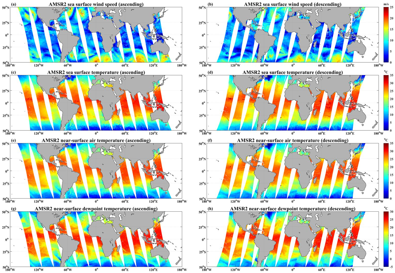
To collocate AMSR2 brightness temperature measurements, we collect buoy observations from the National Data Buoy Center (NDBC) and the Tropical Atmosphere Ocean Project (TAO) [16]. We chose a total of 94 NDBC buoys in the northwest Atlantic, northeast Pacific, Gulf of Mexico, Gulf of Alaska, and Bering Sea and 71 TAO buoys located in the equatorial regions. In order to avoid the observed brightness temperatures being contaminated by land, these selective buoys are at least 30 km far from the coast [17]. The buoy locations are illustrated in Figure 1. NDBC buoys provide hourly measurements of sea surface wind speed, sea surface temperature, near-surface air temperature, and dewpoint temperature. TAO buoys also measure these parameters and relative humidity, except for dewpoint temperature. Because NDBC buoys do not provide relative humidity measurements, we use the August-Roche-Magnus approximation [18] to estimate relative humidity with buoy-measured air temperature and dewpoint temperature.
where Td and Ta are near-surface dewpoint temperature and air temperature, respectively. RH is relative humidity.
Buoy-measured wind speeds at different heights above the ocean surface are adjusted to the equivalent neutral winds at 10 m height, utilizing a simple logarithmic wind profile equation [19]
where is the sea surface roughness length, with a constant value of 1.52 × 10⁻⁴ m assuming a drag coefficient of 1.3 × 10⁻³ [20], is the reference height of 10 m, is the height of anemometer aboard the buoy, and is the buoy-observed wind speed at height .
For the purpose of increasing the number of high wind speed data, we collect ECMWF ERA5 data over a target region (40°S–60°S, 90°E–120°E) in the Southern Ocean, because strong winds frequently exist in this area. ECMWF ERA5 is the fifth-generation atmospheric reanalysis product for investigation of the global climate and weather [21], which integrates simulations and observations into a complete and consistent global dataset based on physics laws. The users can obtain a large number of hourly estimates of atmospheric, ocean-wave, and land-surface parameters from ECMWF ERA5 data. Among these variables, we only use four geophysical parameters, namely, sea surface wind speed and temperature, near-surface air temperature, and dewpoint temperature. ECMWF ERA5 hourly data on single levels with a spatial resolution of 0.25° × 0.25° are publicly available (https://cds.climate.copernicus.eu/cdsapp#!/dataset/reanalysis-era5-single-levels?tab=form, accessed on 8 June 2019).
In this study, the AMSR2 observations acquired under clear and cloudy conditions between July 2012 and December 2020 were collocated with NDBC and TAO buoy measurements and ECMWF ERA5 reanalysis data. The temporal and spatial windows for the matchup are 30 min and 10 km, respectively. The matchup dataset includes AMSR2 brightness temperatures from twelve channels (6.9–36.5 GHz), sea surface temperature, sea surface wind speed, near-surface air temperature, and dewpoint temperature/relative humidity. We obtained a total of 137,938 pairs of AMSR2 overpasses and buoys as well as reanalysis data and randomly divided these collocation pairs into datasets T and E. These two datasets consist of 82,763 (60%) and 55,175 (40%) data pairs, respectively. We used dataset T to train the proposed multi-parameter BPNN model. Dataset E was used to evaluate the retrieved air–sea interface parameters.
2.3. Methods
2.3.1. Air–Sea Interface Parameter Retrieval
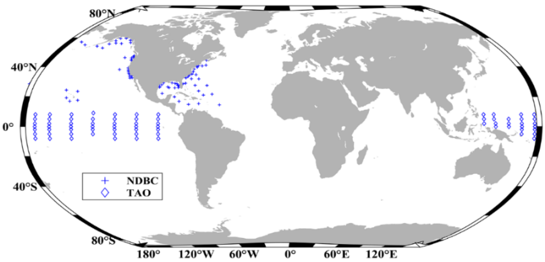
In this section, we propose a new approach, based on the three-layer multi-parameter back-propagation neural network (BPNN) model, to simultaneously retrieve four air–sea interface parameters, specifically sea surface wind speed, sea surface temperature, near-surface air temperature, and dewpoint temperature. The retrieved dewpoint temperature and air temperature are used to estimate relative humidity based on Equation (2). The BPNN model was originally designed to develop a novel learning method and thus obtain the inherent connections between input and output variables [22]. The prominent advantages of the BPNN are the incorporation of a distinctive transfer function at each neuron of the network and the utilization of the error back-propagation technique to adjust the network weights through each training procedure. The back propagation operates in a fully interconnected feed-forward neural network. In our study, the multi-parameter BPNN model is comprised of 1 input layer, 1 hidden layer, and 1 output layer. The input layer has 12 neurons that are associated with the AMSR2 brightness temperature observations from twelve channels (6.9–36.5 GHz). The hidden layer includes 30 neurons and the output layer contains 4 neurons corresponding to 4 output parameters, specifically, sea surface wind speed, sea surface temperature, near-surface air temperature, and dewpoint temperature. The architecture of the multi-parameter BPNN model for retrieval of these four geophysical parameters is illustrated in Figure 2. Each neuron in the input layer or hidden layer is linked to each of the neurons in the adjacent hidden layer or output layer. For each connection between two layers, there is a weight related to it. All weights are adjusted based on the back-propagation algorithm during the training procedure to achieve the purpose of “learning”.
Before retrieving air–sea interface parameters, we use dataset T to train the multi-parameter BPNN model. Dataset T consists of AMSR2 H- and V-pol brightness temperatures (TBs) from twelve channels, sea surface wind speed (WS), sea surface temperature (Ts), near-surface air temperature (Ta), and dewpoint temperature (Td). In terms of multi-parameter BPNN model training, WS, Ts, Ta, Td, and multi-channel TBs are input variables and targets, respectively. The training procedure includes two stages. In the first phase, the input parameters (TBs from 6.9 to 36.5 GHz) were fed into the network and propagated forward to calculate the output values (WS, Ts, Ta, Td) when accomplishing random initialization of all network weights. The BPNN model output from neuron i of layer c can be represented through an activation function (AF)
In this study, we adopt a hyperbolic tangent function as activation function.
The most notable advantage of the hyperbolic tangent function is that it produces a zero-centered output, thereby supporting the back-propagation process. Compared to a sigmoid function, the derivative of the hyperbolic tangent function is steeper and thus covers a wider range, enabling it to be more efficient, for faster learning. The ranges of and are from to and 1 to 1, respectively; denotes the input data (i.e.,) to the activation function, which is determined by neuron j of layer c – 1 as
where is the bias, is output of neuron j of layer (c − 1), is the weight of the connection between neuron I of layer c and neuron j of layer (c − 1), respectively.
In the second phase, the difference between the actual output and the desired output is estimated and spread backward via the network, thereby changing the weights in the network. The weights adjustment is based on the error of back propagation, determined through an iterative gradient descent training procedure. For each iteration, the weights are recalculated until the difference between output and target is minimal. In order to train the multi-parameter BPNN model, in a rapid and efficient manner, we use the Levenberg Marquardt (LM) algorithm [23] because it is a high-efficiency second-order nonlinear optimization technique. The learning rate is set as 0.01 during the training procedure. The multi-parameter BPNN model is trained for 348 steps to achieve convergence.
2.3.2. Sensible and Latent Flux Estimation
In this study, global air–sea interface sensible and latent fluxes are estimated from an improved bulk flux parametrization algorithm (COARE 3.5) by [9]
where SHF and LHF are sensible and latent fluxes, respectively. Here, other variables are as follows:
- is the air density at the surface;
- , are sensible heat and latent heat turbulent exchange coefficients, respectively;
- is the latent heat of vaporization and can be represented as a function of sea surface temperature (Le = (2.501 − 0.00237 × Ts) × 106);
- is the specific heat capacity of air at constant pressure (1004.67 J/kg/K);
- is the near-surface (2-m height above the sea surface) air temperature;
- is the sea surface temperature;
- is the near-surface (2-m height above the sea surface) specific humidity;
- is the saturation specific humidity at sea surface; and
- is the wind speed at 10-m height above the sea surface.
The procedure for estimating sensible and latent fluxes includes three steps. Firstly, we use the proposed multi-parameter BPNN model to retrieve sea surface wind speed, sea surface temperature, near-surface air temperature, and dewpoint temperature. Subsequently, we calculate relative humidity using retrieved air temperature and dewpoint temperature according to Equation (2). The estimated relative humidity, along with near-surface air temperature and air pressure, are used to compute specific humidity. Meanwhile, saturation specific humidity is estimated from sea surface temperature and sea surface air pressure. Finally, these geophysical parameters are further utilized to estimate sensible and latent heat fluxes based on Equations (7) and (8).
3. Results
3.1. Validation of Air–Sea Interface Parameters from BPNN
To evaluate the capability of the proposed multi-parameter BPNN model, we compare the model-retrieved sea surface wind speed, sea surface temperature, near-surface air temperature, and dewpoint temperature from AMSR2 measurements with the buoy observations and reanalysis data. Based on the collocation criteria described in Section 2.2, a total of 55,175 matchup pairs of AMSR2 and buoy and reanalysis data in dataset E are used to validate the model for global oceans from 2012 to 2020. For each data collocation pair, the brightness temperatures from twelve channels are used as input variables of the multi-parameter BPNN model and the four air–sea interface variables (WS, Ts, Ta, and Td) are determined as output parameters from the model.
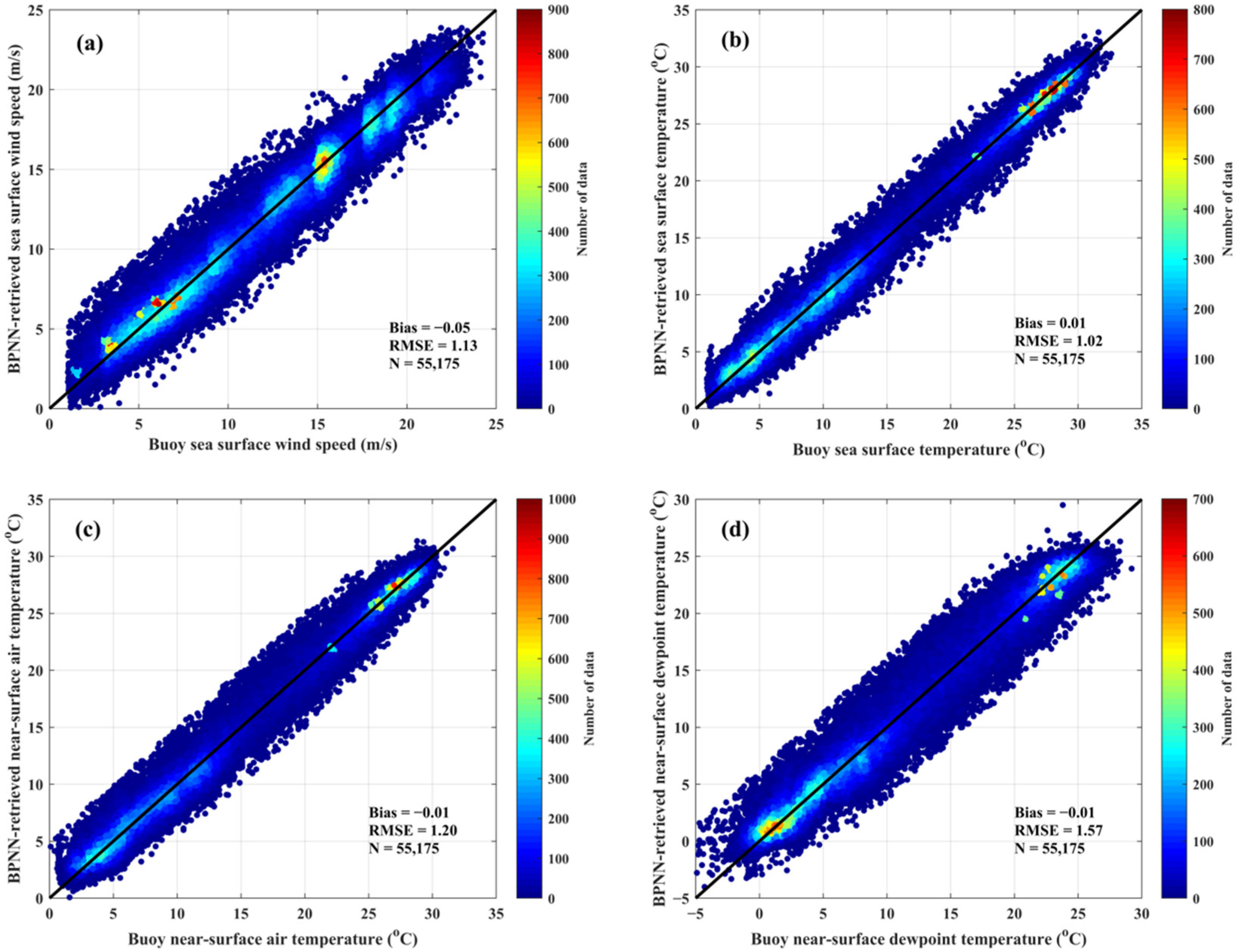
Figure 3 illustrates the comparisons between the multi-parameter BPNN model-retrieved four geophysical parameters and those from the buoy measurements and reanalysis data. As shown in Figure 3a, the bias is −0.05 m/s and the root-mean-square (rms) error is 1.13 m/s. These errors are smaller than the bias (−0.52 m/s) and the rms error (1.21 m/s) of the “Hong wind speed retrieval algorithm” [3]. The rms error of the BPNN-retrieved sea surface wind speed is close to the “standard accuracy” (1.0 m/s) specified by JAXA and much less than its “release accuracy” (1.5 m/s).
We compare BPNN-retrieved sea surface temperatures with the compound “ground-truth” (buoy observations and reanalysis data), as shown in Figure 3b. The bias and rms error are 0.01 °C and 1.02 °C, respectively, over a large dynamic range (0 °C–35 °C). The rms error is comparable to JAXA’s “release accuracy” (0.8 °C) but larger than its “standard accuracy” (0.5 °C). At very low sea surface temperatures (e.g., <3 °C), the majority of sea surface temperature retrievals are larger than “ground-truth”, which is consistent with the conclusion that the bias and the uncertainty in AMSR2 sea surface temperatures increase at lower temperature values [24]. This is probably caused by the decreasing sensitivity of brightness temperatures to sea surface temperature in cold waters [25,26].
Figure 3c shows that the BPNN-retrieved near-surface air temperatures have a small bias of –0.01 °C and an rms error of 1.2 °C. Nevertheless, the near-surface dewpoint temperature retrievals exhibit overestimates in colder waters (from –5 °C to 0 °C) and underestimates in warmer waters (from 25 °C to 30 °C), with an rms error of 1.57 °C, as shown in Figure 3d.
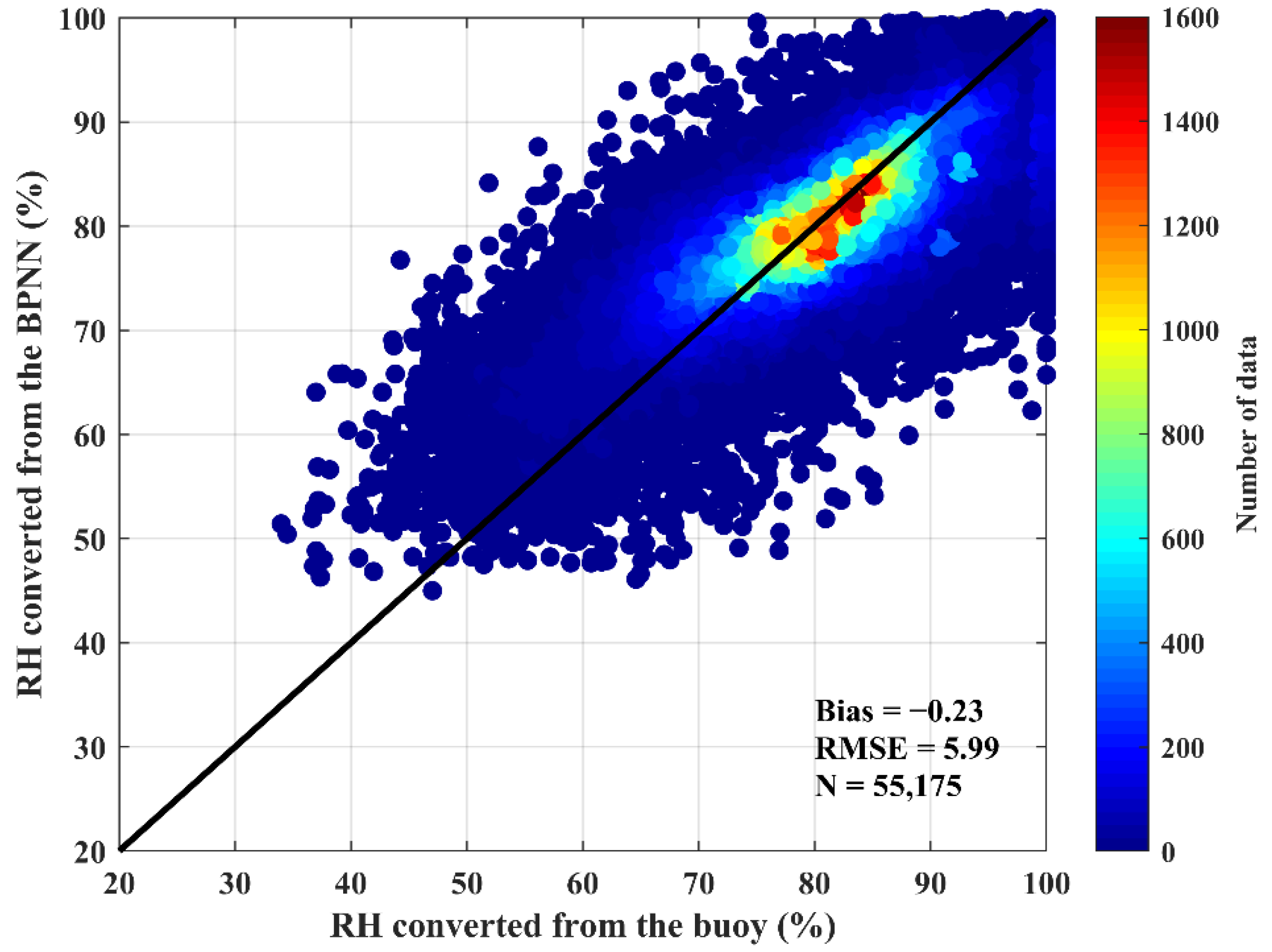
Moreover, we also use the single-parameter BPNN model to separately retrieve sea surface wind speed, sea surface temperature, near-surface air temperature, and dewpoint temperature, and the corresponding rms errors are 1.14 m/s, 1.06 °C, 1.23 °C, and 1.62 °C, respectively (not shown here). These errors are slightly larger than those derived from the multi-parameter BPNN model (1.13 m/s, 1.02 °C, 1.20 °C, and 1.57 °C). We estimate the relative humidity using the air temperature and dewpoint temperature derived from the multi-parameter BPNN model. Figure 4 shows that the bias and rms error of relative humidity are −0.23% and 5.99%, respectively, compared to buoy measurements and reanalysis data. These errors are also smaller than those obtained by a previous algorithm using SSM/I observations by [27]. Table 2 summarizes the bias and RMSE of the multi-parameter BPNN model-retrieved sea surface wind speed, sea surface temperature, near-surface air temperature and dewpoint temperature, and relative humidity.
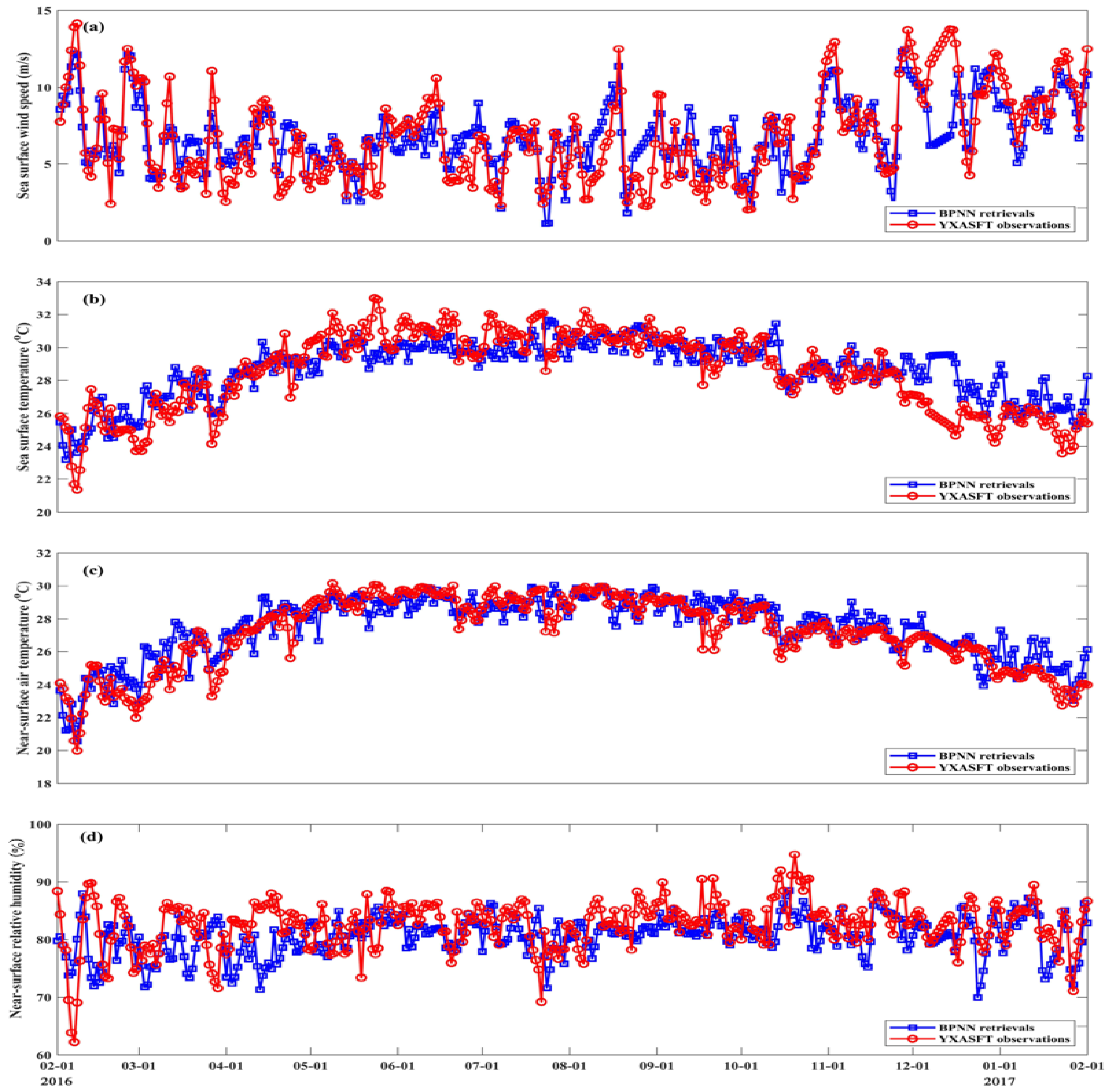
We also compare the retrievals from the multi-parameter BPNN model for sea surface wind speed, sea surface temperature, near-surface air temperature, and relative humidity with the observations from the YXASFT in the SCS. This air–sea boundary layer observation tower was installed approximately 100 m far from the northeast of Yongxing Island in the SCS [11]. There is a gradient meteorological system (GMS) on the tower which provides measurements of sea surface wind speed, sea surface temperature, near-surface air temperature and specific humidity as well as pressure. Figure 5 shows the comparisons between the BPNN retrievals and the YXASFT observations as collected during the time from 1 February 2016 to 31 January 2017. The rms errors of sea surface wind speed, sea surface temperature, near-surface air temperature, and relative humidity are 1.79 m/s, 1.72 °C, 1.41 °C, and 7.75%, respectively. The time series of YXASFT observations and BPNN retrievals show better agreement in the summer and autumn (April to November) than during winter (December to January) and spring (February to March), except for the relative humidity. In the summer and autumn periods, the high amount of atmospheric water vapor and clouds associated with the southwest monsoon in SCS may result in the large uncertainty in the relative humidity. Although BPNN-retrieved sea surface wind speed, near-surface air temperatures, and sea surface temperatures can capture the seasonal trends, they are significantly overestimated in the winter. This is possibly caused by the increased cloud cover due to the strong northeast monsoon in the northern SCS. Furthermore, the training dataset for the BPNN model does not include AMSR2 observations or buoy measurements in the SCS, which may also result in errors in the retrieved air temperatures and sea surface temperatures, especially in the winter.
3.2. Validation of Surface Heat Flux Estimates
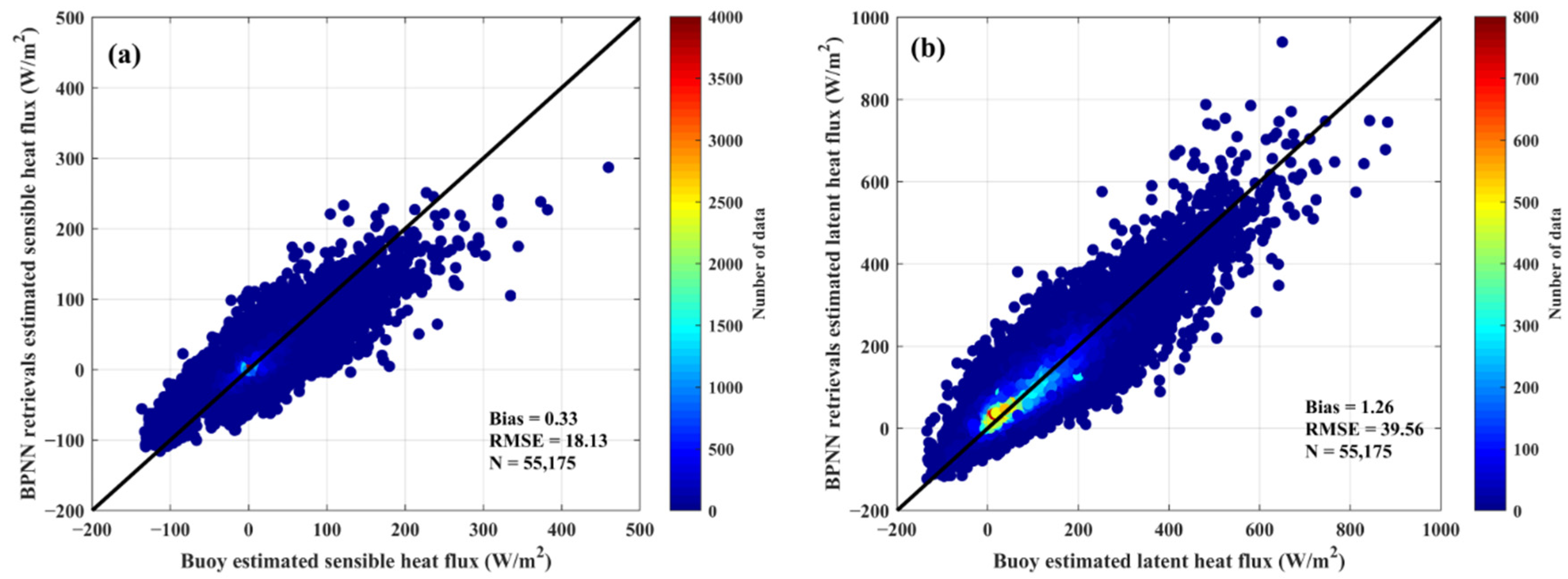
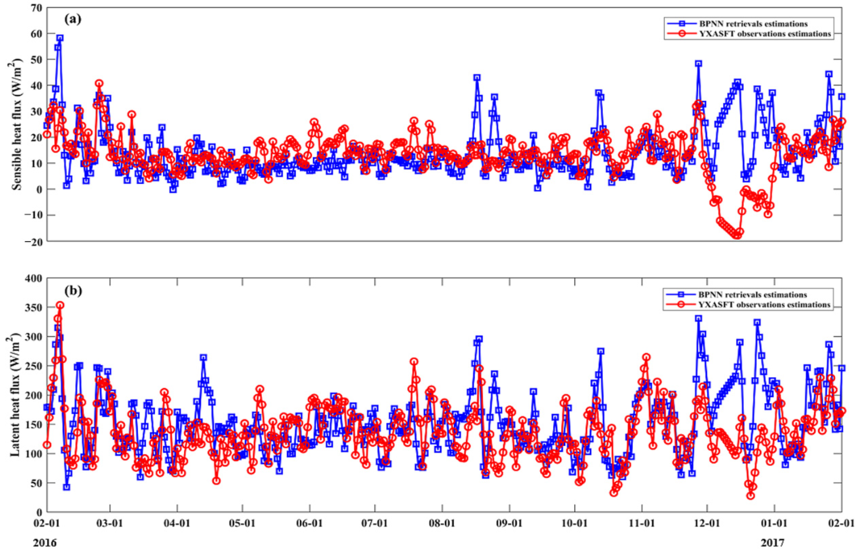
We validated the estimated sensible and latent heat fluxes against those calculations from the buoy observations and reanalysis data from 2012 to 2020 to evaluate the retrieval accuracy of the proposed method. The statistical comparison results are shown in Figure 6. The bias and rms error of the sensible heat flux are 0.33 W/m2 and 18.13 W/m2 and 1.26 W/m2 and 39.56 W/m2 for the latent heat flux. The estimated sensible heat fluxes from the COARE 3.5 and BPNN-retrieved air–sea interface parameters are underestimated when they are larger than 200 W/m2. This is very likely related to inaccurate sea surface wind speeds and air–sea temperature differences. We also compare heat flux calculations with YXASFT observations, as shown in Figure 7. The estimated sensible and latent heat fluxes in summer and autumn periods are closer to the observations than in winter and spring. The rms errors of sensible and latent heat fluxes are 9.72 W/m2 and 61.38 W/m2 in the summer–autumn period, 11.31 W/m2 and 62.92 W/m2 in the spring, and 22.32 W/m2 and 80.03 W/m2 in the winter. As discussed in Section 3.1, BPNN-retrieved sea surface temperatures and near-surface air temperatures are significantly larger than the YXASFT observations in the winter, thereby causing inaccurate air–sea temperature differences. Furthermore, notable discrepancies are found between BPNN-retrieved sea surface wind speeds and YXASFT measurements in early December. Consequently, distinct sensible heat flux differences exist in winter. The sea surface saturation specific humidity and near-surface air specific humidity are important variables for estimating latent heat flux. These two parameters are calculated from sea surface temperature, near-surface air temperature and relative humidity, and sea surface pressure. Thus, inaccurate sea surface temperature, near-surface air temperature, and relative humidity from BPNN lead to errors in estimated latent heat fluxes, especially in the winter period.
3.3. Global Daily Air–Sea Interface Parameters and Heat Fluxes
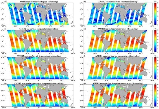
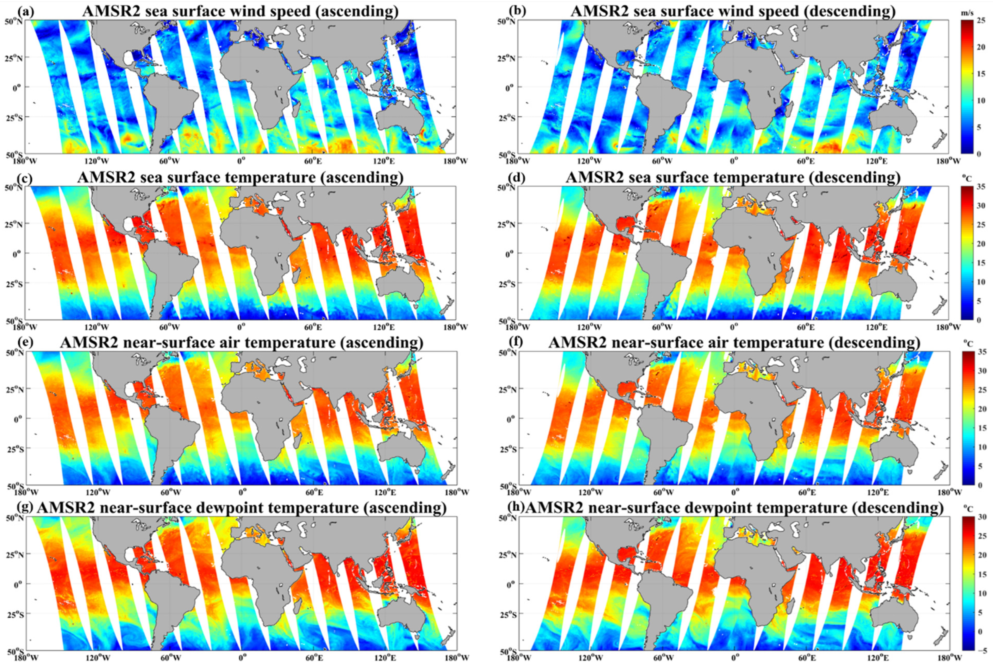
Figure 8 shows the multi-parameter BPNN model-retrieved values for the global daily instantaneous fields of sea surface wind speed, sea surface temperature, near-surface air temperature, and dewpoint temperature from AMSR2 ascending and descending brightness temperature observations for 13 July 2018. As shown in Figure 8a,b, high winds (>15 m/s) exist in the South Pacific, South Atlantic, North Atlantic, and South Indian Oceans. Figure 8c,d clearly illustrate the oceanic front features in the Kuroshio and Gulf Stream regions. On the two sides of these frontal areas, the temperature difference is about 8 °C. High sea surface temperatures (28–31 °C) exist in the northwest Pacific, North Indian Ocean, northeast Pacific, and equatorial regions. Nevertheless, we also find two distinct areas (2.1°N–4.0°S, 80.5°W–120.8°W; 1.9°N–4.0°S, 10.2°E–28.1°W) with lower sea surface temperatures (22–24 °C) in the equatorial regions. Two cold ocean currents, namely, Peru Current and Benguela Current, bring cold waters (0–6 °C) in the South Pacific and South Atlantic Oceans to these two areas, thereby causing lower sea surface temperatures. Furthermore, two cold subarctic ocean currents (Oyashio Current and Labrador Current) transport cold water from Arctic Ocean waters to areas northeast of Japan and Newfoundland, leading to very low sea surface temperatures (~4.5 °C). Near-surface air temperature and dewpoint temperature also show similar spatial patterns with sea surface temperature over global oceans, as shown in Figure 8e–h. In the tropical oceans (23°N–23°S), the mean values of near-surface air temperature and dewpoint temperature are 25 °C and 21 °C, respectively.
Figure 9 illustrates the global daily instantaneous fields of sensible flux and latent flux estimated from COARE 3.5 and the multi-parameter BPNN model-retrieved air–sea interface parameters (WS, Ts, Ta, RH) for 13 July 2018. The patterns of sensible and latent heat fluxes exhibit spatial variability over the global oceans. Large sensible and latent heat fluxes are found in regional ocean basins of the Southern Hemisphere, corresponding to high wind speeds and large sea–air temperatures and humidity differences. The large positive heat fluxes are associated with warm ocean currents, such as Agulhas Current, Brazil Current, East Australia Current, Leeuwin Current, and South Equatorial Current, associated with the transfer of heat from the ocean to the atmosphere. In the northern hemisphere, the sensible and latent fluxes are relatively smaller in the Kuroshio and Gulf Stream regions, due to lower sea surface wind speeds and smaller vertical near-surface gradients of sea–air temperature and humidity. In high northern and southern latitude areas, near-surface air temperatures are larger than sea surface temperatures and thus result in negative, sensible heat fluxes. Furthermore, when the relatively warm air encounters a cold sea surface in these areas, air temperature decreases, thereby leading to the condensation of water vapor. Consequently, near-surface specific humidity increases and the sea–air humidity difference decreases, resulting in limited evaporation. This accounts for lower latent heat fluxes in high northern and southern latitude regions.
4. Discussion
Previous studies have evaluated the AMSR2 sea surface wind speeds using moored buoy measurements, showing a mean bias of 0.3 m/s and an rms error of 1.25 m/s, when wind speeds are between 0 and 14 m/s [28]. It is notable that, in our study, the wind speed range (0–25 m/s) for validation is much larger than that of previously mentioned references. The BPNN model has good performance in retrieving high wind speeds (15–25 m/s), with an rms error of 1.08 m/s (not shown), which may result from the synchronous retrieval of sea surface wind speeds and sea surface temperatures. Earlier studies have demonstrated that the accuracy of the retrieved sea surface wind speeds from Special Sensor Microwave/Imager (SSM/I) data can be improved when sea surface temperature is included as an additional model output, particularly at high wind speeds [29].
The differences between BPNN-retrieved sea surface temperatures and buoy measurements may be associated with several factors. Firstly, AMSR2 produces a spatial average of sea surface temperature over each individual resolution cell, whereas a buoy provides a temporal average over a single location point. Hence, a spatial-temporal sampling mismatch exists between AMSR2 and buoy data. Secondly, AMSR2 “feels” the ocean skin (a few millimeters) temperature, whereas buoys measure the bulk temperature below the sea surface, ranging from 0.2 to 1.5 m. Diurnal warming can induce temperature differences between the subsurface and surface waters in the daytime [26,28,30], especially for low winds, because in these circumstances the upper ocean is not well mixed. Thus, BPNN-retrieved sea surface temperatures may significantly differ from buoy measurements acquired at low wind speeds. Finally, AMSR2 brightness temperatures are contaminated by RFI, which affects the accuracy of the retrieved sea surface temperature. In this study, although we use a brightness temperature difference of two low-frequency channels (6.9 and 10.7 GHz) as a criterion to eliminate RFI contamination over the ocean, this influence cannot be fully removed by this operation.
The retrieval of near-surface air temperature and dewpoint temperature is a challenging task because the AMSR2 measured radiances are not from single layers but from relatively thick atmospheric layers. Furthermore, no logical vertical temperature structure exists in the atmosphere and thus, it is very difficult to obtain accurate near-surface air temperatures or dewpoint temperatures from AMSR2 observations. However, compared to ocean surface parameter retrievals from SSM/I data [27], the near-surface air temperatures from our multi-parameter BPNN model and AMSR2 multi-channel brightness temperatures have smaller bias and rms error.
In our study, the majority of TAO and NDBC buoys are located between 10°S and 50°N. To examine the dependence of retrieval errors on latitude, we divide this large area into three sub-regions (10°S–10°N, 10°N–30°N, 30°N–50°N). For each sub-region, we estimate RMSE for four air–sea interface parameters as retrieved using the multi-parameter BPNN model. The results are summarized in Table 3. It is shown that RMSE values increase with increasing latitudes. In high latitude areas, high winds are usually accompanied with excessive cloud liquid water and atmospheric vapor, along with precipitation of various intensities. These features have the potential to cause additional atmospheric attenuation of the ocean emission and lead to the large error in the retrieved high wind speed, near-surface air temperature, and dewpoint temperature. Moreover, the decreased sensitivity of brightness temperatures to sea surface temperature in cold waters results in lower retrieval accuracy in high latitude regions.
According to AMSR2 channel sensitivity analysis for oceanic and geophysical parameters (https://suzaku.eorc.jaxa.jp/GCOM_W/w_amsr2/w_amsr2_wave.html, accessed on 6 March 2019), for sea surface wind speed, the relative sensitivity to brightness changes increases with increasing frequency, even up to 40 GHz. Thus, it is reasonable to retrieve sea surface wind speed using AMSR2 brightness temperatures from twelve channels (6.9–36.5 GHz). Moreover, the low frequency (6.9 GHz) is more sensitive to sea surface temperature than medium and high frequencies. A recent study has also shown that the 6.9 GHz vertically polarized brightness temperature has the highest sensitivity to sea surface temperature [31]. In addition to 6.9 GHz, the 10.7 GHz channel is also suggested for retrieving sea surface temperature because it can be used to identify values for the brightness temperature that are contaminated by RFI. For higher frequencies (18.7–36.5 GHz), brightness temperatures become less sensitive to sea surface temperature changes, but they provide important information about the atmosphere above the sea surface. Consequently, an operational retrieval algorithm was developed for retrieving sea surface temperature, utilizing AMSR2 observations from twelve channels (6–36 GHz) [1]. Studies have shown that that multi-channel algorithm is possible to improve the retrieval accuracy of sea surface temperature and sea surface wind speed, compared to a single-channel algorithm [32]. Previous research also analyzed the sensitivity of the various microwave channels to changing atmospheric and surface conditions, based on forward radiative transfer simulations [33]. They found that the 19–50.5 GHz band shows a weak relationship with near-surface air temperature for observations exceeding 20 °C. The brightness temperatures acquired between 19 and 37 GHz are suggested for retrieving near-surface air temperature. For this frequency range, brightness temperatures are sensitive to near-surface specific humidity. We use AMSR2 brightness temperatures from different channel combinations to retrieve the four air–sea interface parameters. The bias and RMSE of each parameter are summarized in Table 4. It is shown that the smallest RMSE is achieved when using brightness temperatures from twelve channels (6.9–36.5 GHz). In view of the above analysis, in our study, we use AMSR2 brightness temperatures from twelve channels (6.9–36.5 GHz) as inputs of the multi-parameter BPNN model, to simultaneously retrieve sea surface wind speed, sea surface temperature, near-surface air temperature, and dewpoint temperature.
In our study, four air–sea interface parameters are simultaneously retrieved because they have intrinsic relations. Previous studies have revealed a strong coupling between sea surface temperatures and sea surface winds based on satellite observations [34,35]. When the cold air moves over the warm water on the sea surface, downward momentum transport leads to a decrease in atmosphere stability. Thus, the turbulence within the atmospheric boundary layer is intensified and the near-surface vertical wind shear is increased. This leads to an increase in surface winds. Conversely, diminished downward momentum transport over cooler water decouples the surface winds from the stronger winds aloft, resulting in decreased surface winds and a decline in atmospheric water vapor and cloud liquid water content.
5. Conclusions
A new method based on the multi-parameter back-propagation neural network (BPNN) model was proposed to simultaneously retrieve sea surface wind speed, sea surface temperature, near-surface air temperature, and dewpoint temperature using AMSR2 data. The input variables for the BPNN are the brightness temperatures from twelve AMSR2 channels (6.9–36.5 GHz). The retrieved air temperature and dewpoint temperature were further used to estimate relative humidity based on the August-Roche-Magnus approximation in [18]. We calculate the sensible and latent heat fluxes using an improved bulk flux parametrization (COARE 3.5) and the BPNN-retrieved sea surface wind speed, sea surface temperature, near-surface surface air temperature, and the estimated relative humidity.
We train and validate the BPNN model using NDBC and TAO buoy measurements as well as ECMWF ERA5 reanalysis data from 2012 to 2020. The rms errors for the BPNN-retrieved sea surface wind speed, sea surface temperature, near-surface air temperature, and dewpoint temperature are 1.13 m/s, 1.02 °C, 1.20 °C, and 1.57 °C, respectively. The wind speed retrieval accuracy is much less than 1.5 m/s (“release accuracy” specified by JAXA for AMSR2). Although sea surface temperature retrievals are less accurate compared to JAXA’s “release accuracy” (0.8 °C), they can be retrieved in the presence of clouds. The rms errors of sea surface wind speed, sea surface temperature, and near-surface air temperature are smaller than those derived from a previous retrieval approach using SSM/I data. This is most likely due to the incorporation of AMSR2 low-frequency (6.9, 7.3, and 10.7 GHz) brightness temperatures in the multi-parameter BPNN model. The rms errors of the sensible and latent heat fluxes are 18.13 W/m2 and 39.56 W/m2, respectively. The daily fields for sea surface wind speed, sea surface temperature, near-surface air temperature and dewpoint temperature, and the sensible and latent heat fluxes over the global oceans are used to obtain the spatial variations of these parameters.
The interdependence of physically related oceanic and atmospheric and variables was taken into account in the multi-parameter BPNN retrieval model. The model achieves a good performance for wind speed retrieval, even for high winds (15–25 m/s), by including sea surface temperature as an additional output. Yet, at lower sea surface temperature values, sea surface temperature retrievals are overestimated due to decreased sensitivity of AMSR2 brightness temperatures to sea surface temperature in cold waters. Furthermore, diurnal warming might induce temperature differences between surface and subsurface waters, under low wind conditions, affecting the comparison between AMRS2 sea surface temperature retrievals and buoy measurements. The present BPNN model may be further improved by adding more in situ observations from global oceans to the training dataset and incorporating water vapor and cloud liquid water as additional output.
Author Contributions
Conceptualization, B.Z.; methodology, B.Z. and X.Y.; software, X.Y.; validation, X.Y. and F.Z.; formal analysis, B.Z. and X.Y.; investigation, B.Z., X.Y., W.P. and F.Z.; data curation, X.Y. and F.Z.; writing-original draft preparation, B.Z. and X.Y.; writing-review and editing, B.Z., X.Y., W.P. and F.Z.; visualization, X.Y.; supervision, B.Z.; project administration, B.Z.; funding acquisition, B.Z. All authors have read and agreed to the published version of the manuscript.
Funding
This research was funded by the Joint Project between the National Natural Science Foundation of China and the Russian Science Foundation under Grant 42061134016 and the National Natural Science Foundation under Grant 42076181. Additional remote sensing support was provided by Canada’s SWOT (Surface Water and Ocean Topography) program, ESA’s MAXSS (MArine eXtreme Synergy of Satellites) initiative, and the Ocean Frontier Institute based at Dalhousie University in Canada.
Data Availability Statement
AMSR-2 Level 1B brightness temperature data are freely available at https://suzaku.eorc.jaxa.jp. ECMWF ERA5 data can be accessed via Climate Data Store of Copernicus Climate Change Service (http://cds.climate.copernicus.eu). NDBC and TAO buoy data are publicly available at https://www.ndbc.noaa.gov and https://tao.ndbc.noaa.gov, respectively (accessed on 8 June 2019).
Acknowledgments
The authors would like to thank the National Data Buoy Center (NDBC) and Tropical Atmosphere Ocean Project (TAO) and the European Center for Medium-Range Weather Forecasts (ECMWF) for providing buoy observations and reanalysis data.
Conflicts of Interest
The authors declare no conflict of interest.
References
- Alsweiss, S.O.; Jelenak, Z.; Chang, P.S. Remote sensing of sea surface temperature using AMSR-2 measurements. IEEE J. Sel. Top. Earth Obs. Remote Sens. 2017, 10, 3948–3954. [Google Scholar] [CrossRef]
- Peason, K.; Merchant, C.; Embury, O.; Donlon, C. The role of Advanced Microwave Scanning Radiometer 2 channels within an optimal estimation scheme for sea surface temperature. Remote Sens. 2018, 10, 90. [Google Scholar] [CrossRef] [Green Version]
- Hong, S.; Seo, H.-J.; Kwon, Y.-J. A unique satellite-based sea surface wind speed algorithm and its application in tropical cyclone intensity analysis. J. Atmos. Ocean. Technol. 2016, 33, 1363–1375. [Google Scholar] [CrossRef]
- Mai, M.; Zhang, B.; Li, X.; Hwang, P.A.; Zhang, J.A. Application of AMSR-E and AMSR-2 low-frequency channel brightness temperature data for hurricane wind retrieval. IEEE Trans. Geosci. Remote Sens. 2016, 54, 4501–4512. [Google Scholar] [CrossRef]
- Zabolotskikh, E.; Mitnik, L.; Chapron, B. GCOM-W1 AMSR-2 and MetOp-A ASCAT wind speeds for the extratropical cyclones over the North Atlantic. Remote Sens. Environ. 2014, 147, 89–98. [Google Scholar] [CrossRef]
- Zong, H.; Liu, Y.; Rong, Z.; Chen, Y. Retrieval of sea surface specific humidity based on AMSR-E satellite data. Deep. Sea Res. Part I Oceanogr. Res. Pap. 2007, 54, 1189–1195. [Google Scholar] [CrossRef]
- Fairall, C.W.; Bradley, E.F.; Rogers, D.P.; Edson, J.B.; Young, G.S. Bulk parameterization of air-sea fluxes for TOGA COARE. J. Geophys. Res. 1996, 101, 3747–3764. [Google Scholar] [CrossRef]
- Fairall, C.W.; Bradley, E.F.; Hare, J.E.; Grachev, A.A.; Edson, J.B. Bulk parameterization of air-sea fluxes: Updates and verification for the COARE algorithm. J. Clim. 2003, 16, 571–591. [Google Scholar] [CrossRef]
- Edson, J.B.; Jampana, V.; Weller, R.A.; Bigorre, S.P.; Plueddemann, A.J.; Fairall, C.W.; Miller, S.D.; Mahrt, L.; Vickers, D.; Hersbach, H. On the exchange of momentum over the open ocean. J. Phys. Oceanogr. 2013, 43, 1589–1610. [Google Scholar] [CrossRef] [Green Version]
- Yu, L.; Weller, R.A. Objectively analyzed air-sea heat fluxes for the global ice-free oceans (1981–2005). Bull. Amer. Meteorol. Soc. 2007, 88, 527–539. [Google Scholar] [CrossRef] [Green Version]
- Zhou, F.; Zhang, R.; Shi, R.; Chen, J.; He, Y.; Wang, D.; Xie, Q. Evaluation of OAFlux datasets based on in situ air-sea flux tower observations over Yongxing Island in 2016. Atmos. Meas. Tech. 2018, 11, 6091–6106. [Google Scholar] [CrossRef] [Green Version]
- Wang, X.; Zhang, R.; Huang, J.; Zeng, L.; Hwang, F. Biases of five latent heat flux products and their impacts on mixed-layer temperature estimates in the South China Sea. J. Geophys. Res. 2017, 122, 5088–5104. [Google Scholar] [CrossRef]
- Alsweiss, S.O.; Jelenak, Z.; Chang, P.S.; Park, J.D.; Meyers, P. Inter-calibration results of the advanced Microwave Scanning Radiometer-2 over ocean. IEEE J. Sel. Top. Appl. Earth Observ. Remote Sens. 2015, 8, 4230–4238. [Google Scholar] [CrossRef]
- Okuyama, A.; Imaoka, K. Intercalibration of Advanced Microwave Scanning Radiometer-2 (AMSR-2) brightness temperature. IEEE Trans. Geosci. Remote Sens. 2015, 53, 4568–4577. [Google Scholar] [CrossRef]
- Wu, Y.; Weng, F. Detection and correction of AMSR-E radio-frequency interference (RFI). Acta Meteorol. Sin. 2011, 25, 669–681. [Google Scholar] [CrossRef]
- McPhaden, M.J. The tropical atmosphere ocean array is completed. Bull. Am. Meteorol. Soc. 1995, 76, 739–741. [Google Scholar] [CrossRef]
- Goodberlet, M.A.; Swift, C.T.; Wilkson, J.C. Remote sensing of ocean surface winds with the Special Sensor Microwave/Imager. J. Geophys. Res. 1989, 94, 14547–14555. [Google Scholar] [CrossRef]
- Alduchov, A.; Eskridge, R.E. Improved Magnus form approximation of saturation vapor pressure. J. Appl. Meteorol. 1996, 35, 601–609. [Google Scholar] [CrossRef]
- Mears, A.A.; Smith, D.K.; Wentz, F.J. Comparison of special sensor microwave imager and buoy-measured wind speeds from 1987 to 1997. J. Geophys. Res. Ocean. 2001, 106, 11719–11729. [Google Scholar] [CrossRef] [Green Version]
- Peixoto, J.P.; Oort, A.H. Physics of Climate; The American Institute of Physics: Woodbury, NY, USA, 1992. [Google Scholar]
- Hersbach, H.; Bell, B.; Berrisford, P.; Hirahara, S.; Horányi, A.; Muñoz-Sabater, J.; Nicolas, J.; Peubey, C.; Radu, R.; Schepers, D.; et al. The ERA5 global reanalysis. Q. J. R. Meteorol. Soc. 2020, 146, 1999–2049. [Google Scholar] [CrossRef]
- Rumelhart, D.; Hinton, G.; Williams, R. Learning representations by back-propagating errors. Nature 1986, 323, 533–536. [Google Scholar] [CrossRef]
- Hagan, M.T.; Menhaj, M.B. Training feedforward networks with the Marquardt algorithm. IEEE Trans. Neural Netw. 1994, 5, 989–993. [Google Scholar] [CrossRef] [PubMed]
- Gentemann, C.L.; Hilburn, K.A. In situ validation of sea surface temperatures from the GCOM-W1 AMSR2 RSS calibrated brightness temperatures. J. Geophys. Res. Ocean. 2014, 120, 3567–3585. [Google Scholar] [CrossRef]
- Shibata, A. Features of ocean microwave emission changed by wind at 6 GHz. J. Oceanogr. 2006, 62, 321–330. [Google Scholar] [CrossRef]
- Gentemann, A.L.; Meissner, T.; Wentz, F.J. Accuracy of satellite sea surface temperatures at 7 and 11 GHz. IEEE Trans. Geosci. Remote Sens. 2010, 48, 1009–1018. [Google Scholar] [CrossRef]
- Meng, L.; He, Y.; Wu, Y. Neural network retrieval of ocean surface parameters from SSM/I data. Mon. Weather Rev. 2007, 135, 586–597. [Google Scholar] [CrossRef]
- Hihara, T.; Kubota, M.; Okuro, A. Evaluation of sea surface temperature and wind speed observed by GCOM-W1/AMSR2 using in situ data and global products. Remote Sens. Environ. 2015, 164, 170–178. [Google Scholar] [CrossRef]
- Krasnopolsky, V.M.; Gemmill, W.H.; Breaker, L.C. A multi-parameter empirical ocean algorithm for SSM/I retrievals. Can. J. Remote Sens. 1999, 25, 486–503. [Google Scholar] [CrossRef]
- Chen, C.S.; Beardsley, R.C.; Franks, P.J.S.; Van Keuren, J. Influence of diurnal heating on stratification and residual circulation of Georges Bank. J. Geophys. Res. 2003, 108, 8008–8028. [Google Scholar] [CrossRef]
- Nielsen-Englyst, P.; Høyer, J.L.; Alerskans, E.; Pedersen, L.T.; Donlon, C. Impact of channel selection on SST retrievals from passive microwave observations. Remote Sens. Envion. 2021, 254, 112252. [Google Scholar] [CrossRef]
- Kilic, L.; Prigent, C.; Aires, F.; Boutin, J.; Heygster, G.; Tonboe, R.T.; Roquet, H.; Jimenez, C.; Donlon, C. Expected performances of the Copernicus Imaging Microwave Radiometer (CIMR) for an all-weather and high spatial resolution estimation of ocean and sea ice parameters. J. Geophys. Res. 2018, 123, 7564–7580. [Google Scholar] [CrossRef] [Green Version]
- Jackson, D.L.; Wick, G.A.; Bates, J.J. Near-surface retrieval of air temperature and specific humidity using multisensory microwave satellite observations. J. Geophys. Res. 2006, 111, D10306. [Google Scholar] [CrossRef]
- Xie, S.-P. Satellite observations of cool ocean-atmosphere interaction. Bull. Am. Meteorol. Soc. 2004, 85, 195–208. [Google Scholar] [CrossRef] [Green Version]
- Chelton, D.B.; Schlax, M.G.; Freilich, M.H.; Milliff, R.F. Satellite measurements reveal persistent small-scale feature in ocean winds. Science 2004, 303, 978–983. [Google Scholar] [CrossRef] [PubMed] [Green Version]
Figure 1.
The locations of NDBC and TAO buoys.

Figure 2.
The topological configuration of the BPNN. H and V represent horizontal and vertical polarizations (e.g., TB 6.9H stands for horizontally polarized brightness temperature at 6.9 GHz). WS, Ts, Ta, and Td represent sea surface wind speed, sea surface temperature, near-surface air temperature, and dewpoint temperature, respectively.

Figure 3.
The comparisons between BPNN retrievals from AMSR2 observations under both clear and cloudy weather conditions and those from buoy and ECMWF ERA5 data for (a) sea surface wind speed (WS), (b) sea surface temperature (Ts), (c) near-surface air temperature (Ta), and (d) near-surface dewpoint temperature (Td) over the global oceans, for 55,175 data points from 2012 to 2020. The colored bars represent the number of data points in the specific bins. The bin size is 0.5 × 0.5 m/s for (a) and 0.5 × 0.5 °C for (b–d). Each colored point is located at the center of the bin.

Figure 4.
Comparison of the estimated relative humidity (RH) from the BPNN retrieval and the buoy and ECMWF ERA5 data over the global oceans, for 55,175 data points from 2012 to 2020. The colored bars represent the number of data points in the specific bin. The bin size is 2 × 2%. Each colored point is located at the center of the bin.

Figure 5.
Daily time-series plots of the YXASFT-observed (red solid lines) and BPNN-retrieved (blue solid lines) (a) sea surface wind speed (WS), (b) sea surface temperature (Ts), (c) near-surface air temperature (Ta), and (d) relative humidity (RH) values over a period of 1 year (from 1 February 2016 to 31 January 2017).

Figure 6.
The comparison between the estimated heat fluxes from COARE 3.5 and BPNN-retrieved air–sea interface parameters (WS, Ts, Ta, RH), and those from buoy and ECMWF ERA5 data over the global oceans, for 55,175 data points from 2012 to 2020: (a) sensible and (b) latent heat flux. The colored bars represent the number of data points in the specific bin. The bin size is 5 × 5 W/m2 for (a) and 10 × 10 W/m2 for (b). Each colored point is located at the center of the bin.

Figure 7.
Daily time-series plots of the estimated heat fluxes (blue solid lines) from COARE 3.5 and BPNN−retrieved air−sea interface parameters (WS, Ts, Ta, RH) and YXASFT observations (red solid lines) over a period of 1 year (from 1 February 2016 to 31 January 2017): (a) sensible and (b) latent heat flux.

Figure 8.
The multi−parameter BPNN model retrieved the global daily instantaneous fields for sea surface wind speed (WS), sea surface temperature (Ts), near−surface air temperature (Ta), and dewpoint temperature (Td) from AMSR2 ascending and descending brightness temperature observations for 13 July 2018. Panels (a,c,e,g) represent ascending overpasses, and (b,d,f,h) stand for descending overpasses.

Figure 9.
The global daily instantaneous fields of sensible heat flux and latent heat flux estimated from COARE 3.5 and the multi−parameter BPNN model-retrieved air−sea interface parameters (WS, Ts, Ta, RH) for 13 July 2018. Panels (a,c) represent ascending overpasses, and (b,d) stand for descending overpasses.


Table 1.
AMSR2 instrument specifications.
| Frequency (GHz) | Beam Width (deg) | Footprint (Range × Azimuth) (km) |
|---|---|---|
| 6.9/7.3 | 1.8 | 35 × 62 |
| 10.7 | 1.2 | 24 × 42 |
| 18.7 | 0.65 | 14 × 22 |
| 23.8 | 0.75 | 16 × 26 |
| 36.5 | 0.35 | 7 × 12 |
| 89.0 | 0.15 | 3 × 5 |
Table 2.
The bias and root-mean-square error (RMSE) of the multi-parameter BPNN model-retrieved sea surface wind speed (WS), sea surface temperature (Ts), near-surface air temperature (Ta) and dewpoint temperature (Td), and relative humidity (RH).
Table 2.
The bias and root-mean-square error (RMSE) of the multi-parameter BPNN model-retrieved sea surface wind speed (WS), sea surface temperature (Ts), near-surface air temperature (Ta) and dewpoint temperature (Td), and relative humidity (RH).
| Parameter | Bias | RMSE |
|---|---|---|
| WS | −0.05 m/s | 1.13 m/s |
| Ts | 0.01 °C | 1.02 °C |
| Ta | −0.01 °C | 1.20 °C |
| Td | −0.01 °C | 1.57 °C |
| RH | −0.23% | 5.99% |
Table 3.
The root-mean-square error (RMSE) of multi-parameter BPNN model-retrieved sea surface wind speed (WS), sea surface temperature (Ts), near-surface air temperature (Ta), and dewpoint temperature (Td) for three geographic regions.
Table 3.
The root-mean-square error (RMSE) of multi-parameter BPNN model-retrieved sea surface wind speed (WS), sea surface temperature (Ts), near-surface air temperature (Ta), and dewpoint temperature (Td) for three geographic regions.
| Region | Parameter | RMSE |
|---|---|---|
| 10°S–10°N | WS | 0.75 m/s |
| Ts | 0.44 °C | |
| Ta | 0.54 °C | |
| Td | 1.07 °C | |
| 10°N–30°N | WS | 1.05 m/s |
| Ts | 0.80 °C | |
| Ta | 1.14 °C | |
| Td | 1.77 °C | |
| 30°N–50°N | WS | 1.37 m/s |
| Ts | 1.32 °C | |
| Ta | 1.61 °C | |
| Td | 2.17 °C |
Table 4.
The bias and root-mean-square error (RMSE) of multi-parameter BPNN model-retrieved sea surface wind speed (WS), sea surface temperature (Ts), near-surface air temperature (Ta), and dewpoint temperature (Td), using brightness temperatures from different channel combinations.
Table 4.
The bias and root-mean-square error (RMSE) of multi-parameter BPNN model-retrieved sea surface wind speed (WS), sea surface temperature (Ts), near-surface air temperature (Ta), and dewpoint temperature (Td), using brightness temperatures from different channel combinations.
| Frequency (GHz) | Parameter | Bias | RMSE |
|---|---|---|---|
| 6.9, 7.3, 10.7, 18.3, 36.5 (V- and H-pol) | WS | −0.05 m/s | 1.13 m/s |
| Ts | 0.01 °C | 1.02 °C | |
| Ta | −0.01 °C | 1.20 °C | |
| Td | −0.01 °C | 1.57 °C | |
| 6.9, 7.3, 10.7, 18.3 (V- and H-pol) | WS | −0.04 m/s | 1.20 m/s |
| Ts | 0.01 °C | 1.08 °C | |
| Ta | −0.01 °C | 1.31 °C | |
| Td | −0.01 °C | 1.66 °C | |
| 6.9, 7.3, 10.7 (V- and H-pol) | WS | −0.05 m/s | 1.24 m/s |
| Ts | −0.01 °C | 1.20 °C | |
| Ta | −0.01 °C | 1.48 °C | |
| Td | −0.02 °C | 1.91 °C |
Publisher’s Note: MDPI stays neutral with regard to jurisdictional claims in published maps and institutional affiliations. |
© 2022 by the authors. Licensee MDPI, Basel, Switzerland. This article is an open access article distributed under the terms and conditions of the Creative Commons Attribution (CC BY) license (https://creativecommons.org/licenses/by/4.0/).
Share and Cite
MDPI and ACS Style
Zhang, B.; Yu, X.; Perrie, W.; Zhou, F. Air–Sea Interface Parameters and Heat Flux from Neural Network and Advanced Microwave Scanning Radiometer Observations. Remote Sens. 2022, 14, 2364. https://doi.org/10.3390/rs14102364
AMA Style
Zhang B, Yu X, Perrie W, Zhou F. Air–Sea Interface Parameters and Heat Flux from Neural Network and Advanced Microwave Scanning Radiometer Observations. Remote Sensing. 2022; 14(10):2364. https://doi.org/10.3390/rs14102364
Chicago/Turabian StyleZhang, Biao, Xiaotong Yu, William Perrie, and Fenghua Zhou. 2022. "Air–Sea Interface Parameters and Heat Flux from Neural Network and Advanced Microwave Scanning Radiometer Observations" Remote Sensing 14, no. 10: 2364. https://doi.org/10.3390/rs14102364
Note that from the first issue of 2016, this journal uses article numbers instead of page numbers. See further details here.