
Comparison of Satellite Driven Surface Energy Balance Models in Estimating Crop Evapotranspiration in Semi-Arid to Arid Inter-Mountain Region


Agricultural and Biological Engineering Department, Institute of Food and Agricultural Sciences, University of Florida, Gainesville, FL 32611, USA
*
Author to whom correspondence should be addressed.
Remote Sens. 2021, 13(9), 1822; https://doi.org/10.3390/rs13091822
Submission received: 9 March 2021
/
Revised: 16 April 2021
/
Accepted: 5 May 2021
/
Published: 7 May 2021
(This article belongs to the Special Issue Remote Sensing of Evapotranspiration (ET) II)
Abstract
:The regional-scale estimation of crop evapotranspiration (ETc) over a heterogeneous surface is an important tool for the decision-makers in managing and allocating water resources. This is especially critical in the arid to semi-arid regions that require supplemental water due to insufficient precipitation, soil moisture, or groundwater. Over the years, various remote sensing-based surface energy balance (SEB) models have been developed to accurately estimate ETc over a regional scale. However, it is important to carry out the SEB model assessment for a particular geographical setting to ensure the suitability of a model. Thus, in this study, four commonly used and contrasting remote sensing models viz. METRIC (mapping evapotranspiration at high resolution with internalized calibration), SEBAL (surface energy balance algorithm for land), S-SEBI (simplified surface energy balance index), and SEBS (surface energy balance system) were compared and used to quantify and map the spatio-temporal variation of ETc in the semi-arid to arid inter-mountain region of Big Horn Basin, Wyoming (Landsat Path/Row: 37/29). Model estimates from 19 cloud-free Landsat 7 and 8 images were compared with the Bowen ratio energy balance system (BREBS) flux stationed in a center pivot irrigated field during 2017 (sugar beet), 2018 (dry bean), and 2019 (barley) growing seasons. The results indicated that all SEB models are effective in capturing the variation of ETc with R2 ranging in between 0.06 to 0.95 and RMSD between 0.07 to 0.15 mm h−1. Pooled data over three vegetative surfaces for three years under irrigated conditions revealed that METRIC (NSE = 0.9) performed better across all land cover types, followed by SEBS (NSE = 0.76), S-SEBI (NSE = 0.73), and SEBAL (NSE = 0.65). In general, all SEB models substantially overestimated ETc and underestimated sensible heat (H) fluxes under dry conditions when only crop residue was available at the surface. A mid-season density plot and absolute difference maps at image scale between the models showed that models involving METRIC, SEBAL, and S-SEBI are close in their estimates of daily crop evapotranspiration (ET24) with pixel-wise RMSD ranged from 0.54 to 0.76 mm d−1 and an average absolute difference across the study area ranged from 0.47 to 0.56 mm d−1. Likewise, all the SEB models underestimated the seasonal ETc, except SEBS.
1. Introduction
Recent times have seen the unsustainable utilization of water resources, leading to short- and long-term water crises. The degrading soil and water resources coupled with climate change and variability have made it inevitable to scientifically manage agricultural water [1]. In such a scenario, managing the scarce water resources to fulfill increasing demands is a challenge. The accurate quantification of ETc at local and regional scales can aid in water resource-based policy and decision making and help manage our water resources. ETc is an energy-driven process and an important component of water budget [2] and is an essential component of irrigation water requirement quantification, irrigation planning and design, soil, and hydrological modeling [3], water use efficiency [4], and carbon flux [5], amongst others.
Over time, various highly accurate ETc measurement techniques have been put forward, with each method having its purpose, advantages, and limits. Some of the widely used methods are: (a) lysimeter [6]; (b) eddy covariance [7]; (c) Bowen ratio energy balance [8]; (d) the crop coefficient approach [3]; (e) the plant monitoring (sap flow) method [9]; (f) the energy balance method [10]; and (f) the soil water balance method [11]. In general, the footprint of ETc measurement by the aforementioned methods is relatively smaller [12], which can create substantial bias when extrapolating to a regional scale. Unlike ground-based resource-intensive methods, this research will put forward the potential of measuring ETc via satellite-driven surface energy balance (SEB) models.
The SEB algorithm developed in recent years uses visible, near-infrared, and thermal spectrum of an image to calculate energy balance fluxes. SEB models can be a single source or dual source. Single source models do not consider vegetation and soil as different entities and thus, are relatively easy to perform. On the other hand, the dual-source models consider vegetation and soil as a different entity and partitioned H between soil and vegetation. Commonly used single-source models are mapping evapotranspiration at high resolution with internalized calibration (METRIC; [10,13]), surface energy balance algorithm for land (SEBAL; [14,15]), surface energy balance system (SEBS; [16,17]), operational simplified surface energy balance (SSEBop; [18]), simplified surface energy balance index (S-SEBI; [19]), and surface energy balance index (SEBI; [20]). Likewise, atmosphere land exchange inverse (ALEXI; [21]), the two-source time integrated model (TSTIM; [22]), and the two-source energy balance model (TSEB; [23]) are some of the representative dual-source models. All these SEB models differ in input data requirements and the selection of a model is dependent upon the availability of the primary inputs. In this research, four common and contrasting single source satellite-based image processing models viz. METRIC, SEBAL, S-SEBI, and SEBS were compared and used to quantify and map the spatio-temporal variation of ETc in the semi-arid to arid inter-mountain terrain of Wyoming.
The success of the METRIC algorithm is bound to choosing appropriate hot and cold pixels during H estimation [13]. METRIC is considered distinct as compared to other contemporary models as it utilizes ground-based reference evapotranspiration (ETr) values to internally calibrate during H calculation as well as to upscale instantaneous crop evapotranspiration (ETinst). The internal calibration purportedly reduces the biases in the estimation of H and reduces the effect of advection on ETc [13]. Like METRIC, SEBAL uses anchor hot and cold pixels selected within a satellite image to compute energy balance fluxes. SEBAL and METRIC models are similar in many of their assumptions. METRIC was developed based on the SEBAL model. Compared to METRIC and SEBAL, the SEBS model is based upon atmospheric turbulent fluxes and evaporative fraction () and uses various physically based equations for determining a kB−1 parameter to calculate the difference between radiometric and aerodynamic temperature [16]. The model constrains the surface heat flux in between the dry limit (latent heat (LE) = 0) and wet limit (LE is at its potential rate) of H. On the other hand, S-SEBI has the simplest algorithm of all the models compared in this research. The fact that S-SEBI requires no meteorological data and its utilization of surface temperature (Ts) vs. surface albedo (α) feature space to compute (Λ) makes it simpler than all other models. Besides, a Ts vs. α feature space plot is reported to be more suitable in heterogeneous land cover [24].
All these SEB models have been applied individually to evaluate and estimate spatial and temporal variability of ETc under different vegetative and climatic conditions [10,17,25,26,27,28]. However, limited research is concentrated in comparison of SEB models that identify a suitable model for a specific region and climatic conditions, and highlight the model benefits and inadequacies [26,29,30]. Singh and Senay [26] compared METRIC, SEBAL, SEBS, and SSEBop models using Landsat 5 and 7 images in the mid-western U.S. They reported all the four models performing well on estimating ETinst despite their differences in complexity and assumptions when model estimates were compared with three AmeriFlux cropland sites. However, METRIC and SSEBop ET24 estimates were closer with overall R2 for both models at 0.92 and RMSD at 0.93 mm d−1 and 0.84 mm d−1,respectively. A density plot between models on predicting ET24 revealed a high degree of linearity for plots involving METRIC, SEBAL, and SEBS models compared to SSEBop. Wagle et al. [30] compared five different remote sensing models viz. METRIC, SEBAL, SEBS, S-SEBI, and SSEBop on a sorghum field during the 2012 and 2013 growing seasons using 19 Landsat 7 and 8 images. They reported poor performance of METRIC (R2 = 0.71 and RMSD = 1.5 mm d−1) and SSEBop (R2 = 0.59 and RMSD = 1.24 mm d−1) as compared to SEBAL (R2 = 0.82 and RMSD = 0.97 mm d−1), SEBS (R2 = 0.69 and RMSD = 1.08 mm d−1), and S-SEBI (R2 = 0.77 and RMSD = 0.9 mm d−1) when model estimates of ET24 estimates were compared with eddy covariance-measured corresponding flux. On a seasonal basis, models overestimated evapotranspiration (ET) (ranged between 4.7% for SEBS to 30.1% for METRIC) except for S-SEBI (−14.8%) and SSEBop (−10.7%) in the 2013 growing season. Bhattarai et al. [29] also compared METRIC, SEBAL, SEBS, S-SEBI, and SSEBop in a humid subtropical climate using 149 Landsat 5 and 7 images. Their research reported the poor performance of SSEBop (R2 = 0.71 and RMSD = 1.67 mm d−1), average performance of METRIC (R2 = 0.81 and RMSD = 0.95 mm d−1), SEBAL (R2 = 0.77 and RMSD = 0.83 mm d−1), and S-SEBI (R2 = 0.75 and RMSD = 0.92 mm d−1), and good performance by SEBS (R2 = 0.82 and RMSD = 0.74 mm d−1) when model estimates were correlated with eddy covariance-measured ET24 at three vegetated sites: Blue Cypress, Citrus and Ferris Farm and BREBS-measured ET24 at Reddy Lake, Florida. Similarly, Losgedaragh and Rahimzadegan [31] performed a model evaluation of SEBS, SEBAL, and METRIC on estimating evaporation from a reservoir and its nearby agricultural land in a semi-arid climate of Iran using 16 Landsat 5 images and pan evaporation measurements as the ground truth. Their result indicated the SEBS model (R2 = 0.93 and RMSD = 0.62 mm d−1) performed better in estimating evaporation inside the reservoir (water surface) followed by METRIC (R2 = 0.57 and RMSD = 2.02 mm d−1) and SEBAL (R2 = 0.36 and RMSD = 5.1 mm d−1). However, the same study also compared model performance on estimating evaporation from a reservoir bank, which resulted in the SEBAL model (R2 = 0.85 and RMSD = 0.82 mm d−1) performing better, followed by METRIC (R2 = 0.79 and RMSD = 1.01 mm d−1) and SEBS (R2 = 0.36 and RMSD = 8.06 mm d−1). Likewise, Chirouze et al. [32] compared four satellite-based SEB models viz. S-SEBI, VIT (modified triangle method), TSEB, and SEBS to estimate ETc and the water stress of irrigated fields in semi-arid northern Mexico. Their study showed the S-SEBI model (RMSD = 117 W m−2) better predicted LE followed by TSEB (RMSD = 122 W m−2) and SEBS (RMSD = 131 W m−2). They also indicated SEB models tend to overestimate ETc and the model performance declines during low LAI and at vegetation senescence. Likewise, Liaqat and Choi [33] compared the METRIC and SEBS models using Landsat products in Northeast Asia having both flat as well as complex mountainous terrain. Both the models correlated (r) greater than 0.75 and had an RMSD of 0.88 mm d−1 and 1.03 mm d−1,respectively when estimated ET24 (unadjusted) from four different sites were compared with corresponding flux tower measurements. The study also showed a density plot comparison of estimated ET24 between METRIC and SEBS with R2 ranging between 0.87–0.92 and RMSD in between 0.2 mm d−1 to 0.3 mm d−1. A comparison of Landsat predicted ET and observed ET using the METRIC and TSEB models over a cotton field by French et al. [34] found average discrepancies less than 1.9 mm d−1 for both models.
The SEB models differ in their level of complexity, assumptions, and are developed in contrasting geographical and climatic settings. Lu et al. [35] recommend running a comparison test between models to identify the best-fit model in a climatic setting before those models are involved in decision making. This study was carried out in the semi-arid to arid region of mid-western USA surrounded by complex mountainous terrain. Unlike flat terrain, adjustments in SEB algorithms are needed with varying slopes, aspects, and elevation [10,13,36,37]. Thus, this research anticipates identifying the best fit model suitable to semi-arid to arid mountainous climatic settings. Likewise, complex models require extensive time and effort to set up and do not necessarily outperform the simpler models [38]. Similarly, the evaluation of different models helps to identify the limitations and uncertainties of a model. Therefore, the specific objectives of this study were to: (i) assess and compare the performance of METRIC, SEBAL, SEBS, and S-SEBI algorithms using Landsat imagery on estimating ETc with respect to measured ETc from the Bowen ratio energy balance system for the different vegetative surfaces in the intermountain region of Wyoming; (ii) quantify, map, and evaluate spatial and temporal distribution (daily, monthly, and seasonal) of ETc over the study region via the METRIC, SEBAL, SEBS, and S-SEBI model.
2. Materials and Methods
2.1. Study Area, Climate and Satellite Dataset, and Image Processing
The study area is situated in the Rocky Mountain region of the United States covering the majority of the Bighorn Basin, Wyoming (Landsat Path: 37 and Row: 29; Figure 1) [25]. The study area encompasses 7930 Km2 with an elevation between 1110 m to 3254 m. A total of 19 Landsat 7- Enhanced Thematic Mapper Plus (ETM+) and Landsat 8- Operational Land Imager (OLI) and thermal infrared sensor (TIRS) images (Path: 37, Row: 29) were retrieved for the 2017 (5 images), 2018 (9 images), and 2019 (5 images) growing seasons (Table 1). The majority of the study area is covered by natural vegetation (83%) comprising evergreen and deciduous forest, grassland, shrubland, and woody and herbaceous wetlands. The growing season is generally short due to a limited number of frost-free days in the year. The major soil type in the study area is sandy loam while major crops are alfalfa, barley, dry bean, sugar beet, and corn.
In general, the study area is dominated by a semi-arid to arid climate, with average annual precipitation (1981–2010) as low as 235 mm [39]. Over the study duration, substantial variations were observed in weather variables during each of the three years. Compared to long-term average values, 2017 had below-normal precipitation and higher ETr. The total seasonal P of 94 mm, 128 mm, and 218 mm was observed in 2017, 2018, and 2019, respectively. Likewise, the cumulative ETr was highest in 2017 (883 mm) followed by 2018 (820 mm), and the 2019 (794 mm) growing season. A detailed description of the study area characteristics and weather conditions were reported in Acharya et al. [25], Sharma et al. [40], and Rai et al. [41]. High quality hourly and daily weather data to estimate ETr and precipitation data were retrieved from the Wyoming Agricultural Climate Network (WACNet) weather station at the University of Wyoming, Powell Research and Extension Center (PREC), located within the Landsat scene footprint. The quality control of meteorological data was performed by the Water Resources Data System at the University of Wyoming and the data were disseminated via the WACNet website [42]. Quality control involves both automated and manual techniques. The flagged and missing datasets (failed quality control) are estimated via spatial and statistical methods to result in a complete data-set [43]. Based on the quality analyses, all climate data used over the study duration were judged to be of good quality. The meteorological condition at PREC, Wyoming on image acquisition day is provided in Table 1.
Likewise, the BREBS installed in 2017 in a center-pivot-irrigated field in PREC, Wyoming (44.46°N, 108.45°W) was used to assess the performance of the SEB model over three irrigated vegetative surfaces, i.e., sugar beet in 2017, dry bean in 2018, and barley in 2019. These crops were selected based on their high acreage, high economic value, and high irrigation demand in the intermountain region of Wyoming. In 2017, sugar beet cultivar 9418RR was planted on 8 May at 0.3 m plating depth with a planting density of 118,600 seeds per hectare and harvested on 13 October. In 2018, dry bean cultivar La Paz was planted on 5 June at 0.05 m soil depth and 0.56 row spacing at a seeding rate of 222,395 seeds per hectare and harvested on 10 September. In 2019, barley was planted on 5 April at a target planting density of 850,000 plants per hectare on 0.19-row spacing and harvested on 14 August. A thorough description of the BREBS station installed at PREC, Wyoming is provided on our precedent paper [25]. The BREBS data were closely supervised and general maintenance was provided on a regular basis (once a week). The meteorological data (e.g., air temperature, relative humidity, incoming shortwave solar radiation, wind speed) collected from BREBS underwent rigorous quality checks with comparisons with nearby weather station data. In BREBS, the accuracy of the calculated LE and H fluxes depends on the accuracy of the Bowen ratio. A negative Bowen ratio during the day and a larger Bowen ratio during sunset and sunrise indicate an error in H and/or LE fluxes. In such instances, H and LE fluxes are recalculated via bulk aerodynamic estimation techniques using wind speed and temperature gradient [44].
The SEB models convert the digital numbers (DNs) of each image pixel to comprehensible SEB fluxes. The conversion begins with the computation of top of atmosphere radiance and reflectance from the geo-rectified images using equations as provided in USGS Landsat 7 and 8 handbooks. Moreover, the data loss incurred in Landsat 7 due to scan line correction error was overcome by carrying out natural neighbor interpolation in ArcGIS 10.6. The final output images (instantaneous) were gap filled by finding the closest subsets of missing pixels from the surrounding pixels. Image processing was carried out using the ERDAS IMAGINE 2020 (Leica Geosystems GIS and Mapping, LLC, Atlanta, Georgia, USA) graphical model maker tool. Likewise, ArcMap 10.8 and R-Studio Version 1.4.1103 were employed for the presentation of analyzed images. To account for aspects, slopes, and elevation on Ts, the solar incidence angle was computed for each pixel and a lapse rate of 6.5 K km−1 was considered in all the models. METRIC additionally used a second lapse rate of 10 K km−1 in the mountainous terrain to compute elevation-corrected surface temperature (Ts_dem) [13]. A lapse rate change of 2000 m (foot of the mountain) was considered based upon the average elevation of the study area to toggle between the two lapse rates in METRIC. In addition to the above modification, Zom, wind speed, and atmospheric pressure were adjusted [13] as they appeared in the model algorithm. The digital elevation model (DEM) was used to account for slopes, aspects, and elevation in the above adjustments. In this study, a land-use map was used to estimate Zom and extract information for different land cover types during the result presentation. Table 2 provides the source of various datasets and the computation of primary and secondary inputs (intermediate outputs) needed in the SEB models.
2.2. Energy Balance Models (SEB)
The SEB models compute ETc as a residual of other energy balance fluxes viz. Rn, soil heat (G) and H [13] (Equation (1)) as:
The following section provides a brief overview of the SEB models used in this study.
2.2.1. METRIC Model and SEBAL Model
The net radiation (Rn) is derived for each pixel by deducting reflected short- (Rs↓) and longwave ((1 − εo) RL↓) as well as emitted long-wave (RL↑) from incident short- (Rs↓) and longwave (RL↓) [13].
where Rs ↓ is the incoming shortwave radiation (W m−2), RL ↓ is the incoming longwave radiation (W m−2), RL ↑ is the emitted outgoing longwave radiation (W m−2), and εo is the surface thermal emissivity (dimensionless).
For METRIC, G was empirically calculated as a G/Rn fraction using vegetation indices and surface temperature [52].
where Ts is the surface temperature in Kelvin and LAI (dimensionless) is the leaf area index.
For SEBAL, an empirical relation put forward by Bastiaanssen et al. [14] was used to compute G as:
The main feature of the METRIC and SEBAL model is the assumption of linearity between Ts and the near-surface air temperature difference [10,13,14,15]. In fact, the METRIC model was developed on the back of the SEBAL model [10,13], emphasized to accurately predict energy balance fluxes, particularly in advective conditions and undulating terrain [10,13]. The major difference between these two models lies in how anchor pixels (hot and cold pixel) are selected during H calculation. METRIC assumes a wet, well-irrigated crop surface with full cover as a cold pixel candidate, whereas a dry, bare agricultural field is its hot pixel candidate [10,13]. On the other hand, local water bodies and dry, bare agricultural fields are cold and hot pixel candidates in SEBAL, respectively [10,13,14,15]. NDVI, α, LAI, Ts, and land use map was taken into consideration while selecting the anchor pixels for both the model. In this study, a manual selection of hot and cold pixels was performed for both METRIC and SEBAL models. Both the anchor pixels were selected within a 20 km distance from the meteorological station. For METRIC, cold pixel candidates were selected from the well-irrigated densely vegetated area with the NDVI between 0.76 and 0.84, mid-season LAI higher than 3 or 4 m−2 m−2, surface albedo between 0.18 to 0.24, and comparatively lower Ts. However, for SEBAL, cold pixel candidates were picked from the nearest water body to the meteorological station. The hot pixel candidate for both the models had an NDVI less than 0.2, surface albedo between 0.17 to 0.23, and comparatively higher Ts. Thus, hot pixels were the same for METRIC and SEBAL models in all the images considered in the study. A detailed description of how the selection of hot and cold pixels is performed is presented in our companion paper [25]. For both METRIC and SEBAL, H is calculated as a function of aerodynamic observations such as wind speed at 2-m height (u2), vegetation type and roughness, and surface to air temperature differences as [13,14]:
where is the air density (kg m−3), Cp is the specific heat of the air (1004 J kg−1 K−1), dT is the near-surface air temperature difference between two reference heights Z1 and Z2, is the surface temperature (K), is the air temperature (K), and rah is the aerodynamic resistance to heat transfer (s m−1) over the vertical distance. Our companion paper, Acharya et al. [25], provides a detailed description of the METRIC algorithm as well as for H computation of the SEBAL model. Unlike SEBAL, METRIC uses ground- measured instantaneous ETr to internally calibrate the cold pixel during H calculation [10,13].
SEB models compute ETinst as residual of the surface energy balance components (Equation (7)).
where is the density of water (~1000 kg m−3) and λ refers to the latent heat of vaporization (J Kg−1). METRIC uses the reference ET fraction (ETrF) value to upscale ETinst to ET24 and periodic ETc [13]. ETrF (dimensionless) is computed as a ratio of ETinst to the ETr.
where ETr is computed using the standardized ASCE Penman-Monteith equation [53] on an hourly basis. METRIC utilizes ETrF to minimize the impact of advective heat on ETc. Likewise, ETrF is presumed to be equivalent to the crop coefficient and its values remain constant throughout the day [54]. The ET24 rate (mm d−1) is then calculated by multiplying ETrF values with hourly ETr values summed over 24 h (ETr-24) (Equation (9)).
For SEBAL ET24 is computed using and daily average net radiation. Λ is the ratio of latent heat to the energy available at the surface and denotes the fraction of energy that gets partitioned towards LE. SEB fluxes (Rn, G, H, and ETc) have considerable diurnal variation. However, the ratio of these fluxes () is reported to be relatively constant during the day [55]. Thus, Λ is being used in various SEB models to upscale ETinst to ET24.
where Rn24 is the daily average net radiation (W m−2) and G24 (assumed to be zero) is the daily average G flux (W m−2). Rn24 was computed using daily extraterrestrial solar radiation (Ra; W m−2) and daily atmospheric transmittance (τsw) [3]. This Rn24 is the same as that used in ETr computation using the ASCE Penman-Monteith equation.
Likewise, cubic spline interpolation was favored over linear interpolation [25] to interpolate ET24 to monthly and seasonal ETc. A detailed description of cubic spline interpolation [13] is also provided in our companion paper [25].
where ETcumulative (mm) represents the summation of ET24 from the first day to the last day of the month, Kc−i is the interpolated Kc for a month and ETr24i is the daily ETr summed over a month.
2.2.2. SEBS Model
Figure 2 shows the flowchart of SEB components and other intermediate parameters estimated by SEBS. For the SEBS model, Rn is computed as in Equation (2). In this study, an empirical relationship between vegetation indices and Ts as provided by Tasumi [52] was used to calculate G (Equations (3) and (4)). Unlike METRIC and SEBAL, where anchor pixels delineate the energy balance boundary conditions, the selection of hot and cold pixels is not required in the SEBS model. In SEBS, H is calculated using an iterative procedure that solves the relationships for the layers of the friction velocity, the difference between the near-surface potential air temperature (Ta) and Ts, and Monin-Obukhov length (L) which is expressed as:
where u* = (τo/)1/2 is the friction velocity, τo is the surface shear stress, is the density of air, k is von Karman’s constant, do is the zero-plane displacement height, z is the height above the surface, zom is the roughness height for momentum transfer, zoh is the scalar roughness height for heat transfer, Ψm and Ψh are stability correction functions for momentum and H transfer, Cp is the specific heat of air at constant pressure, g is the acceleration due to gravity, θv is the virtual temperature near the surface. The Paulson [56] and Webb [57] method was used to determine the roughness height for heat and momentum transfer and the stability correction function. An empirical relationship provided by Brutsaert [58] was used to compute wind speed at blending height (z) and the zero-plane displacement height (do).
Further, the SEBS algorithm utilizes relative evaporation (Λr) derived from H at dry (Hdry) and wet limits (Hwet) to compute Λ (Equations (17) and (18)), ETinst (Equation (7)), and ET24 (Equation (11)) [16]. At Hwet, evaporation occurs at a potential rate and H is at its minimum value. It is calculated using the Penman-Monteith parameterization equation [59], assuming the bulk internal resistance to be zero. Likewise, H is at its maximum value (LE = 0) at Hdry. It corresponds to fields where soil moisture is limited for evaporation to occur. Periodic ETc in SEBS is computed as in Equation (13).
2.2.3. S-SEBI Model
Figure 3 is the computational flowchart of SEB components by S-SEBI. The peculiar feature of the SSEBI model is that it does not require any meteorological data [19] and the model algorithm is also comparatively simpler. The S-SEBI model is based on the correlation observed between Ts and α (Figure 4). The concave Ts vs. α relationship is divisible into the evaporation-controlled and radiation-controlled zone. At the evaporation-controlled zone, Ts is first more or less constant and then starts to increase with increasing α value. Beyond a certain threshold value of α, Ts decreases with increasing α which is the radiative zone. This correlation is used to calculate Λ (Equations (20)–(22)).
where, TH is the temperature of a dry pixel, and TλE is the temperature of a wet pixel, ro is threshold α, ah and bh are the regression coefficients for the dry boundary, and aλE and bλE are the regression coefficients for the wet boundary. The Ts vs. α regression coefficients were computed by excluding α’s below the threshold α value at the wet boundary [19]. Threshold α (ro) distinguishes the evaporative and radiative regions of the scatterplot and corresponds to the maximum temperature of Ts vs. α relationship. Λ is then used to compute H (Equation (23)) and ETinst (Equation (7)). ET24 and periodic ETc is computed using Equations (11) and (12), respectively.
2.3. Models Validation
Model accuracy was assessed using the standard regression statistics, i.e., mean, standard deviation, and coefficient of determination (R2) along with three error-index statistics, i.e., root mean square difference (RMSD), percent bias error (PBE), and Nash–Sutcliffe’s efficiency (NSE) for estimating ETc as compared to corresponding BREBS flux as:
Besides, intercomparison between the models was carried out using density plots and an absolute difference map.
3. Results
3.1. Comparison between SEB-Estimated and BREBS-Measured Instantaneous Fluxes
To evaluate the performance of SEB models, model-estimated instantaneous fluxes are compared with corresponding BREBS fluxes measured at the BREBS flux tower footprint in the Powell Research and Extension Center, Powell, Wyoming (Figure 5 and Figure 6) using the approach described by Acharya et al. [25]. BREBS values were retracted at satellite overpass time (11:00 a.m. MST). A total of 19 different data points acquired for the three vegetative surfaces (sugar beet in 2017, dry bean 2018, and barley in 2019) along with the pooled data were used in the analyses. Table 3 provides a statistical comparison between the model-estimated and BREBS-measured ETinst. Our results indicated that all SEB models are effective in capturing the variation of ETinst with R2 ranging in between 0.06 to 0.95 and RMSD from 0.07 to 0.15 mm h−1. Pooled data over three vegetative surfaces for three years under irrigated conditions revealed that METRIC (NSE = 0.9) performed better across all land cover types, followed by SEBS (NSE = 0.76), S-SEBI (NSE = 0.73), and SEBAL (NSE = 0.65). Although no significant difference was observed between R2 values of METRIC and SEBS-estimated vs. BREBS-measured ETinst (0.91 vs. 0.87), the RMSD, NSE, and PBE of SEBS model was 27% larger, 18% lower, and 54% higher compared to the METRIC model.
Since the performance of SEB models varies with the underlying surface, this study also assessed the performance of SEB models individually for each surface. All SEB models performed poorly in 2017 over sugar beet, except the SEBS model. The scatter plot between the model-estimated vs. BREBS-measured ETinst revealed an R2 of 0.21, 0.06, 0.71, and 0.21 and an NSE of 0.2, −0.9, 0.2, and −0.2, for METRIC, SEBAL, SEBS, and S-SEBI, respectively. The regression analysis of estimated vs. measured ETinst in 2017 showed a non-significant correlation (p-value > 0.05) for all models except SEBS. A comparison of the SEB model-estimated ETinst in 2018 over the dry bean vegetative surface revealed the METRIC, SEBAL, SEBS, and S-SEBI explained 95% (RMSD = 0.07 mm h−1), 75% (RMSD = 0.13 mm h−1), 90% (RMSD = 0.14 mm h−1), and 81% (RMSD = 0.11 mm h−1) variability in measured ETinst, respectively. Similar to 2018, in 2019, METRIC (R2 = 0.80; RMSD = 0.08 mm h−1, PBE = 0.4%, NSE = 0.7) and SEBS (R2 = 0.80; RMSD = 0.09 mm h−1, PBE = 11%, NSE = 0.6) performed well compared to SEBAL (R2 = 0.61; RMSD = 0.17 mm h−1, PBE = 7.3%, NSE = −0.8) and S-SEBI (R2 = 0.44; RMSD = 0.15 mm h−1, PBE = 5.5%, NSE = −0.4), with all the models performing well over barley.
The fact that the 2018 growing season had nine images spread across the growing season can lead to disproportionally more accuracy for the dry beans as compared to sugar beet (2017 with five images) and barley (2019 with five images) (Table 1). An analysis of temporal biases towards the end of the 2018 growing season was carried out to better understand the model performance. For that, 2018 images from mid-July to September (resembling the images from 2017 and 2019) were analyzed and compared with BREBS measurements. The results revealed that METRIC, SEBAL, SEBS and S-SEBI explained 87% (RMSD = 0.09 mm h−1, NSE = 0.76), 48% (RMSD = 0.16 mm h−1, NSE = 0.20), 91% (RMSD = 0.12 mm h−1, NSE = 0.55), and 57% (RMSD = 0.15 mm h−1, NSE = 0.32) variability in measured ETinst, respectively (data not shown). A reduction in correlation statistics, i.e., R2, NSE, and higher RMSD reveal some degree of temporal biases in all models.
To further understand the variation in SEB model-derived ETinst, estimated H was compared with the BREBS-measured H (Figure 6). Overall, all models are effective in capturing the variation of H with R2 ranged from 0.69 to 0.86 and RMSD from 59 to 88 W m−2. The average SEB models estimate of H was 13%, 7%, and 5% higher for METRIC, SEBAL, and S-SEBI and 14% lower for the SEBS model as compared to ground observations (mean: 108 W m−2). However, the biggest difference in modeled and measured H was observed for SEBS (RMSD = 88 W m−2, PBE = −14%), where most of the underestimation was observed in the dry bean (35%) in 2018 and barley (10%) in the 2019 growing season after harvest.
3.2. Comparison of Estimated and Measured Monthly Crop Evapotranspiration (ETc)
In general, monthly ETc is more desirable for hydrological applications (e.g., seasonal irrigation requirement, conveyance capacities of irrigation systems, etc.) as compared to ETinst and ET24. In this study, the monthly ETc was calculated from ET24 using cubic interpolation [25]. Figure 7 depicts the performance of the SEB models on estimating the monthly ETc. For that, the model predicted monthly ETc for the 2018 growing season (May to September) were plotted against BREBS-measured corresponding flux. For all the models, moderate to high correlation was observed between measured and estimated ETc with R2 ranged from 0.70 to 0.95 and RMSD ranged from 18 mm for METRIC to 34 mm for S-SEBI. In general, all the models underestimated the seasonal ETc, except SEBS. However, METRIC stood out to be best-performing model owing to its lower RMSD (17.6 mm) and lower percentage error (−7.9%) followed by SEBS (RMSD = 25.8 mm, %error = +6.6), SEBAL (RMSD = 33 mm, %error = −29) and S-SEBI (RMSD = 34.3 mm, %error = −31). METRIC monthly ETc ranged between –38% (underestimation) in June to 18% (overestimation) in October. The over and underestimation of the estimated monthly ETc was higher when the soil surface was devoid of active leaf area cover. The dry bean at the BREBS footprint was planted on 5 June and harvested on 10 September. Similarly, overestimation (46%) was observed for SEBS-derived ETc in October after the dry bean harvest. Contrary to this, consistence underestimation ranging between 18% to 55% was observed for SEBAL and S-SEBI.
3.3. Intercomparison of SEB Model Estimated Daily Evapotranspiration (ET24)
An intercomparison of the SEB model-derived ET24 was carried out using density plots (Figure 8 and Figure 9) and absolute difference maps (Figure 10). Figure 8 reflects a concentrated range of estimated ET24 on 2018 image acquisition dates. The shape of the curve fluctuated (unimodal, bimodal, and multimodal) throughout the growing season as surface conditions changed. The study area comprises vast swathes of natural vegetation (83% of the total study area) whereas the cultivated area (14%) is limited. Bimodal peaks (one of the peaks relate to cropland and the other for natural vegetation) is observed in SEB models (especially for METRIC) in mid and late season (18 July, 11 August, 4 September, and 12 September) when crops are at full growth and the naturally vegetated area is under water stress. As expected, the distribution of density plots for all SEB models in mid-season (2 July, 18 July, 26 July, and 11 August) is more skewed toward higher ETc. Likewise, to understand the behavior of SEB-modeled fluxes at a spatial scale larger than a single tower footprint, the gridded SEB model ET24 output over the study domain was compared with each other using the density plots (Figure 9). The R2 and RMSD values were calculated from approximately 400,000 pixels randomly selected using ordinary linear regression. The mid-season density plots involving METRIC, SEBAL, and S-SEBI for 2 July 2018 showed a good degree of correlation (R2 > 0.81) (Figure 9a,b,d). METRIC and SEBAL models were comparatively much closer on their estimates of ET24 with R2 of 0.93 and RMSD of 0.54 mm d−1 (Figure 10a). The highest difference was between the S-SEBI vs. SEBS and SEBAL vs. SEBS models with RMSD of 1.21 mm d−1 and 1.15 mm d−1, respectively (Figure 9e,f).
Similarly, to further investigate the difference in ET24 estimated using different SEB models over the heterogeneous surface, the image-scale pixel-by-pixel absolute difference map on 2 July 2018 was constructed (Figure 10). The absolute difference map provides the inter-comparison of SEB models based on the distance from zero on the number line. On an image scale, the average difference ranged between 0.47 mm d−1 for METRIC–SEBAL to 1.23 mm d−1 for S-SEBI–SEBS. It was found that the METRIC–SEBAL model had a comparatively lower absolute difference followed by METRIC–S-SEBI (0.53 mm d−1). On the other hand, maps involving SEBS had greater absolute differences (1 to 1.23 mm d−1) which is consistent with the greater spread-out distribution of ET24 (Figure 10c, 10e, and 10f). Similarly, Figure 11 also reflects the absolute difference being lower in the cropped region as compared to the naturally vegetated area. The average absolute difference between the models in the cropped area ranged between 0.33 to 0.78 mm d−1, while for natural vegetation it ranged between 0.45 to 1.3 mm d−1.
3.4. Mapping Spatial Variation of SEB Model-Estimated Seasonal Evapotranspiration (ETc)
To investigate the difference in SEB models for different land use, spatial-intercomparison of the SEB models were also carried out using spatial variation of daily and seasonal ETc during the 2018 growing season. For daily ETc, one image on 11 August 2018 from the middle of the growing season was selected. Spatio-temporal variability throughout the growing season were also analyzed and added as Supplementary Materials (Figures S1–S4). For seasonal maps, images from May to September were considered (Figure 11 and Figure 12). On average, METRIC (4.7 mm d−1) estimated a higher ET24 for cropland followed by SEBS (4.1 mm d−1), S-SEBI (3.8 mm d−1), and SEBAL (3.6 mm d−1) (Figure 8). For natural vegetation (forest, shrubland, grassland, and wetlands), the average ET24 for all the models was less than 1 mm d−1,except for S-SEBI, which had an average ET24 of 1.6 mm d−1. A comparison between and within SEB model(s) throughout the growing season (spatio-temporal variability) was also performed using the ET24 maps (refer to Supplementary Materials, Figures S1–S4). At the seasonal scale, as expected, cropland observed higher ETc as compared to the naturally vegetated area. The study area received an inconsistent rainfall distribution during the 2018 growing season, where the majority of the rainfall was observed during May (49 mm) and June (49 mm) with a total rainfall of 158 mm between March to September. Likewise, coniferous forests (top right and bottom left of the image) accounted for a higher seasonal ETc as compared to other land cover types. Intermittent cloud masses (brown patches in the image) were captured above naturally vegetated areas, resulting in a higher ETc estimation as compared to surrounding vegetation. However, to extract the ETc rate (Table 4) cloud masking was performed. Comparison among SEB models revealed that SEBS had a higher estimation of seasonal ETc for all the major crops. SEBS seasonal ETc estimates were 4, 21, and 22% higher compared to METRIC, S-SEBI, and SEBAL, respectively. However, for natural vegetation, S-SEBI (291 mm) predicted higher average seasonal ETc, followed by METRIC (250 mm), SEBAL (186 mm), and SEBS (284 mm).
4. Discussion
4.1. SEB Models and Their Strengths and Limitations
This study analyzed 19 Landsat images captured during the 2017, 2018, and 2019 growing season to assess and compare the performance of the METRIC, SEBAL, SEBS, and S-SEBI algorithms in the semi-arid to arid intermountain region of Wyoming using four SEB models. The study anticipates putting forward a best suited SEB model for the region. Without a proper model comparison study, it would be unwise to choose a model and apply it for real-world application by policy and decision-makers. It is a matter of fact that SEB models can respond differently in different climatic and geographic settings. A model performing better in a humid condition might not be able to produce the same result in rather arid conditions [26,30].
Our result indicates that the SEB model-estimated fluxes (instantaneous and periodic) have a substantial differences between each other. The fact that the SEB models differ in the model structure, input data requirements, and assumptions made in the algorithm has contributed to the variability in model output. For example, METRIC and SEBAL models use CIMEC (calibration using inverse modeling of extreme conditions) calibration approach during H calculation to remove the systematic biases in the estimation of surface temperature and surface reflectance [13]. In METRIC and SEBAL, two extreme conditions (dry and wet pixels) are chosen to internally calibrate the SEB using hourly ETr. Therefore, the final ETc estimates in these models can be accurate even if other SEB components face uncertainties. However, models such as SEBS and S-SEBI do not undergo such rigorous calibration, and delineation using anchor pixels and ground-based hourly ETr. The SEBS algorithm theoretically determines the wet and dry limit for H and Λ. Likewise, S-SEBI utilizes a Ts vs. α relationship to determine the wet edge and dry edge.
In this study, the METRIC estimate of ETc was found to have a better correlation with the corresponding BREBS flux. This performance can be directly linked with the internal calibration procedure (CIMEC) performed in METRIC. SEBAL ETc estimates were lower compared to METRIC. This may be due to the difference: (i) in the selection of cold pixel between METRIC and SEBAL; (ii) use of ETrF compared to Λ to upscale ETinst to ET24 [26]. Likewise, all the SEB models overestimated ETinst, with percent biases ranging between 2.2% for SEBAL to 12.3% for SEBS. Similar overestimation in SEB-estimated ETc ranging between 8 to 32% was observed by Wagle et al. [30], who compared the performance of five SEB models viz METRIC, SEBAL, SEBS, S-SEBI, and SSEBop. They further ranked the SEBS models based on four statistical measures and concluded that S-SEBI and SEBAL performed better, followed by SEBS and METRIC. They reported that the poor performance of METRIC is due to overestimation of METRIC-estimated ETc because of drier and rainfed conditions, which is contrary to the irrigated setting used in this study. Similar to this study, the higher performance of METRIC and SEBS were observed by Singh and Senay [26] who compared METRIC, SEBAL, SEBS, and SSEBop-estimated ETc using Landsat 5 and 7 images over center-pivot irrigated continue corn and center-pivot irrigated maize–soybean rotation in mid-western U.S. The performance of METRIC was also found to be better compared to SEBS by Liaqat and Choi [33] in Northeast Asia over four different vegetative surfaces. They reported that internal calibration in METRIC helped reduce the biases in atmospheric correction and other input parameters. On the other hand, the inconsistent estimation of G and H in SEBS resulted in high ETc.
A consistent overestimation with PBE ranged from 11.4% for SEBAL to 38.3% for SEBS in 2018 is due to the fact that three images out of nine were captured when the soil surface was devoid of active leaf area (only crop residue was available at the surface). The three images resulted in a combined overestimation of 41%, 15%, 71%, and 10% for METRIC, SEBAL, SEBS, and S-SEBI compared to less than 10% overestimation when all the images within the growing season were analyzed. It has been reported [17,60] that the presence or absence of crop residue at the surface can impact the Ts, α, and emissivity, which can ultimately impact ETc. Allen et al. [10] compared METRIC-estimated ETc with lysimeter-measured ETc using eight Landsat images acquired from April to September. They reported 14% averaged absolute differences for sugar beet crop when one image date with dry bare soil was omitted. However, the difference increased to 30% when all the image dates were considered. Sharma et al. [17] reported higher overestimation in SEBS-estimated ET24 (21% in 2009–2010 in winter wheat crop season and 21% in 2011 in maize crop growing season) after harvest when only crop residue was available at the surface. Other studies [30,61] have also reported that SEB models overestimate ETc over crop residue and vegetation under dry conditions. Wagle et al. [30] found that all SEB models, i.e., METRIC, SEBAL, SEBS, S-SEBI, and SSEBop overestimate ETc when soil moisture is less than 10 percentiles and their performance improved with increasing soil moisture. It is worth pointing out that the SEB model outputs (ETinst) in this study exhibited considerable temporal biases, particularly when the model estimates from different times of the growing season were considered. For example, the BREBS tower considered in this study was installed in June 2017, which resulted in only a handful of images (five) in the mid to late growing season for analysis in 2017 (sugar beet growing season), compared to nine images in 2018 (dry bean growing season). This resulted in the skewness of data and errors in one direction, causing lower NSE and R2 values in 2017 [25].
As compared to the BREBS-measured H, a slight overestimation from METRIC and SEBAL (Figure 6) can be accounted to the internal calibration process (CIMEC), which accumulates all the biases from other variables into H estimation [13]. Similarly, slight overestimation in S-SEBI-derived H suggests that the assumption of zero evaporation over the dry edge (Figure 4) may not be valid. The fact that SEBS-derived H had a higher difference with measured H can be linked to the sensitivity of SEBS models toward temperature gradient and vegetation properties [33]. In general, SEBS does not require extreme anchor pixels in the H calculation and uses a pixel-by-pixel calculation of H, using the iterative procedure by solving the relationships for the profiles of the friction velocity (roughness parameterization) and the difference between the near-surface potential air temperature and potential surface temperature, which also questions its reliability because of inaccuracies in the temperature gradient and aerodynamics resistance length [33,62]. This also tends to under and overestimate ETinst for dense and sparsely vegetative conditions, respectively, which is also observed in this study, where SEBS under and overestimate ETinst and H, respectively, over a dense sugar beet surface in 2017, and over and underestimate ETinst and H, respectively, when only crop residue is available in 2018 [63]. These results were also supported by Liaqat and Choi [33]: they observed that a −5K difference between the absolute surface and radiometric temperature can result in 107% overestimation in ETinst by SEBS compared to 3% overestimation in ETinst using METRIC. Gokme et al. [64] associate this over and underestimation of H with the fact that most SEB models do not consider the soil moisture dependency and assume the variation of Ts and NDVI as a surrogate for soil moisture, which causes uncertainty in the estimated H. Figure 6 indicates negative values of H (observed in 2017) for both SEB models and BREBS station, indicating the movement of energy from the air to the plant canopy. The already harvested barley field, as well as vast swathes of natural vegetation surrounding the BREBS station, can be a potential source of advective heat, causing negative H values and in turn fulfilling the high ETc demand. However, in case of 2018 and 2019 image dates, a higher P and lower Tair might have reduced the effect of advective heat from surrounding areas to the BREBS station. In 2018 and 2019, the average P was 19 mm and 81 mm higher than 2017 and the average Tair was 0.50 °C and 0.74 °C lower than 2017, respectively. The ratio of LE/(Rn-G) was also observed to be less than 1 on most 2018 and 2019 image dates [25]. A similar variation in modeled H was observed by Wagle et al. [30]: they suggested the importance of adjustment in SEB model for accurate energy partitioning.
For all the SEB models, a higher discrepancy between models was observed on their monthly estimates (Figure 7) as compared to instantaneous estimates (Table 3). This difference can directly be correlated to the difference between using ETrF and for interpolating instantaneous estimates to monthly values. The METRIC model uses ETrF while the rest of the SEB models use Λ. The ETrF is tied down with ground-based ETr and the use of it is expected to result in better monthly estimates when compared with corresponding BREBS values (METRICRMSD = 18 mm; Figure 7). A comparison of ETrF vs. ΛSEBAL at the BREBS footprint showed an RMSE of 0.18 and percentage bias ranging from −37% (underestimation) to 72%. A similar comparison between ETrF vs. ΛS-SEBI had RMSE of 0.2 and percentage bias between −12% to 67%. Likewise, ETrF vs. ΛSEBS had RMSE of 0.13 and percentage bias between −57% to 9% (data not shown).
It is important to note that various model assumptions, systematic, and unsystematic measured flux bias, scaling issues, user technical skills, and management practices can lead to many uncertainties and inaccuracies in the SEB model comparison. For example, the manual selection of anchor pixels for METRIC and SEBAL can use variation in Ts of hot and cold pixels which can result in significant bias in ETinst and H outcomes [65]. Similarly, the sensitivity of the SEBS model to aerodynamic and surface roughness estimation [62] and the assumption of a linear relationship between Ts and albedo to define the hot and cold edge in S-SEBI can cause significant bias in the final estimation of H and ETinst. However, the bias in SEB-derived ETinst and H is not only resulted from the uncertainties in SEB model parameters but also by errors in flux measurements [25]. For example, BREBS assumes the eddy diffusivities of heat and water vapor to be equal. Studies [66,67] have revealed that these diffusivities may not be equal in some cases, resulting in a force closure of the surface energy budget. Likewise, Barr et al. [66] reported that BREBS favored the prediction of LE as compared to H.
In general, the spatio-temporal patterns of ETc can be highly variable due to the heterogeneity of land surface and environmental factors that control the SEB of the land-atmosphere system [17]. Since there is no way to validate the models on a pixel-by-pixel basis over a heterogeneous land cover, in this study, model performance was evaluated based on the spatio-temporal maps (Figure 8 and Figure 12; Figures S1–S4), density plots (Figure 9 and Figure 10), and absolute difference maps (Figure 11). The diverse cropping systems and agronomic practices across the study area are responsible for a significant fluctuation in ETc. However, the early-season ETc rate from the cropland can be comparable to or in some cases less than that of natural vegetation, as evidenced by the unimodal curves (Figure 9) during the early season (15 May and 8 June). The rainfall events early in the growing season induce new growth in natural vegetation and thus help transpire more. However, as the growing season advances, the naturally vegetated area normally suffers from water stress due to scant rainfall, resulting in a lower ETc rate as compared to that of cropland, where scarce rainfall is replenished by irrigation. On the other hand, the higher air temperature and ample amount of solar radiation during mid-season led to the greater availability of energy for crop evapotranspiration in a well-watered crop surface, resulting in higher ETc. Likewise, the image on 26 July (Figure 9) coincided with the harvesting of barley and alfalfa from cropland, resulting in a multimodal density plot (METRIC) due to heterogeneous surface characteristics. As compared to other models, the METRIC-estimated ET24 curve showed consistent and anticipated fluctuation over the growing season (Figure 9). Figure 10 indicates some degree of linearity between METRIC, SEBAL, and S-SEBI models. In SEBS, because of the heterogeneity of land surface and the rather arid climatic condition in the intermountain terrain of Wyoming, the boundary delimitation can undergo some error, resulting in a bit wayward estimation of ETc [17]. Strong linearity between METRIC, SEBAL, and SEBS-derived ET24 was observed by Singh and Senay [26] over cropland and grassland in the mid-western United States. They reported that high linearity between models is because of the use of thermal data as the main driving factor in estimating ET using the energy balance approach. A higher estimation of seasonal ETc for natural vegetation by S-SEBI (Figure 12) implies that the Ts vs. α relationship utilized in the S-SEBI model to determine the wet edge and dry edge may not be representative of naturally vegetated areas. A similar overestimation of S-SEBI-estimated (16%) ETc was observed by Wagle et al. [30] in the dry 2012 growing season in Oklahoma.
4.2. SEB Models Implication
The model selection primarily depends upon its performance on a particular geographical area, data availability, and the expertise of the user [26]. Although we found several discrepancies between models and their comparison with ground-based flux measurements, this study demonstrated the usefulness of SEB models to estimate and map surface energy balance fluxes over heterogeneous surfaces in the semi-arid to arid intermountain region of Wyoming. To further understand the variation on monthly ETc over the intermountain region of Wyoming, Table 4 provides the mean monthly, as well as seasonal ETc, from all the SEB models for sixteen different land cover types during the 2018 growing season (May–September). These monthly and seasonal data can directly contribute to predict and regulate irrigation diversions from a river and aquifer system [68], water allocation in a river and aquifer system [68], groundwater consumption [3,68], determine irrigation reservoir, storage, and conveyance system capacities [3,68], and establishing and regulating water rights [68,69]. Our companion paper [25] utilized the METRIC model (chosen based upon better performance in this study) in quantifying average seasonal water consumption for different cropping systems and each irrigation district within the study area. The paper also quantified the percent of irrigation contributing to seasonal ETc for each cropping system and irrigation district in semi-arid to arid regions of the intermountain region of Wyoming.
The daily, monthly, and seasonal ETc estimates over the cropland, natural vegetation from different models can also be useful in validating the performance of various physically based hydrological models. In general, to achieve the improved performance, hydrological models are often calibrated against the ground measurements, e.g., streamflow measurements. However, in most cases, ground observations are insufficient and of poor-quality. Under such circumstances, satellite-based estimations of water fluxes such as ETc provide valuable information over large geographical areas and diverse land-use types (as presented in Table 4) at regular intervals and with sufficient record length. The selection of an appropriate remote sensing model becomes critical under such scenarios, considering the availability of different remote sensing models differ in model performance, input data requirement, and suitability in a particular geographical area. Over the years, many studies used remote sensing-based modeled ETc; for example, Uniyal et al., [70] evaluated the Soil and Water Assessment Tool (SWAT) for the upper 300 mm of a soil profile with the indirect measurement of soil moisture estimates from Landsat images in 2016. They used the NDVI, the thermal vegetation difference index (TDVI) and brightness temperature from Landsat images to evaluate the spatio-temporal variation of soil moisture and compared with SWAT output. Similar analysis was performed by Parajuli et al. [71] in northwestern Mississippi, where they used monthly ETc estimates derived from the SEBAL model to evaluate the performance of the SWAT model. Jiang et al. [72] provided the detailed review of studies that integrate physically based process models with remote sensing models (METRIC, SEBAL, MOD16, etc.).
5. Summary and Conclusions
The SEB model selection is primarily carried out keeping in mind the difference in input data requirements, level of complexity, various assumptions made in the models, and time required to set up a model and produce the final output. This study was conducted to secure a suitable SEB model that is a better fit for the agro-climatic and elevated landscape setting of Wyoming. For that, a total of 19 cloud-free Landsat 7-ETM+ and Landsat 8–OLI and TIRS images were analyzed for the 2017, 2018, and 2019 growing season using four satellite-based energy balance models–METRIC, SEBAL, SEBS, and S-SEBI. The correlation observed between METRIC-estimated and BREBS-measured ETinst had R2 between 0.21–0.95 and RMSD between 0.07–0.09 mm h−1 for the three growing seasons considered. METRIC vs. BREBS statistics for pooled data points were R2 = 0.91, RMSD = 0.08 mm h−1, PBE = 5.7%, and NSE = 0.9. SEBAL had a comparatively lower correlation with BREBS with R2 falling in between 0.06–0.75 and RMSD between 0.13–0.17 mm h−1 for the three growing seasons. Similarly, SEBAL pooled data points had R2 of 0.69, RMSD of 0.14 mm h−1, PBE of 2.2%, and NSE = 0.7. S-SEBI had R2 ranging between 0.21–0.81 and RMSD between 0.11–0.15 mm h−1. S-SEBI pooled data had R2 of 0.76, RMSD of 0.13 mm h−1, PBE of 3.9%, and NSE of 0.70. Likewise, SEBS, when compared with BREBS flux, produced good correlation (R2 = 0.72 −0.9, RMSD = 0.09–0.14 mm h−1). Pooled data points statistics for SEBS was R2 = 0.87, RMSD = 0.11 mm h−1, PBE = 12.3%, and NSE = 0.80. No significant difference was observed between R2 values of METRIC and SEBS-estimated vs. BREBS ETinst (0.91 vs. 0.87), the RMSD, NSE, and PBE of the SEBS model were 27% larger, 18% lower, and 53% higher compared to the METRIC model. These findings can explain the role of the internal calibration procedure (CIMEC) in METRIC to estimate ETinst more accurately. All the SEB models overestimate ETinst with percent biases ranged from 2.2% for SEBAL to 12.3% for SEBS. Overall, METRIC proved to be a better model for estimating ETc as its RMSD values were lower and consistent for three consecutive growing seasons considered in the research. Comparison over individual vegetative surfaces indicated that the largest discrepancies were observed under drier conditions when only crop residue was available at the surface. On comparing the seasonal outputs, METRIC again was a standout model with relatively low RMSD of 17.6 mm and percentage error of 7.9, followed by SEBS (RMSD = 25.8 mm, %error = 6.6), SEBAL (RMSD = 33 mm, %error = 29) and S-SEBI (RMSD = 34.3 mm, %error = 31). Likewise, a mid-season density plot and absolute difference map showing the model intercomparison revealed the METRIC and SEBAL model were close on their estimates of ET24 with pixel-wise RMSD of 0.54 mm d−1 and overall absolute difference across the study area of 0.47 mm d−1. The highest difference was observed between S-SEBI and SEBS with density plot RMSD of 1.21 mm d−1 and absolute difference of 1.23 mm d−1. Likewise, quantification and mapping of the model-estimated ET24 and seasonal ETc reflected an anticipated variation across the study area as the growing season progressed, with overall estimates of METRIC being relatively higher as compared to other models. This study was carried out to identify a best-fit model for the intramountainous terrain of Wyoming as well as outline some of the limitations and uncertainties associated with the SEB models on estimating ETc. The results indicated that the METRIC model performed comparatively better in this geographical and agroclimatic setting when model estimates were compared with corresponding BREBS fluxes. However, a pixel-wise density plot and an absolute difference map depicted closeness between the models involving METRIC, SEBAL, and S-SEBI estimates of ET24.
Supplementary Materials
The following are available online at https://www.mdpi.com/article/10.3390/rs13091822/s1, Figure S1: spatio-temporal distribution of METRIC-estimated ET24: (a) 15 May 2018; (b) 8 June 2018; (c) 2 July 2018; (d) 18 July 2018; (e) 26 July 2018; (f) 11 August 2018; (g) 4 September 2018, and (h) 12 September 2018, Figure S2: spatio-temporal distribution of SEBAL-estimated ET24: (a) 15 May 2018; (b) 8 June 2018; (c) 2 July 2018; (d) 18 July 2018; (e) 26 July 2018; (f) 11 August 2018; (g) 4 September 2018, and (h) 12 September 2018, Figure S3: spatio-temporal distribution of SEBS-estimated ET24: (a) 15 May 2018; (b) 8 June 2018; (c) 2 July 2018; (d) 18 July 2018; (e) 26 July 2018; (f) 11 August 2018; (g) 4 September 2018, and (h) 12 September 2018, Figure S4: spatio-temporal distribution of S-SEBI-estimated ET24: (a) 15 May 2018; (b) 8 June 2018; (c) 2 July 2018; (d) 18 July 2018; (e) 26 July 2018; (f) 11 August 2018; (g) 4 September 2018, and (h) 12 September 2018.
Author Contributions
Conceptualization, V.S.; methodology, B.A. and V.S.; software, V.S. and B.A.; formal analysis, B.A. and V.S.; data curation, B.A. and V.S., data interpretation, B.A. and V.S.; writing—original draft preparation, B.A.; writing—review and editing, V.S. Both authors have read and agreed to the published version of the manuscript.
Funding
This research was funded by the National Institute of Food and Agricultural, United States Department of Agriculture, Vivek Sharma’s hatch Project # WYO-590-18.
Institutional Review Board Statement
Not applicable.
Informed Consent Statement
Not applicable.
Data Availability Statement
The data presented in this study is contained within the article and Supplementary Material.
Conflicts of Interest
The authors declare no conflict of interest.
References
- FAO. The Global Framework on Water Scarcity in Agriculture; FAO: Rome, Italy, 2018; Available online: http://www.fao.org/land-water/overview/wasag/en/ (accessed on 17 December 2020).
- Trenberth, K.E.; Smith, L.; Qian, T.; Dai, A.; Fasullo, J. Estimates of the Global Water Budget and Its Annual Cycle Using Observational and Model Data. J. Hydrometeorol. 2007, 8, 758–769. [Google Scholar] [CrossRef]
- Allen, R.G.; Pereira, L.S.; Raes, D.; Smith, M. FAO Irrigation and Drainage Paper No. 56: ETc; FAO: Rome, Italy, 1998. [Google Scholar]
- Yimam, Y.T.; Ochsner, T.E.; Kakani, V.G. Evapotranspiration partitioning and water use efficiency of switchgrass and biomass sorghum managed for biofuel. Agric. Water Manag. 2015, 155, 40–47. [Google Scholar] [CrossRef] [Green Version]
- Yan, H.; Wang, S.Q.; Billesbach, D.; Oechel, W.; Bohrer, G.; Meyers, T.; Martin, T.A.; Matamala, R.; Phillips, R.P.; Rahman, F.; et al. Improved global simulations of gross primary product based on a new definition of water stress factor and a separate treatment of C3 and C4 plants. Ecol. Model. 2015, 297, 42–59. [Google Scholar] [CrossRef]
- Evett, S.R.; Schwartz, R.C.; Howell, T.A.; Baumhardt, R.L.; Copeland, K.S. Can weighing lysimeter ET represent surrounding field ET well enough to test flux station measurements of daily and sub-daily ET? Adv. Water Resour. 2012, 50, 79–90. [Google Scholar] [CrossRef]
- Moorhead, J.E.; Marek, G.W.; Gowda, P.H.; Lin, X.; Colaizzi, P.D.; Evett, S.R.; Kutikoff, S. Evaluation of Evapotranspiration from Eddy Covariance Using Large Weighing Lysimeters. Agronomy 2019, 9, 99. [Google Scholar] [CrossRef] [Green Version]
- Irmak, S. Nebraska Water and Energy Flux Measurement, Modeling, and Research Network (NEBFLUX). Trans. ASABE 2010, 53, 1097–1115. [Google Scholar] [CrossRef]
- Smith, D.M.; Allen, S.J. Measurement of sap flow in plant stems. J. Exp. Bot. 1996, 47, 1833–1844. [Google Scholar] [CrossRef] [Green Version]
- Allen, R.G.; Tasumi, M.; Morse, A.T.; Trezza, R.; Wright, J.L.; Bastiaanssen, W.; Kramber, W.; Lorite, I.; Robison, C.W. Satellite-based energy balance for mapping evapotranspiration with internalized calibration (METRIC)-Applications. J. Irrig. Drain. Eng. 2007, 133, 395–406. [Google Scholar] [CrossRef]
- Gibson, J.J. Short-term evaporation and water budget comparisons in shallow Arctic lakes using non-steady isotope mass balance. J. Hydrol. 2002, 264, 242–261. [Google Scholar] [CrossRef]
- Foken, T. Micrometeorology. Springer: Berlin/Heidelberg, Germany, 2008. [Google Scholar]
- Allen, R.G.; Tasumi, M.; Trezza, R. Satellite-based energy balance for mapping evapotranspiration with internalized calibration (METRIC) -Model. J. Irrig. Drain. Eng. 2007, 133, 380–394. [Google Scholar] [CrossRef]
- Bastiaanssen, W.G.M.; Menenti, M.; Feddes, R.A.; Holtslag, A.A.M. A remote sensing Surface Energy Balance algorithm for land (SEBAL):1. Formulation. J. Hydrol. 1998, 212–213, 198–212. [Google Scholar] [CrossRef]
- Bastiaanssen, W.G.M.; Pelgrum, H.; Wang, J.; Ma, Y.; Moreno, J.; Roerink, G.J.; van der Wal, T. The Surface Energy Balance algorithm for land (SEBAL): 2. Validation. J. Hydrol. 1998, 212–213, 213–229. [Google Scholar] [CrossRef]
- Su, Z. The Surface Energy Balance system (SEBS) for estimation of turbulent heat fluxes. Hydrol. Earth Syst. Sci. 2002, 6, 85–99. [Google Scholar] [CrossRef]
- Sharma, V.; Irmak, S.; Kilic, A.; Mutiibwa, D. Application of Remote Sensing for Quantifying and Mapping Surface Energy Fluxes in South Central Nebraska: Analyses with Respect to Field Measurements. Trans. ASABE 2015, 58, 1265–1285. [Google Scholar] [CrossRef]
- Senay, G.B.; Bohms, S.; Singh, R.K.; Gowda, P.H.; Velpuri, N.M.; Alemu, H.; Verdin, J.P. Operational evapotranspiration mapping using remote sensing and weather datasets—A new parameterization for the SSEB approach. J. Am. Water Resour. Assoc. 2013, 49, 577–591. [Google Scholar] [CrossRef] [Green Version]
- Roerink, G.J.; Su, Z.; Menenti, M. S-SEBI: A simple remote sensing algorithm to estimate the Surface Energy Balance. Phys. Chem. Earth Part B 2000, 25, 147–157. [Google Scholar] [CrossRef]
- Meneti, M.; Choudhary, B.J. Parameterization of land surface evapotranspiration using a location dependent potential evapotranspiration and surface temperature range. Exch. Process. Land Surf. 1993, 212, 561–568. [Google Scholar]
- Mecikalski, J.R.; Diak, G.R.; Anderson, M.C.; Norman, J.M. Estimating Fluxes on Continental Scales Using Remotely Sensed Data in an Atmospheric–Land Exchange Model. J. App. Meteorol. 1999, 38, 1352–1369. [Google Scholar] [CrossRef]
- Anderson, M.; Norman, J.; Diak, G.; Kustas, W.; Mecikalski, J.R. A two-source time integrated model for estimating surface fluxes using thermal infrared remote sensing. Remote Sens. Environ. 1997, 60, 195–216. [Google Scholar] [CrossRef]
- Norman, J.M.; Kustas, W.P.; Humes, K.S. Source approach for estimating soil and vegetation energy fluxes in observations of directional radiometric surface temperature. Agric. For. Meteorol. 1995, 77, 263–293. [Google Scholar] [CrossRef]
- Merlin, O.; Duchemin, B.; Hagolle, O.; Jacob, F.; Coudert, B.; Chehbouni, G.; Dedieu, G.; Garatuza, J.; Kerr, Y. Disaggregation of MODIS Surface Temperature over an Agricultural Area Using Time Series of Formosat-2 Images. Remote Sens. Environ. 2010, 114, 2500−2512. [Google Scholar] [CrossRef] [Green Version]
- Acharya, B.; Sharma, V.; Heitholt, J.; Tekiela, D.; Nippgen, F. Quantification and Mapping of Satellite Driven Surface Energy Balance Fluxes in Semi-Arid to Arid Inter-Mountain Region. Remote Sens. 2020, 12, 4019. [Google Scholar] [CrossRef]
- Singh, R.K.; Senay, G.B. Comparison of Four Different Energy Balance Models for Estimating Evapotranspiration in the Midwestern United States. Water 2016, 8, 9. [Google Scholar] [CrossRef] [Green Version]
- Bastiaanssen, W.; Thoreson, B.; Clark, B.; Davids, G. Discussion of application of SEBAL model for mapping evapotranspiration and estimating surface energy fluxes in South-Central Nebraska by Ramesh K Singh, Ayse Irmak, Suat Irmak and Derrel L Martin. J. Irrig. Drain. Eng. 2010, 136, 282–283. [Google Scholar] [CrossRef]
- Sobrino, J.; Gomez, M.; Jimenez-Munoz, J.; Olioso, A.; Chehbouni, G. A simple algorithm to estimate evapotranspiration from DAIS data: Application to the DAISEX campaigns. J. Hydrol. 2005, 315, 117–125. [Google Scholar] [CrossRef] [Green Version]
- Bhattarai, N.; Shaw, S.B.; Quackenbush, L.J.; Lm, J.; Niraula, R. Evaluation of five remote sensing based single-source Surface Energy Balance models for estimating daily evapotranspiration in a humid subtropical climate. Int. J. Appl. Earth Obs. Geoinf. 2016, 49, 75–86. [Google Scholar] [CrossRef]
- Wagle, P.; Bhattarai, N.; Gowda, P.H.; Kakani, V.G. Performance of five Surface Energy Balance models for estimating daily evapotranspiration in high biomass sorghum. ISPRS J. Photogramm. Remote Sens. 2017, 128, 192–203. [Google Scholar] [CrossRef] [Green Version]
- Losgedaragh, S.Z.; Rahimzadegan, M. Evaluation of SEBS, SEBAL, and METRIC models in estimation of the evaporation from the freshwater lakes (Case study: Amirkabir dam, Iran). J. Hydrol. 2018, 561, 523–531. [Google Scholar] [CrossRef]
- Chirouze, J.; Boulet, G.; Jarlan, L.; Fieuzal, R.; Rodriguez, J.C.; Ezzahar, J.; Er-Raki, S.; Bigeard, G.; Merlin, O.; Garatuza-Payan, J.; et al. Intercomparison of four remote-sensing-based energy balance methods to retrieve surface evapotranspiration and water stress of irrigated fields in semi-arid climate. Hydrol. Earth Syst. Sci. 2014, 18, 1165–1188. [Google Scholar] [CrossRef] [Green Version]
- Liaqat, U.W.; Choi, M. Surface energy fluxes in the Northeast Asia ecosystem: SEBS and METRIC models using Landsat satellite images. Agric. For. Meteorol. 2015, 214, 60–79. [Google Scholar] [CrossRef]
- French, A.N.; Hunsaker, D.J.; Thorp, K.R. Remote sensing of evapotranspiration over cotton using the TSEB and METRIC energy balance models. Remote Sens. Environ. 2015, 158, 281–294. [Google Scholar] [CrossRef]
- Lu, J.; Sun, G.; McNulty, S.G.; Amatya, D.M. A comparison of six potential evapotranspiration methods for regional use in the southeastern United States. J. Am. Water Resour. Assoc. 2005, 41, 621–633. [Google Scholar] [CrossRef]
- Allen, R.G.; Irmak, A.; Trezza, R.; Hendrickx, J.; Bastiaanssen, W. Satellite Based ET Estimation in Agriculture using SEBAL and METRIC. J. Hydrol. Process. 2011, 25, 4011–4027. [Google Scholar] [CrossRef]
- Tasumi, M.; Moriyama, M.; Shinohara, Y. Application of GCOM-C SGLI for agricultural water management via field evapotranspiration. Paddy Water Environ. 2019, 17, 75–82. [Google Scholar] [CrossRef]
- Orth, R.; Staudinger, M.; Seneviratne, S.I.; Seibert, J.; Zappa, M. Does model performance improve with complexity? A case study with three hydrological models. J. Hydrol. 2015, 523, 147–159. [Google Scholar] [CrossRef] [Green Version]
- PRISM Climate Group. Oregon State University. 2015. Available online: http://prism.oregonstate.edu (accessed on 25 July 2020).
- Sharma, V.; Nicholson, C.; Bergantino, A.; Irmak, S.; Peck, D. Temporal Trend Analysis of Meteorological Variables and Reference Evapotranspiration in the Inter-mountain Region of Wyoming. Water 2020, 12, 2159. [Google Scholar] [CrossRef]
- Rai, A.; Sharma, V.; Heitholt, J. Dry Bean [Phaseolus vulgaris L.] Growth and Yield Response to Variable Irrigation in the Arid to Semi-Arid Climate. Sustainability 2020, 12, 3851. [Google Scholar] [CrossRef]
- Sharma, V.; Nicholson, C.; Bergantino, T.; Cowley, J.; Hess, B.; Tanaka, J. Wyoming Agricultural Climate Network (WACNet). In Agricultural Experiment Station 2018 Field Days Bulletin; University of Wyoming: Laramie, WY, USA, 2018; pp. 52–53. [Google Scholar]
- High Plains Regional Climate Center. Data Access. 2020. Available online: https://hprcc.unl.edu/awdn/ (accessed on 2 April 2021).
- Cook, D.R.; Sullivan, R.C. Energy Balance Bowen Ratio (EBBR) Instrument Handbook; Argonne National Laboratory: Argonne, IL, USA, 2019.
- Huete, A.R.; Jackson, R.D.; Post, D.F. Spectral response of a plant canopy with different soil backgrounds. Remote Sens. Environ. 1985, 17, 37–53. [Google Scholar] [CrossRef]
- Huete, A.R. A Soil-Adjusted Vegetation Index (SAVI). Remote Sens. Environ. 1988, 25, 295–309. [Google Scholar] [CrossRef]
- Starks, P.J.; Norman, J.M.; Blad, B.L.; Walter-Shea, E.A.; Walthall, C.L. Estimation of shortwave hemispherical reflectance (albedo) from bidirectionally reflecteOdahod radiance data. Remote Sens. Environ. 1991, 38, 123–134. [Google Scholar] [CrossRef]
- Tasumi, M.; Allen, R.G.; Trezza, R. At-surface albedo from Landsat and MODIS satellites for use in energy balance studies of evapotranspiration, J. Hydrol. Eng. 2008, 13, 51–63. [Google Scholar] [CrossRef]
- Olmedo, G.F.; Ortega-Farías, S.; Fuente-Sáiz, D.; Fonseca- Luego, D.; Fuentes-Peñailillo, F. Water: Tools and Functions to Estimate Actual Evapotranspiration Using Land Surface Energy Balance Models in R. R J. 2016, 8, 352–369. [Google Scholar] [CrossRef] [Green Version]
- Morse, A.; Tasumi, M.; Allen, R.G.; Kramber, W.J. Application of the SEBAL Methodology for Estimating Consumptive Use of Water and Streamflow Depletion in the Bear River Basin of Idaho through Remote Sensing; Final Report, Phase I, Submitted to The Raytheon Systems Company, Earth Observation System Data and Information System Project; Idaho Department of Water Resources and University of Idaho: Moscow, ID, USA, 2000. [Google Scholar]
- Duffie, J.A.; Beckman, W.A. Solar Engineering of Thermal Processes, 2nd ed.; John Wiley and Sons: New York, NY, USA, 1991. [Google Scholar]
- Tasumi, M. Progress in Operational Estimation of Regional Evapotranspiration Using Satellite Imagery. Ph.D. Thesis, University of Idaho, Moscow, ID, USA, 2003. [Google Scholar]
- ASCE-EWRI. The ASCE standardized reference evapotranspiration equation. In ASCE-EWRI Standardization of Reference Evapotranspiration Task Committee Report; ASCE Bookstore: Reston, VA, USA, 2005. [Google Scholar]
- Romero, M.G. Daily Evapotranspiration Estimation by Means of Evaporative Fraction and Reference ET Fraction. Ph.D. Thesis, Utah State University, Logan, UT, USA, 2004. [Google Scholar]
- Shuttleworth, W.J.; Gurney, R.J.; Hsu, A.Y.; Ormsby, J.P. FIFE: The variation in energy partition at surface flux sites. IAHS Publ. 1989, 186, 67–74. [Google Scholar]
- Paulson, C.A. The mathematical representation of wind speed and temperature profiles in the unstable atmospheric surface layer. J. Appl. Meteorol. 1970, 9, 857–861. [Google Scholar] [CrossRef]
- Webb, E.K. Profile relationships: The log-linear range, and extension to strong stability. Qtly. J. Royal Meteorol. Soc. 1970, 96, 67–90. [Google Scholar] [CrossRef]
- Brutsaert, W. Evaporation into the Atmosphere: Theory, History, and Applications; Springer: Dordrecht, The Netherlands, 1982. [Google Scholar] [CrossRef]
- Monteith, J.L. Evaporation and surface temperature. Qtly. J. Royal Meteorol. Soc. 1981, 107, 1–27. [Google Scholar] [CrossRef]
- Guillevic, P.C.; Privette, J.L.; Coudert, B.; Palecki, M.A.; Demarty, J.; Ottlé, C.; Augustine, J.A. Land surface temperature product validation using NOAA’s surface climate observation networks: Scaling methodology for the Visible Infrared Imager Radiometer Suite (VIIRS). Remote Sens. Environ. 2012, 124, 282–298. [Google Scholar] [CrossRef] [Green Version]
- Horton, R.; Bristow, K.L.; Kluitenberg, G.; Sauer, T.J. Crop residue effects on surface radiation and energy balance: Review. Theor. Appl. Climatol. 1996, 54, 27–37. [Google Scholar] [CrossRef] [Green Version]
- Byun, K.; Liaqat, U.W.; Choi, M. Dual-model approaches for evapotranspiration analyses over homo- and heterogeneous land surface conditions, Agric. For. Meteorol. 2014, 197, 169–187. [Google Scholar] [CrossRef]
- Liaqat, U.W.; Choi, M.; Awan, U.K. Spatio-temporal distribution of actual evapotranspiration in the Indus Basin Irrigation System. Hydrol. Process. 2014, 29, 2613–2627. [Google Scholar] [CrossRef]
- Gokmen, M.; Vekerdy, Z.; Verhoef, A.; Verhoef, W.; Batelaan, O.; van der Tol, C. Integration of soil moisture in SEBS for improving evapotranspiration estimation under water stress conditions. Remote Sens. Environ. 2012, 121, 261–274. [Google Scholar] [CrossRef]
- Long, D.; Singh, V.P.; Li, Z.-L. How sensitive is SEBAL to changes in input variables, domain size and satellite sensor? J. Geophys. Res. Atmos. 2011, 116, D21107. [Google Scholar] [CrossRef]
- Barr, A.G.; King, K.M.; Gillespie, T.J.; Hartog, G.D.; Neumann, H.H. A comparison of bowen ratio and eddy correlation sensible and latent heat flux measurements above deciduous forest. Bound. Layer Meteorol. 1994, 71, 21–41. [Google Scholar] [CrossRef]
- McBean, G.A. Role of Active-Passive Scalar Relationships in Evaporation from Vegetated Surfaces. In Advances in Theoretical Hydrology; O’Kane, J.R., Ed.; Elsevier Science: Amsterdam, The Netherlands, 1992; pp. 47–58. [Google Scholar]
- Allen, R.G.; Tasumi, M.; Morse, A.T.; Trezza, R. A Landsat-based energy balance and evapotranspiration model in Western US water rights regulation and planning. Irrig. Drain. Syst. 2005, 19, 251–268. [Google Scholar] [CrossRef]
- Hansen, K.; Nicholson, C.M.; Paige, G. Wyoming’s Water: Resources & Management; University of Wyoming Extension: Laramie, WY, USA, 2015. [Google Scholar]
- Uniyal, B.; Dietrich, J.; Vasilakos, C.; Tzoraki, O. Evaluation of SWAT simulated soil moisture at catchment scale by field measurements and Landsat derived indices. Agric. Water Manag. 2017, 193, 55–70. [Google Scholar] [CrossRef]
- Parajuli, P.B.; Jayakody, P.; Ouyang, Y. Evaluation of Using Remote Sensing Evapotranspiration Data in SWAT. Water Resour. Manag. 2018, 32, 985–996. [Google Scholar] [CrossRef]
- Jiang, L.; Wu, H.; Tao, J.; Kimball, J.S.; Alfieri, L.; Chen, X. Satellite-based evapotranspiration in hydrological model calibration. Remote Sens. 2020, 12, 428. [Google Scholar] [CrossRef] [Green Version]
Figure 1.
Location and land use map of the study area (Landsat Path 37 Row 29) within the Big Horn Basin (BHB), Wyoming.
Figure 1.
Location and land use map of the study area (Landsat Path 37 Row 29) within the Big Horn Basin (BHB), Wyoming.

Figure 2.
Flowchart illustrating the computation of surface energy balance fluxes using SEBS algorithm.
Figure 2.
Flowchart illustrating the computation of surface energy balance fluxes using SEBS algorithm.
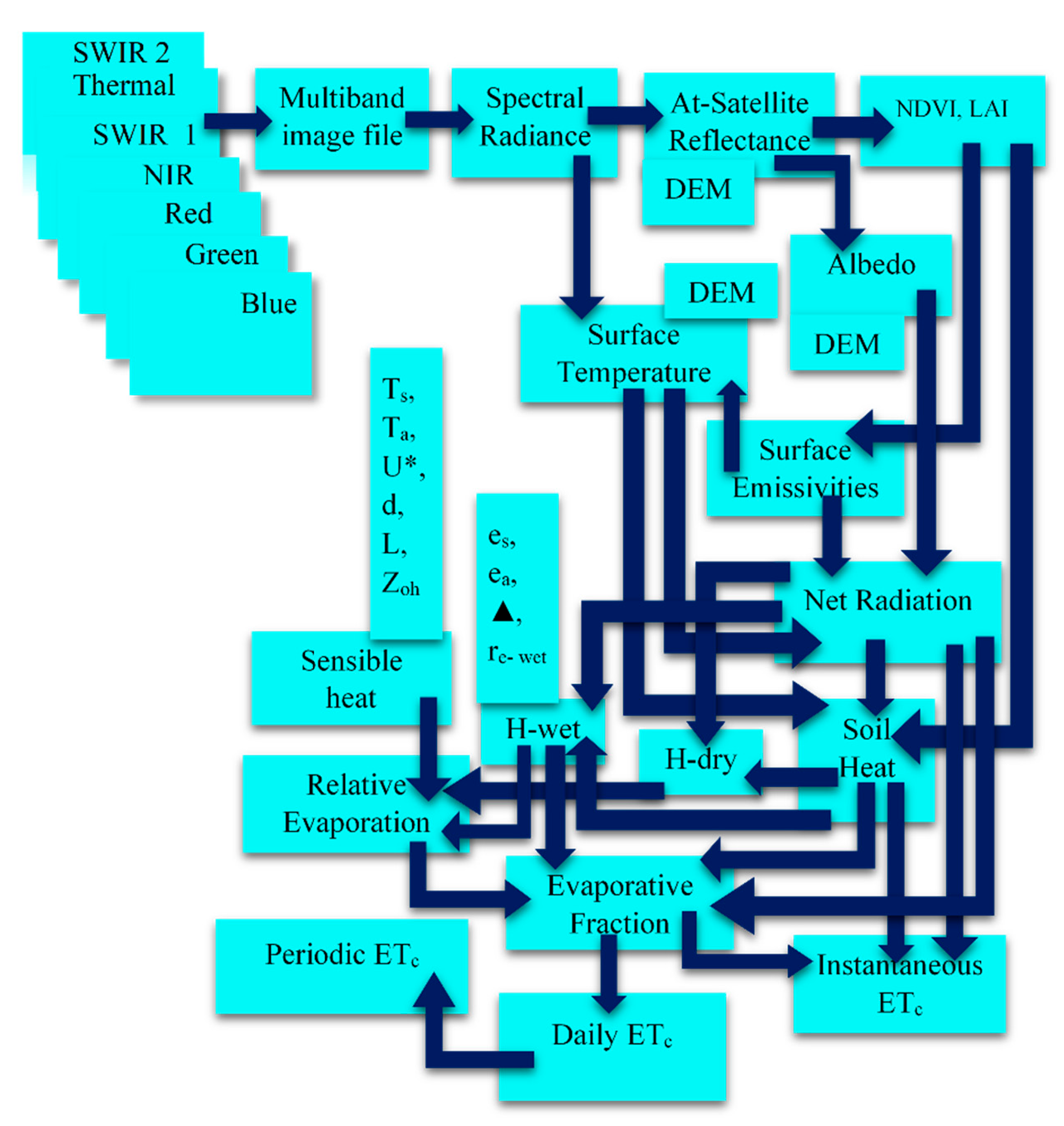
Figure 3.
Flowchart illustrating the computation of surface energy balance fluxes using S-SEBI algorithm.
Figure 3.
Flowchart illustrating the computation of surface energy balance fluxes using S-SEBI algorithm.
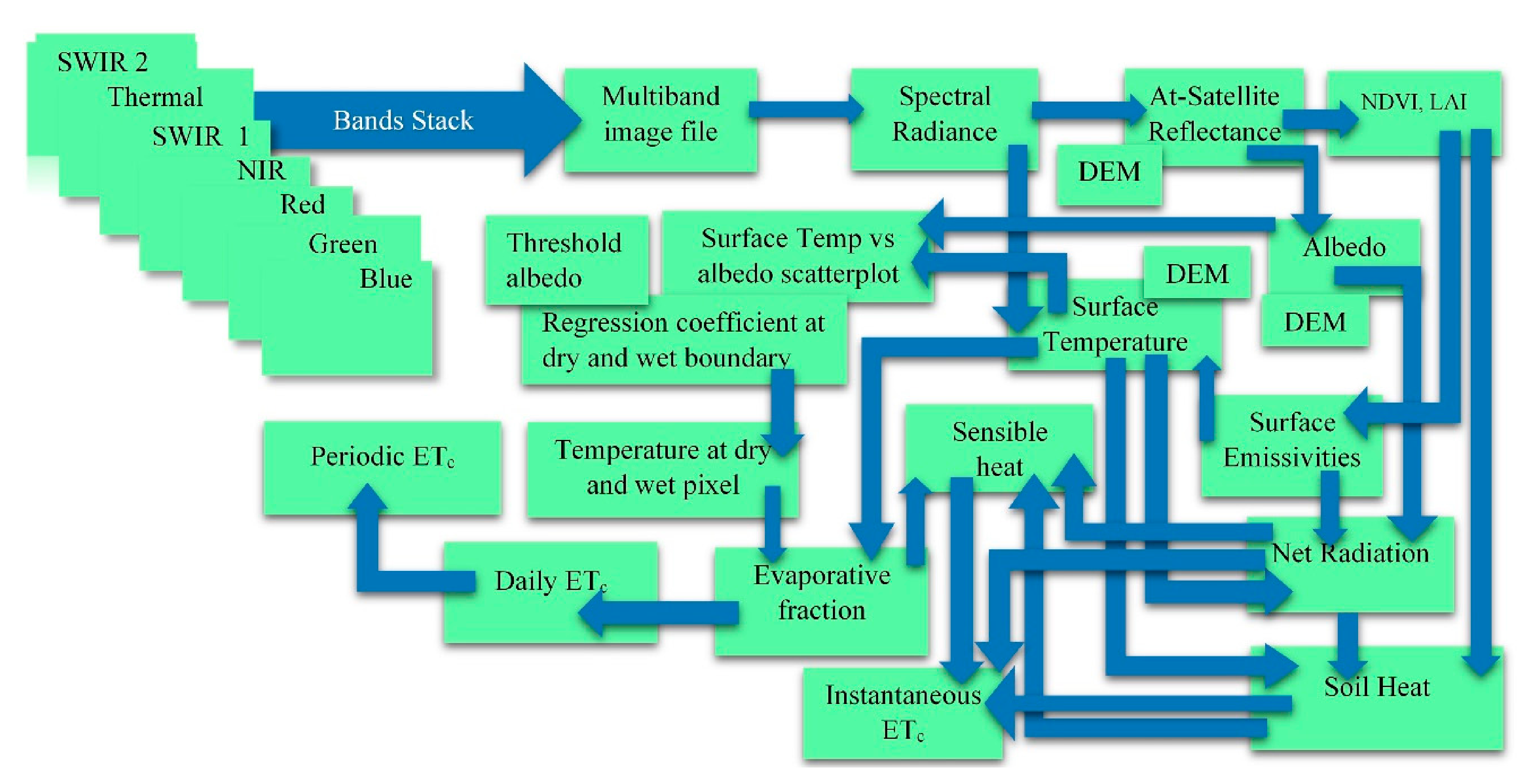
Figure 4.
Scatterplot of Surface albedo and surface temperature (Ts) for Landsat path/row 37/29 on 2 July 2018.
Figure 4.
Scatterplot of Surface albedo and surface temperature (Ts) for Landsat path/row 37/29 on 2 July 2018.

Figure 5.
A comparison of surface energy balance (SEB) model-estimated ETinst (mm h−1) (a) METRIC, (b) SEBAL, (c) SEBS, and (d) S-SEBI with BREBS-measured ETinst at the BREBS flux-tower footprint located in PREC, Powell, Wyoming for three vegetative surfaces.
Figure 5.
A comparison of surface energy balance (SEB) model-estimated ETinst (mm h−1) (a) METRIC, (b) SEBAL, (c) SEBS, and (d) S-SEBI with BREBS-measured ETinst at the BREBS flux-tower footprint located in PREC, Powell, Wyoming for three vegetative surfaces.
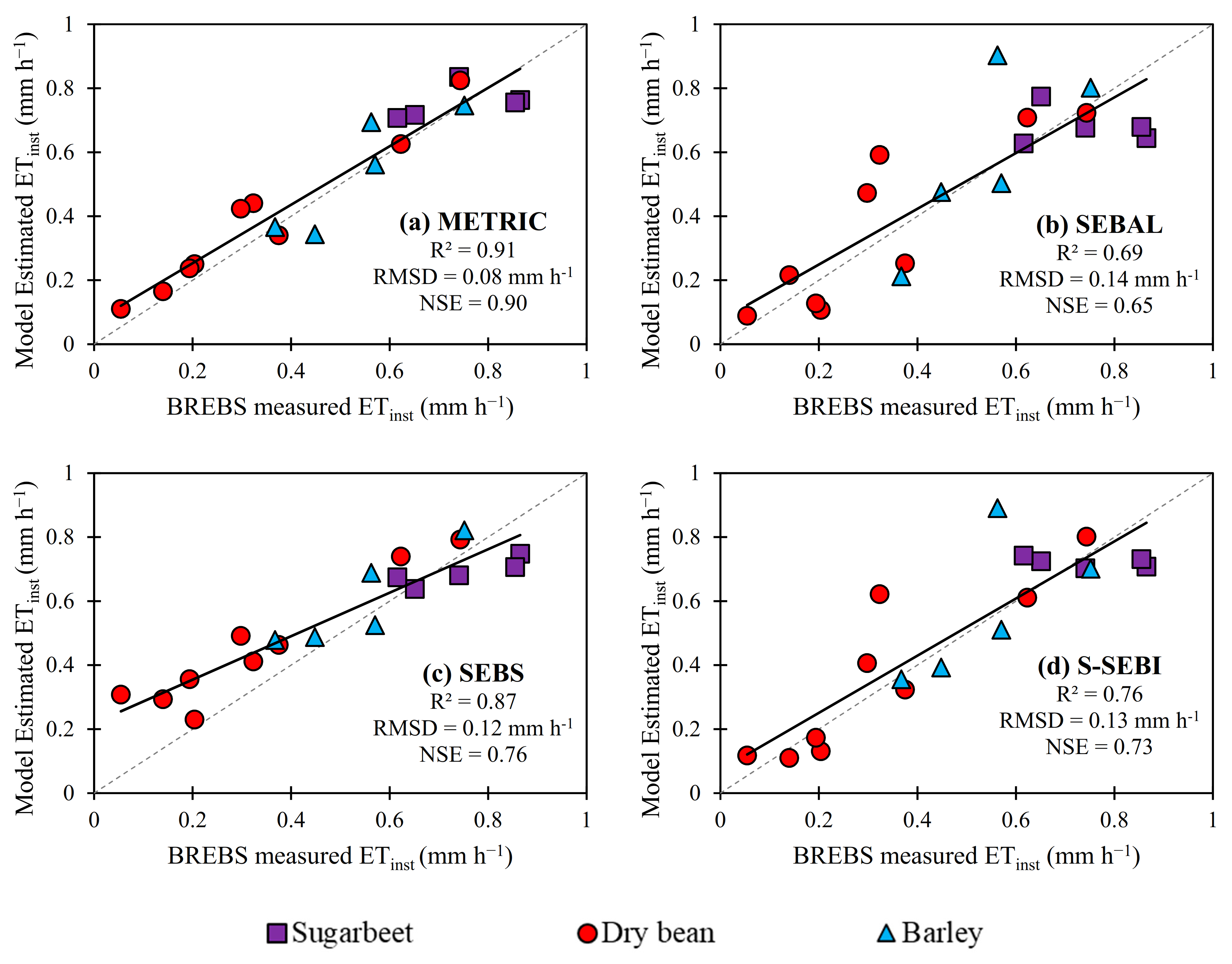
Figure 6.
A comparison of surface energy balance (SEB) model-estimated H flux (W m−2) (a) METRIC, (b) SEBAL, (c) SEBS, and (d) S-SEBI with BREBS-measured H at the BREBS flux-tower footprint located in PREC, Powell, Wyoming for three vegetative surfaces.
Figure 6.
A comparison of surface energy balance (SEB) model-estimated H flux (W m−2) (a) METRIC, (b) SEBAL, (c) SEBS, and (d) S-SEBI with BREBS-measured H at the BREBS flux-tower footprint located in PREC, Powell, Wyoming for three vegetative surfaces.

Figure 7.
Comparison of the model-estimated and BREBS station measured monthly ETc (mm) during 2018 growing seasons.
Figure 7.
Comparison of the model-estimated and BREBS station measured monthly ETc (mm) during 2018 growing seasons.

Figure 8.
Density plot of SEB model estimated ET24 (mm d−1) on: (a) 15 May 2018; (b) 8 June 2018; (c) 2 July 2018; (d) 18 July 2018; (e) 26 July 2018; (f) 11 August 2018; (g) 4 September 2018, and (h) 12 September 2018. (Embedded within each density plot is the mean and mode of ET24 for the corresponding model).
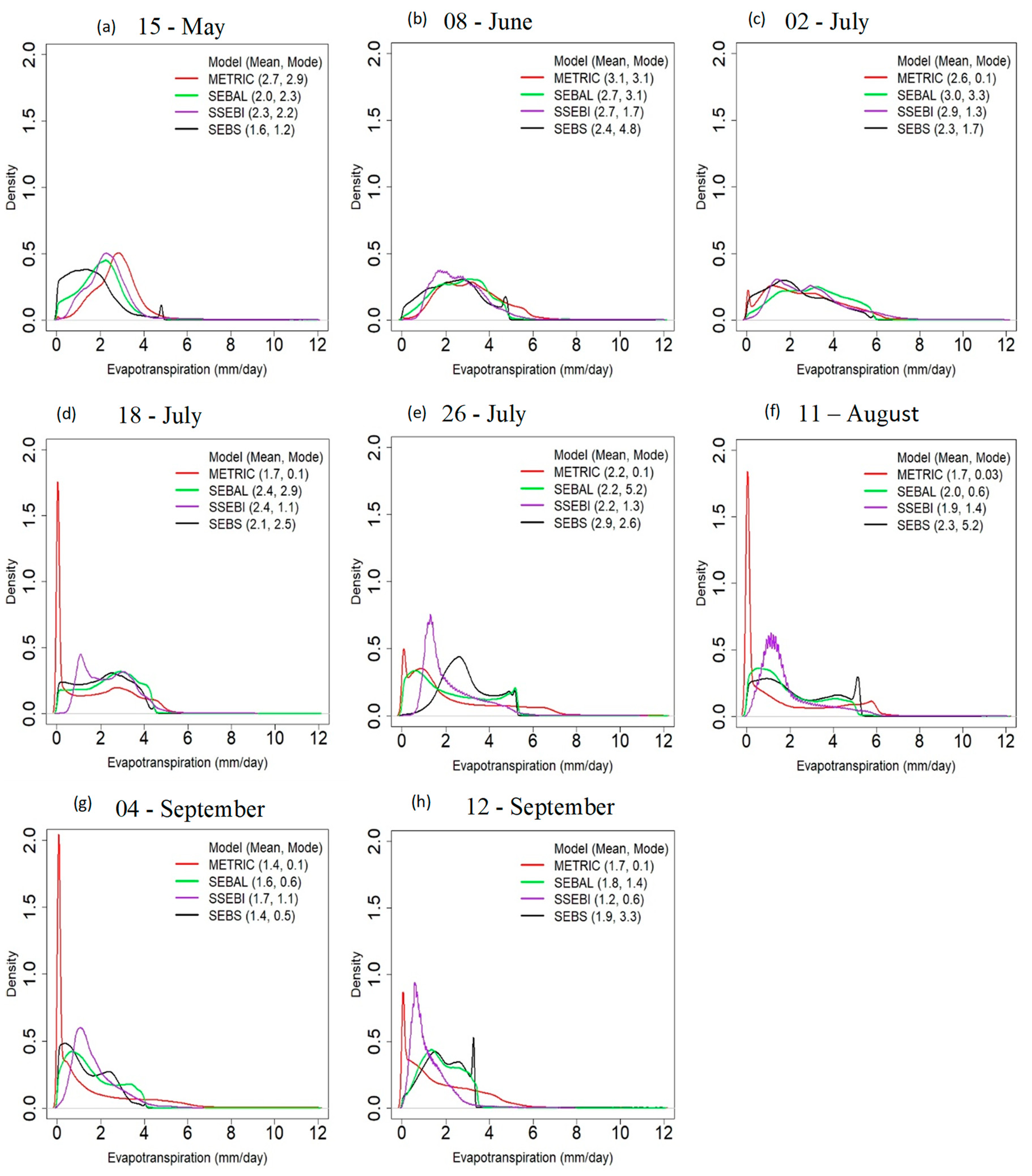
Figure 9.
Density plot comparison of ET24 (mm d−1) between (a) METRIC vs. SEBAL; (b) METRIC vs. SSEBI; (c) METRIC vs. SEBS; (d) SEBAL vs. SSEBI; (e) SEBAL vs. SEBS; (f) SSEBI vs. SEB for 2 July 2018 at image spatial scale.
Figure 9.
Density plot comparison of ET24 (mm d−1) between (a) METRIC vs. SEBAL; (b) METRIC vs. SSEBI; (c) METRIC vs. SEBS; (d) SEBAL vs. SSEBI; (e) SEBAL vs. SEBS; (f) SSEBI vs. SEB for 2 July 2018 at image spatial scale.
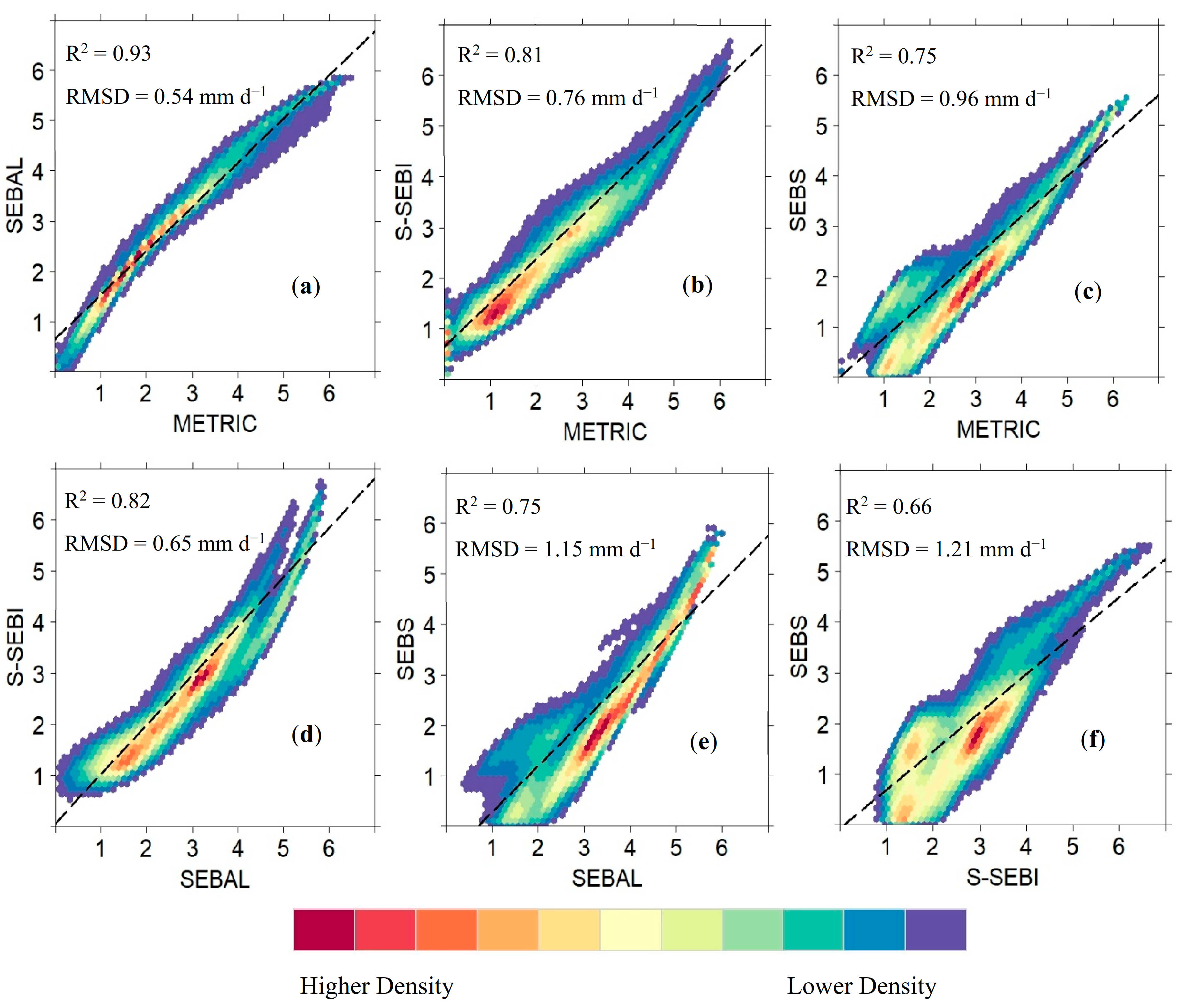
Figure 10.
Absolute difference map between ET24 on 2 July 2018 estimated using different energy balance models: (a) METRIC-SEBAL; (b) METRIC-S-SEBI; (c) METRIC-SEBS; (d) SEBAL-S-SEBI; (e) SEBAL-SEBS; (f) S-SEBI-SEBS.
Figure 10.
Absolute difference map between ET24 on 2 July 2018 estimated using different energy balance models: (a) METRIC-SEBAL; (b) METRIC-S-SEBI; (c) METRIC-SEBS; (d) SEBAL-S-SEBI; (e) SEBAL-SEBS; (f) S-SEBI-SEBS.

Figure 11.
Spatial distribution of SEB model-estimated ET24 on 11 August 2018 (a) METRIC, (b) SEBAL, (c) SEBS, (d) S-SEBI.
Figure 11.
Spatial distribution of SEB model-estimated ET24 on 11 August 2018 (a) METRIC, (b) SEBAL, (c) SEBS, (d) S-SEBI.
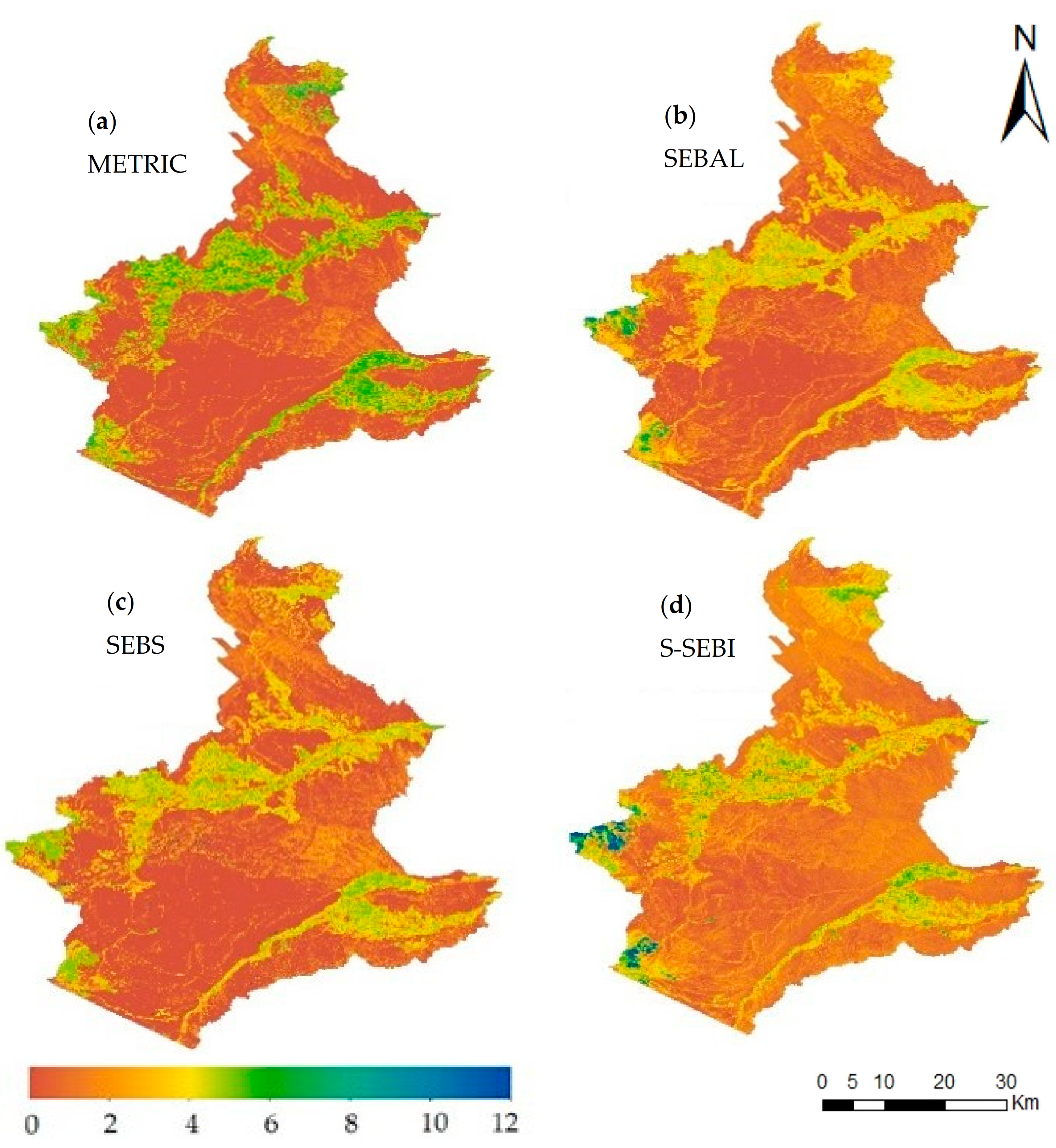
Figure 12.
Spatio-temporal distribution of SEB model-estimated seasonal ETc (mm) across the study area during 2018 growing season (May-September) (a) METRIC, (b) S-SEBI, (c) SEBAL, and (d) SEBS.
Figure 12.
Spatio-temporal distribution of SEB model-estimated seasonal ETc (mm) across the study area during 2018 growing season (May-September) (a) METRIC, (b) S-SEBI, (c) SEBAL, and (d) SEBS.
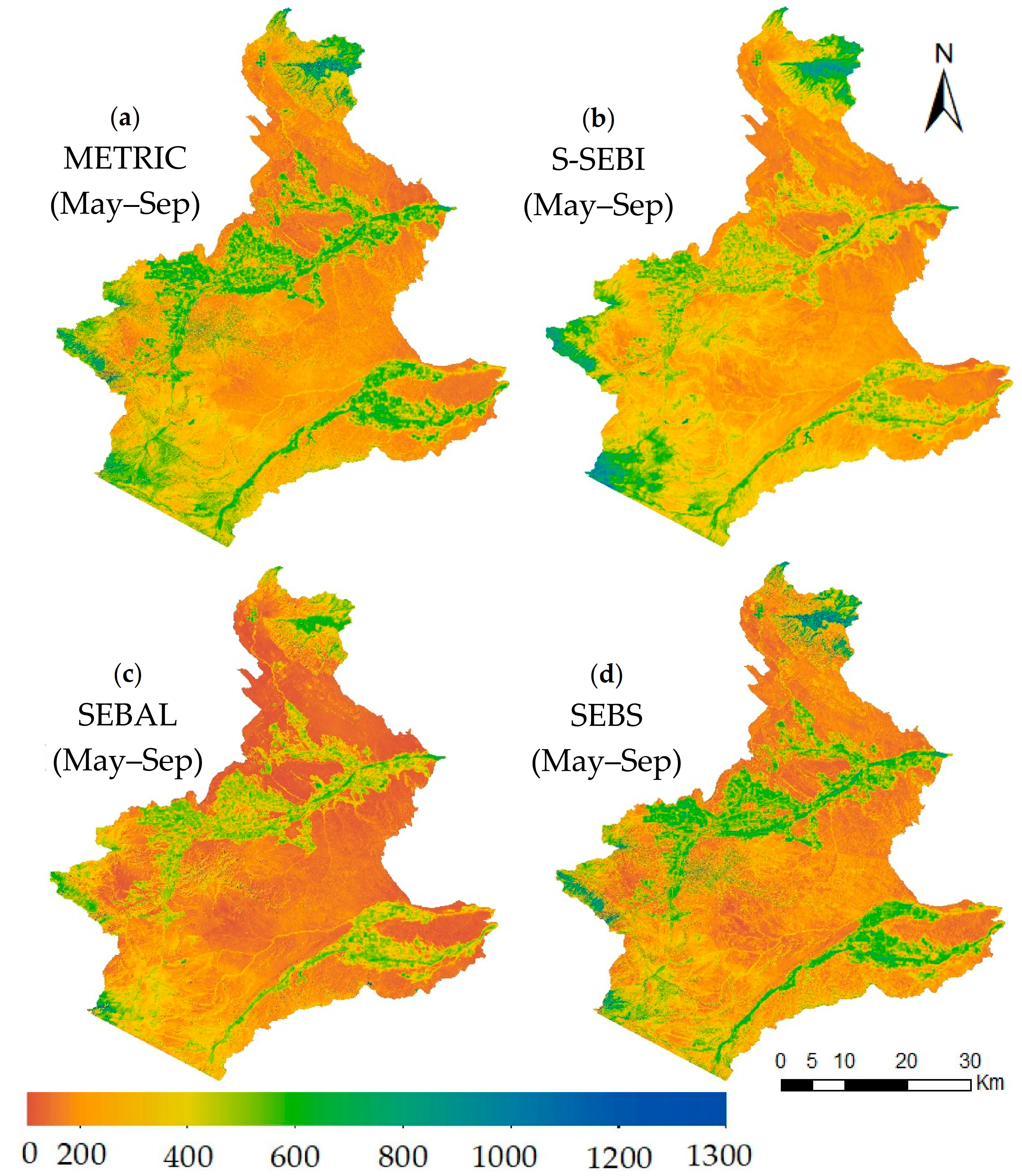

Table 1.
Image acquisition date, spacecraft ID, and daily weather parameters measured at BREBS station, Powell Research and Extension Center, Wyoming. Daily weather parameters include minimum air temperature (Tmin), maximum air temperature (Tmax), minimum maximum air temperature (Tmax), minimum relative humidity (RHmin), maximum relative humidity (RHmax), wind speed (u2), solar radiation (Rs), precipitation (P), and ASCE PM alfalfa-ETr.
| Date | ID | Julian Date | Tmin (°C) | Tmax (°C) | RHmin (%) | RHmax (%) | u2 (ms−1) | Rs (W m−2) | P (mm) | ETr (mm d−1) |
|---|---|---|---|---|---|---|---|---|---|---|
| 15/7/2017 | L08 | 196 | 15.9 | 36.8 | 13.0 | 66.2 | 1.2 | 280.1 | 0 | 7.28 |
| 31/7/2017 | L08 | 212 | 10.8 | 33.3 | 12.4 | 84.3 | 0.9 | 306.0 | 0 | 6.3 |
| 16/8/2017 | L08 | 228 | 9.7 | 25.3 | 22.6 | 82.6 | 0.8 | 217.8 | 0 | 4.14 |
| 1/9/2017 | L08 | 244 | 15.0 | 31.4 | 17.6 | 68.4 | 1.2 | 178.3 | 0 | 5.15 |
| 9/9/2017 | L07 | 252 | 8.1 | 30.2 | 11.6 | 65.6 | 0.8 | 198.2 | 0 | 4.25 |
| 15/5/2018 | L08 | 135 | 6.2 | 19.9 | 33.8 | 100 | 1.4 | 235.9 | 0 | 4.33 |
| 8/6/2018 | L07 | 159 | 10.7 | 27.0 | 24.6 | 82.1 | 1.4 | 230.4 | 0 | 5.55 |
| 2/7/2018 | L08 | 183 | 10.4 | 27.8 | 16.2 | 81.7 | 0.8 | 300.0 | 0 | 5.55 |
| 18/7/2018 | L08 | 199 | 11.8 | 29.5 | 23.6 | 84.0 | 0.7 | 210.6 | 0.254 | 4.55 |
| 26/7/2018 | L07 | 207 | 14.6 | 28.8 | 26.8 | 69.6 | 1.5 | 262.7 | 0 | 6.36 |
| 11/8/2018 | L07 | 223 | 12.4 | 36.4 | 9.0 | 68.2 | 0.7 | 302.5 | 0 | 5.95 |
| 4/9/2018 | L08 | 247 | 6.8 | 30.7 | 11.6 | 77.8 | 1.3 | 261.8 | 0 | 6.03 |
| 12/9/2018 | L07 | 255 | 8.7 | 24.7 | 18.1 | 69.6 | 1.0 | 207.3 | 0 | 4.12 |
| 22/10/2018 | L08 | 295 | −0.2 | 21.6 | 16.8 | 74.0 | 0.9 | 151.5 | 0 | 2.49 |
| 3/6/2019 | L08 | 154 | 8.9 | 27.3 | 20.3 | 84.4 | 1.1 | 301.2 | 0 | 5.97 |
| 13/7/2019 | L07 | 194 | 13.3 | 33.4 | 20.8 | 82.5 | 0.9 | 300.5 | 0 | 6.26 |
| 21/7/2019 | L08 | 202 | 12.0 | 27.5 | 21.8 | 57 | 1.9 | 332.8 | 0 | 7.63 |
| 14/8/2019 | L07 | 226 | 9.5 | 28.3 | 19.4 | 77.8 | 1.2 | 298.5 | 0 | 6.01 |
| 15/9/2019 | L07 | 258 | 8.6 | 29.1 | 13.9 | 80.7 | 1.9 | 192.3 | 0 | 5.99 |
Table 2.
A table describing how various datasets were acquired/ computed in the study.
| Datasets | Models | Source/ Computation |
|---|---|---|
| Landsat 7- ETM+ and Landsat 8- OLI and TIRS | All | USGS (https://earthexplorer.usgs.gov/)(accessed on 6 March 2019) |
| Land use map | All | USDA National Agriculture statistical service (NASS) |
| Digital Elevation Model (DEM) | All | USDA Geospatial Data Gateway |
| Leaf Area Index (LAI) | All | Bastiaanssen [14] empirical equation |
| NDVI and SAVI | All | Using red and near-infrared bands (Huete et al. [45], Huete [46]) |
| Albedo (α) | METRIC and SEBS | Integrating the at-surface band reflectance using weighting coefficients (Starks et al. [47]; Tasumi et al. [48]; Olmedo et al. [49]) |
| SEBAL and S-SEBI | Morse et al. [50] | |
| Surface Temperature (Ts) | All | Modified Planks equation |
| Solar Incidence angle | All | Duffie and Beckman [51] |
| ETr | All | Wyoming Agricultural Climate Network (WACNet; Sharma et al. [42]) |
Table 3.
Statistical comparison between model-estimated and BREBS-measured ETinst for 2017, 2018, and 2019 growing season period.
Table 3.
Statistical comparison between model-estimated and BREBS-measured ETinst for 2017, 2018, and 2019 growing season period.
| MODEL | Year | Surface | N | R2 | Average | Average | SD | SD | PBE | RMSD | NSE |
|---|---|---|---|---|---|---|---|---|---|---|---|
| BREBS flux | MODEL flux | BREBS | MODEL | (mm h−1) | |||||||
| (mm h−1) | (mm h−1) | ||||||||||
| METRIC | 2017 | Sugar beet | 5 | 0.21 | 0.75 | 0.76 | 0.1 | 0.05 | 1.40% | 0.09 | 0.20 |
| 2018 | Dry Bean | 9 | 0.95 | 0.33 | 0.38 | 0.21 | 0.22 | 15.80% | 0.07 | 0.90 | |
| 2019 | Barley | 5 | 0.80 | 0.54 | 0.54 | 0.13 | 0.16 | 0.40% | 0.08 | 0.67 | |
| Pooled data points | 19 | 0.91 | 0.49 | 0.52 | 0.24 | 0.23 | 5.70% | 0.08 | 0.90 | ||
| SEBAL | 2017 | Sugar beet | 5 | 0.06 | 0.75 | 0.68 | 0.1 | 0.05 | −8.70% | 0.14 | −0.90 |
| 2018 | Dry Bean | 9 | 0.75 | 0.33 | 0.37 | 0.21 | 0.25 | 11.40% | 0.13 | 0.64 | |
| 2019 | Barley | 5 | 0.61 | 0.54 | 0.58 | 0.13 | 0.25 | 7.30% | 0.17 | −0.75 | |
| Pooled data points | 19 | 0.69 | 0.49 | 0.5 | 0.24 | 0.25 | 2.20% | 0.14 | 0.65 | ||
| SEBS | 2017 | Sugar beet | 5 | 0.71 | 0.75 | 0.69 | 0.1 | 0.04 | −7.50% | 0.09 | 0.19 |
| 2018 | Dry Bean | 9 | 0.90 | 0.33 | 0.45 | 0.21 | 0.18 | 38.30% | 0.14 | 0.53 | |
| 2019 | Barley | 5 | 0.80 | 0.54 | 0.6 | 0.13 | 0.13 | 11.10% | 0.09 | 0.57 | |
| Pooled data points | 19 | 0.87 | 0.49 | 0.55 | 0.24 | 0.18 | 12.30% | 0.11 | 0.76 | ||
| S-SEBI | 2017 | Sugar beet | 5 | 0.21 | 0.75 | 0.72 | 0.1 | 0.01 | −3.20% | 0.11 | −0.21 |
| 2018 | Dry Bean | 9 | 0.81 | 0.33 | 0.37 | 0.21 | 0.24 | 11.50% | 0.11 | 0.71 | |
| 2019 | Barley | 5 | 0.44 | 0.54 | 0.58 | 0.13 | 0.2 | 5.50% | 0.15 | −0.38 | |
| Pooled data points | 19 | 0.76 | 0.49 | 0.51 | 0.24 | 0.25 | 3.90% | 0.13 | 0.73 | ||
Table 4.
SEB model-estimated mean monthly and seasonal ETc (mm) across the study area along with percentage land cover during the 2018 growing season for 16 different land cover types.
Table 4.
SEB model-estimated mean monthly and seasonal ETc (mm) across the study area along with percentage land cover during the 2018 growing season for 16 different land cover types.
| Land Cover (% Area) | Model | May | Jun. | Jul. | Aug. | Sep. | Total | Land Cover (% Area) | Model | May | Jun. | Jul. | Aug. | Sep. | Total |
|---|---|---|---|---|---|---|---|---|---|---|---|---|---|---|---|
| Open Water (0.2%) | METRIC | 92 | 160 | 186 | 125 | 125 | 688 | Sod/grass seed (0.3%) | METRIC | 101 | 132 | 137 | 105 | 88 | 563 |
| S-SEBI | 128 | 176 | 170 | 115 | 97 | 685 | S-SEBI | 87 | 129 | 132 | 88 | 60 | 496 | ||
| SEBAL | 117 | 162 | 163 | 100 | 84 | 627 | SEBAL | 80 | 126 | 125 | 75 | 61 | 466 | ||
| SEBS | 89 | 122 | 136 | 101 | 153 | 601 | SEBS | 70 | 135 | 163 | 96 | 118 | 582 | ||
| Alfalfa (4.1%) | METRIC | 104 | 146 | 145 | 112 | 102 | 609 | Other hay/non alfalfa (1.4%) | METRIC | 98 | 136 | 126 | 89 | 83 | 533 |
| S-SEBI | 83 | 122 | 122 | 87 | 68 | 481 | S-SEBI | 79 | 119 | 112 | 72 | 60 | 443 | ||
| SEBAL | 85 | 131 | 129 | 80 | 70 | 494 | SEBAL | 75 | 125 | 109 | 59 | 57 | 426 | ||
| SEBS | 68 | 136 | 164 | 98 | 131 | 597 | SEBS | 59 | 128 | 147 | 76 | 114 | 525 | ||
| Sugar Beet (0.9%) | METRIC | 86 | 103 | 174 | 141 | 110 | 614 | Woody wetlands (1.3%) | METRIC | 93 | 146 | 157 | 107 | 91 | 594 |
| S-SEBI | 68 | 100 | 145 | 117 | 79 | 510 | S-SEBI | 90 | 140 | 139 | 87 | 70 | 526 | ||
| SEBAL | 70 | 103 | 155 | 107 | 77 | 511 | SEBAL | 79 | 141 | 145 | 75 | 71 | 511 | ||
| SEBS | 75 | 109 | 184 | 128 | 145 | 641 | SEBS | 72 | 147 | 178 | 96 | 126 | 619 | ||
| Dry Bean (0.8%) | METRIC | 73 | 89 | 124 | 123 | 62 | 471 | Herbaceous wetlands (0.3%) | METRIC | 87 | 123 | 127 | 88 | 84 | 508 |
| S-SEBI | 58 | 69 | 101 | 104 | 45 | 377 | S-SEBI | 77 | 117 | 117 | 73 | 65 | 450 | ||
| SEBAL | 57 | 69 | 105 | 91 | 44 | 366 | SEBAL | 64 | 120 | 119 | 60 | 68 | 430 | ||
| SEBS | 64 | 96 | 157 | 116 | 105 | 539 | SEBS | 45 | 112 | 143 | 69 | 110 | 479 | ||
| Maize (0.6%) | METRIC | 72 | 99 | 163 | 139 | 118 | 592 | Fallow/ Idle crop land (0.1%) | METRIC | 82 | 94 | 80 | 61 | 59 | 376 |
| S-SEBI | 56 | 85 | 129 | 109 | 80 | 459 | S-SEBI | 68 | 91 | 87 | 59 | 44 | 350 | ||
| SEBAL | 56 | 89 | 140 | 102 | 80 | 467 | SEBAL | 59 | 92 | 70 | 40 | 43 | 305 | ||
| SEBS | 61 | 103 | 181 | 125 | 149 | 619 | SEBS | 51 | 97 | 117 | 65 | 98 | 428 | ||
| Spring wheat (0.2%) | METRIC | 87 | 167 | 188 | 103 | 63 | 609 | Shrub land (49%) | METRIC | 71 | 76 | 45 | 16 | 27 | 235 |
| S-SEBI | 70 | 145 | 159 | 85 | 48 | 506 | S-SEBI | 72 | 88 | 75 | 37 | 39 | 311 | ||
| SEBAL | 68 | 148 | 162 | 75 | 46 | 499 | SEBAL | 40 | 68 | 43 | 17 | 49 | 217 | ||
| SEBS | 68 | 159 | 205 | 101 | 106 | 639 | SEBS | 28 | 62 | 74 | 19 | 69 | 252 | ||
| Barley (1.3%) | METRIC | 91 | 166 | 171 | 90 | 64 | 581 | Grass Land (11.4%) | METRIC | 76 | 70 | 33 | 16 | 22 | 217 |
| S-SEBI | 72 | 151 | 154 | 78 | 45 | 500 | S-SEBI | 64 | 70 | 56 | 34 | 31 | 255 | ||
| SEBAL | 72 | 152 | 158 | 65 | 46 | 494 | SEBAL | 38 | 46 | 18 | 13 | 38 | 153 | ||
| SEBS | 71 | 165 | 191 | 90 | 109 | 626 | SEBS | 33 | 55 | 64 | 20 | 64 | 236 | ||
| Oats (0.1%) | METRIC | 77 | 127 | 151 | 103 | 87 | 544 | Barren (0.8%) | METRIC | 71 | 55 | 17 | 12 | 18 | 172 |
| S-SEBI | 60 | 109 | 128 | 83 | 61 | 441 | S-SEBI | 68 | 64 | 51 | 35 | 29 | 246 | ||
| SEBAL | 59 | 116 | 131 | 75 | 63 | 443 | SEBAL | 49 | 49 | 12 | 37 | 59 | 206 | ||
| SEBS | 59 | 127 | 175 | 96 | 122 | 578 | SEBS | 37 | 48 | 54 | 20 | 60 | 219 |
Publisher’s Note: MDPI stays neutral with regard to jurisdictional claims in published maps and institutional affiliations. |
© 2021 by the authors. Licensee MDPI, Basel, Switzerland. This article is an open access article distributed under the terms and conditions of the Creative Commons Attribution (CC BY) license (https://creativecommons.org/licenses/by/4.0/).
Share and Cite
MDPI and ACS Style
Acharya, B.; Sharma, V. Comparison of Satellite Driven Surface Energy Balance Models in Estimating Crop Evapotranspiration in Semi-Arid to Arid Inter-Mountain Region. Remote Sens. 2021, 13, 1822. https://doi.org/10.3390/rs13091822
AMA Style
Acharya B, Sharma V. Comparison of Satellite Driven Surface Energy Balance Models in Estimating Crop Evapotranspiration in Semi-Arid to Arid Inter-Mountain Region. Remote Sensing. 2021; 13(9):1822. https://doi.org/10.3390/rs13091822
Chicago/Turabian StyleAcharya, Bibek, and Vivek Sharma. 2021. "Comparison of Satellite Driven Surface Energy Balance Models in Estimating Crop Evapotranspiration in Semi-Arid to Arid Inter-Mountain Region" Remote Sensing 13, no. 9: 1822. https://doi.org/10.3390/rs13091822
Note that from the first issue of 2016, this journal uses article numbers instead of page numbers. See further details here.