High-Quality Pixel Selection Applied for Natural Scenes in GB-SAR Interferometry

Abstract

Phase analysis based on high-quality pixel (HQP) is crucial to ensure the measurement accuracy of ground-based SAR (GB-SAR). The amplitude dispersion (ADI) criterion has been widely applied to identify pixels with high amplitude stability, i.e., permanent scatterers (PSs), which typically are point-wise scatterers such as stones or man-made structures. However, the PS number in natural scenes is few and limits the GB-SAR applications. This paper proposes an improved method to take HQP selection applied for natural scenes in GB-SAR interferometry. In order to increase the spatial density of HQP for phase measurement, three types of HQPs including PS, quasi-permanent scatter (QPS), and distributed scatter (DS), are selected with different criteria. The ADI method is firstly utilized to take PS selection. To select those pixels with high phase stability but moderate amplitude stability, the temporal phase coherence (TPC) is defined. Those pixels with moderate ADI values and high TPC are selected as QPSs. Then the feasibility of the DS technique is explored. To validate the feasibility of the proposed method, 2370 GB-SAR images of a natural slope are processed. Experimental results prove that the HQP number could be significantly increased while slightly sacrificing phase quality.

1. Introduction

Landslide is one of the most frequent and harmful geological hazards all over the world. Its monitoring and early warning plays an important part in disaster prevention and reduction. Surface deformations normally occur before the macro failure of natural and engineered slopes. Deformation measurement is of great significance to forecast and early warn landslide hazards [1,2]. Spaceborne synthetic aperture radar (SAR) is a powerful and effective remote-sensing technique for surveying large areas (km²). Main limitations are due to its long repetition period in the order of several days or weeks [3,4]. Ground-based SAR (GB-SAR) is a good complementary tool of spaceborne SAR suitable for monitoring deformations of small areas (from a single building to a large slope), with the advantages of all-day, all-weather, high-accuracy, and fast image acquisition [5,6].

With two radar images acquired at different times and from the same position, their interferometric phases could be explored to measure deformations based on the differential interferometry technique [7]. Interferometric phase is the most crucial element that determines the accuracy of deformation measurement. However, due to the influence of several decorrelation sources, such as temporal decorrelation, geometric decorrelation, volume decorrelation, and thermal noise, some pixels with low phase quality in an interferogram are not suitable for phase analysis [8]. An adequate pixel selection method to identify high-quality pixels (HQPs) is essential and important for radar interferometry measurement.

A typical selection criterion is the coherence, which is calculated by applying a boxcar window to spatially average two maps belonging to an interferogram. The coherence criterion is suitable for the analysis of natural scenes with distributed scatterers (DSs), but its averaging operation would easily cause low-quality pixels to be selected, and rarely applied in GB-SAR interferometry [9]. The amplitude dispersion index (ADI) criterion is the most classical one to identify pixels with high amplitude stability, i.e., permanent scatterers (PSs) which could keep highly coherent during a long period. PSs typically are point-wise scatterers which are characterized by high reflectivity, such as stones, man-made structures, and outcrops [10]. This method can be well utilized for urban and rocky scenes, if sufficient images (usually no less than 20) are available.

The absence of strong point-wise PSs is the main obstacle for the PS technique to be applied in natural or vegetational scenes. At the present stage, researches on HQP selection are more focused on the spaceborne SAR rather than GB-SAR applications. The DS technique was proposed by Ferretti et al., where DSs usually correspond to debris areas, non-cultivated land with short vegetation, or desert areas [11]. This method needs to identify statistically homogeneous pixels based on the amplitude similarity. Its feasibility should be explored in GB-SAR interferometry. Hooper et al. proposed to use spatial correlation of interferometric phase to find pixels with low phase variance [12,13]. This method demands an iterative spatial filtering to estimate the noise phase of each pixel, and then adopts the temporal coherence to identify those pixels with high phase stability.

This paper focuses on the HQP selection applied for natural scenes in GB-SAR interferometry, and proposes an improved method. Three types of HQPs including PS, QPS (quasi-permanent scatter), and DS, are selected with different criteria. The conventional ADI method which evaluates a pixel’s amplitude stability is firstly utilized to take PS selection. To select those pixels with high phase stability but moderate amplitude stability, the temporal phase coherence (TPC) is defined. Those pixels with moderate ADI values and high TPC are selected as QPSs. Then the feasibility of the DS technique is explored. With the improved method, 2370 GB-SAR images of a natural slope are processed. Experimental results prove that the HQP number could be significantly increased while slightly sacrificing phase quality.

2. High-Quality Pixel

HQPs for natural scenes refer to those scatterers with high phase stability. Based on the PS concept, the idea is to firstly identify those single-point scatterers with moderate amplitude stability and high phase stability, i.e., QPSs. Then the feasibility of the DS technique is explored in GB-SAR interferometry. Although the temporal coherence of those natural scatterers is typically low, the number of pixels sharing the same statistical behavior can be large enough to make it possible for a few of them to exceed the coherence threshold. Together with the PS, QPS, and DS, the spatial density of the HQP utilized for phase analysis could be significantly increased.

2.1. Permanent Scatterer

PSs refer to those point-wise scatterers which are almost not affected by the spatial and temporal decorrelation over a long time period. The ADI criterion is commonly used by analyzing the amplitude series of a pixel and thresholding on the ADI. The ADI $D_{\mathrm{A}}$ of a pixel can be expressed as

$$D_{\mathrm{A}}={\sigma }_{\mathrm{A}}/m_{\mathrm{A}},$$

(1)

where ${\sigma }_{\mathrm{A}}$ and $m_{\mathrm{A}}$ are the standard deviation and mean value of a pixel’s amplitude series, respectively.

A same numerical simulation with the published research is repeated to show the ADI criterion [10]. For a deterministic point-wise scatterer, its signal model is built as $z_k=g+n_k$$\left(k=1,\cdots ,K\right)$, where g is a pixel’s reflectivity. To better analyze the relationship between the dispersion index $D_{\mathrm{A}}$ and the phase standard deviation ${\sigma }_V$, g is fixed to 1. n is the noise term, and tends to be a complex circular Gaussian distribution with power ${\sigma }_n^2$ for both real and imaginary components. The deviation ${\sigma }_n$ gradually increases from 0.05 to 0.8. For each value of ${\sigma }_n$, 5000 estimates of the ADI values of the amplitude series $A=\left|z\right|$ are completed. Thirty $\left(K=30\right)$ data are supposed to be available.

The mean values (solid line) and the dispersion (error bars) of the estimated ${\widehat{D}}_A$ are shown in Figure 1a, together with the values of the phase standard deviation (dotted line) ${\sigma }_{\mathrm{V}}$. It can be noted that the ADI $D_{\mathrm{A}}$ is a good measure of the phase stability for pixels with high SNR (signal-to-noise ratio). Those pixels exhibiting $D_{\mathrm{A}}$ value under a given threshold $D_{\mathrm{T}}$ (typically lower than 0.25) can be selected as PSs.

Figure 1b shows the scatter map of the dispersion index $D_{\mathrm{A}}$ with the phase std ${\sigma }_{\mathrm{V}}$. For points located under the red line of $D_{\mathrm{A}}=0.25$, their phase std ${\sigma }_{\mathrm{V}}$ varies from 0.05 rad to 0.33 rad (95% confidence interval). Since the ADI is a criterion in a statistical sense, some PSs with relatively large phase std ${\sigma }_{\mathrm{V}}>0.25$ are inevitably selected, as shown with the cyan points in the set ${\mathrm{S}}_2$. Those brown points in the set ${\mathrm{S}}_1$ with $D_{\mathrm{A}}\le 0.25$ and ${\sigma }_{\mathrm{V}}\le 0.25$ are ‘true’ PSs which are stable in both amplitude and phase.

For rocky scenes with lots of deterministic point-wise scatterers, the ‘true’ PS number in the Set ${\mathrm{S}}_1$ is enough for phase analysis. Therefore, based on the ADI criterion, another phase criterion could be further utilized together to reduce and refine the set ${\mathrm{S}}_1{+\mathrm{S}}_2$ to ${\mathrm{S}}_1$. However, for natural scenes, even if only the ADI criterion is utilized, the PS number in ${\mathrm{S}}_1{+\mathrm{S}}_2$ is still few. To increase the point number suitable for differential interferometry, those points with moderate amplitude stability and high phase stability, as shown with the yellow points in the set ${\mathrm{S}}_3$, could be utilized. This type of point is defined as QPS.

2.2. Quasi-Permanent Scatterer

QPS refers to a pixel with moderate amplitude stability and high phase stability, i.e., a moderate ADI $D_{\mathrm{A}}$ and a small phase std ${\sigma }_{\mathrm{V}}$. The interferometric phase ${\phi }_{\mathrm{Int}}$ of a pixel in GB-SAR interferometry could be modeled as:

$${\phi }_{\mathrm{Int}}= \mathrm{W}\left[{\phi }_{\mathrm{defo}}+{\phi }_{\mathrm{atm}}+{\phi }_{\mathrm{geom}}+{\phi }_{\mathrm{noi}}\right],$$

(2)

where ${\phi }_{\mathrm{defo}}$ is the deformation phase component, ${\phi }_{\mathrm{atm}}$ is the phase component due to the atmospheric effects during image acquisitions, ${\phi }_{\mathrm{geom}}$ is a geometrical phase term due to the aperture variation or repositioning error. ${\phi }_{\mathrm{noi}}$ is the noise term. $\mathrm{W}[ ]$ denotes the phase wrapped function.

In order to evaluate the phase stability of a pixel, the TPC ${\gamma }_{\mathrm{TPC}}$ is defined [14]. $N_{\mathrm{IN}}$ denotes the interferogram number, or the length of a pixel’s phase sequence. The value range of ${\gamma }_{\mathrm{TPC}}$ is from 0 to 1, and a larger value means a better stability of ${\phi }_{\mathrm{noi}}$. A key problem is how to accurately estimate the noise term from the interferometric phase. The basic solution is to design a filtering framework based on the different temporal and spatial properties of those four phase terms in (2).

$${\gamma }_{\mathrm{TPC}}=\left|{\displaystyle \sum _{n=1}^{N_{\mathrm{IN}}}\exp \left(j{\phi }_{\mathrm{noi}}^{\left(n\right)}\right)}\right|/N_{\mathrm{IN}},$$

(3)

A further analysis of the numerical simulation in the Section 2.1 is made. Take interferometry process for each data sequence, and the interferometric phase ${\phi }_{\mathrm{Int}}$ of any two neighboring data can be regarded as the noise phase ${\phi }_{\mathrm{noi}}$. Based on (3), the TPC ${\gamma }_{\mathrm{TPC}}$ of each point is calculated. The mean values (solid line) and the dispersion (error bars) of ${\gamma }_{\mathrm{TPC}}$, together with the values of the phase std ${\sigma }_{\mathrm{V}}$ (dotted line), are shown in Figure 2a. Contrast with Figure 1a, ${\gamma }_{\mathrm{TPC}}$ decreases with the increasement of the noise std ${\sigma }_n$. Figure 2b shows the scatter map of the TPC ${\gamma }_{\mathrm{TPC}}$ with the phase std ${\sigma }_{\mathrm{V}}$. For those pixels with phase std ${\sigma }_{\mathrm{V}}$ lower than 0.25 rad, i.e., left part of the green dotted line, 99.99% of them are with the TPC ${\gamma }_{\mathrm{TPC}}$ larger than 0.91. To some extent, the TPC ${\gamma }_{\mathrm{TPC}}$ is an equivalent criterion with the ADI $D_{\mathrm{A}}$.

To better illuminate the relationship between the TPC ${\gamma }_{\mathrm{TPC}}$ and the ADI $D_{\mathrm{A}}$, Figure 3a shows the scatter map of ${\gamma }_{\mathrm{TPC}}$ with $D_{\mathrm{A}}$. By setting two proper thresholds of ${\gamma }_{\mathrm{T}}$ and $D_{\mathrm{T}}$, those pixels with ${\gamma }_{\mathrm{TPC}}\ge {\gamma }_{\mathrm{T}}$ and $D_{\mathrm{A}}>D_{\mathrm{T}}$ in the set ${\mathrm{S}}_3$ could be selected as QPSs. For those pixels with the ADI $D_{\mathrm{A}}$ lower than 0.25, and belonging to S₁ + S₂, their TPC values are between 0.91 and 0.99 (90% confidence interval). The mean values (solid line) and the dispersion (error bars) of ${\gamma }_{\mathrm{TPC}}$ with $D_{\mathrm{A}}$, are shown in Figure 3b. When $D_{\mathrm{A}}$ equals to 0.25, the variation range of ${\gamma }_{\mathrm{TPC}}$ is about from 0.91 to 0.96. Moreover, for those pixels with the TPC ${\gamma }_{\mathrm{TPC}}$ larger than 0.91, and belonging to the set S₁ + S₃, 99.99% of them are with the ADI $D_{\mathrm{A}}$ lower than 0.45. Therefore, those pixels with the TPC ${\gamma }_{\mathrm{TPC}}$ larger than 0.91, but with the ADI $D_{\mathrm{A}}$ between 0.25 and 0.45, could be selected the QPSs.

2.3. Distributed Scatterer

DSs refer to those scatterers which are affected by temporal, geometrical, and volumetric decorrelation, but their phase quality could be improved with their neighboring homogeneous pixels [15].

Ferretti et al. proposed an algorithm named by DespecKS to identify a pair of statistically homogeneous pixels [11]. To evaluate whether two pixels $P_1$ and $P_2$ are homogeneous, the two-sample KS test is utilized. By measuring the maximum difference $D_K$ between the cumulative probability distribution functions $S_K^{P_1}\left(x\right)$ and $S_K^{P_2}\left(x\right)$ of their amplitude sequences, two pixels are homogeneous if $D_K$ is lower than a proper threshold.

$$D_K=\sqrt{K/2}\sup \left|S_K^{P_1}\left(x\right)-S_K^{P_2}\left(x\right)\right|, S_K\left(x\right)=\{\begin{array}{l}0\hspace{1em}\hspace{1em}\hspace{1em}if x<x_i\\ i/K\hspace{1em} if x_i\le x<x_{i+1}\\ 1\hspace{1em}\hspace{1em}\hspace{1em}if x\ge x_K\end{array}$$

(4)

where K is the sequence length, and $x_1,x_2,\dots ,x_K$ is the sorted amplitude sequence of a pixel. Figure 4a shows two curves whose amplitudes randomly vary and cannot determine their similarity. Figure 4b shows their sorted amplitude curves. With KS test, both curves satisfy the same normal distribution, and they can be regarded as a pair of homogeneous pixels.

Take an image-pixel P as an example, and then define an estimation window centered on P. Apply two-sample KS test to count the number of its homogeneous pixels. Setting a proper number threshold, P can be regarded as a DS if its homogeneous pixels are enough. For a DS, its phase quality could be enhanced with its surrounding homogeneous pixels. It should be noted that only those DSs whose phase qualities are good enough could be utilized for phase analysis, and a further optimization is essential.

3. Pixel Selection

To select enough HQP for natural scenes, the key problem is how to accurately select QPS, and explore the feasibility of DS selection in GB-SAR interferometry.

3.1. PS Selection

Given $N$ (no less than 20) GB-SAR images, two different ADI thresholds $D_{\mathrm{T}1}$ (0.1 to 0.25) and $D_{\mathrm{T}2}$ (0.25 to 0.45) are firstly utilized to take initial selection. With a small ADI threshold to select PS, the possibility of those PSs with large phase errors could be reduced effectively. Pixels with ADI value $D_{\mathrm{A}}\le D_{\mathrm{T}1}$ are set as the reference PSs. Pixels with ADI value $D_{\mathrm{T}1}<D_{\mathrm{A}}\le D_{\mathrm{T}2}$ are set as the candidate set of the QPS (${\mathrm{CS}}_{\mathrm{QPS}}$). Based on those reference PSs, the candidate set should be refined.

3.2. QPS Selection

With N GB-SAR images, every two consecutive images could be explored to construct an interferogram. Then the length of a pixel’s interferometric phase sequence, or the interferogram number is $N_{\mathrm{IN}}=N-1$. To calculate a pixel’s TPC, the noise phase ${\phi }_{\mathrm{noi}}$ in (2) should be estimated. The first three terms ${\phi }_{\mathrm{defo}}$, ${\phi }_{\mathrm{atm}}$, and ${\phi }_{\mathrm{geom}}$ in (2) are highly spatially correlated, while ${\phi }_{\mathrm{noi}}$ is spatially uncorrelated. Therefore, a spatial filter could be utilized to filter out the spatial phase components and estimate ${\phi }_{\mathrm{noi}}$.

The reference PSs distribute non-uniformly on the interferogram. They can be divided into a certain number of clusters according to their spatial locations with a K-means clustering algorithm, which is a method commonly utilized to automatically partition a point set into K clusters [16]. As shown in Figure 5, those scatter points are partitioned into 5 clusters which are marked with different colors. The sign ‘x’ denotes each cluster center.

For those PSs belonging to a same cluster, calculate their mean location $\overline{r}$ and mean phase ${\overline{\phi }}_{\mathrm{Clu}}^{}$. Since the interferometric phase ${\phi }_{\mathrm{Int}}$ of each pixel is wrapped, the circular period mean filter is utilized, as shown below.

$$\begin{array}{l}{\overline{\phi }}_{\mathrm{Clu}}^{}={\displaystyle \sum _{i=1}^{N^{\mathrm{Clu}}}\arg \left[\exp \left(j{\phi }_{\mathrm{Int}}^{\mathrm{Clu}\left(i\right)}\right)/d_{\mathrm{Clu}}\right]}/N^{\mathrm{Clu}}+\arg \left(d_{\mathrm{Clu}}\right)\\ d_{\mathrm{Clu}}={\displaystyle \sum _{i=1}^{N^{\mathrm{Clu}}}\exp \left(j{\phi }_{\mathrm{Int}}^{\mathrm{Clu}\left(i\right)}\right)}/N^{\mathrm{Clu}}\end{array}$$

(5)

For a cluster, $N^{\mathrm{Clu}}$ is the total pixel number belonging to it, and ${\phi }_{\mathrm{Int}}^{\mathrm{Clu}\left(i\right)}$ denotes the interferometric phase of its ith pixel. $d_{\mathrm{Clu}}$ is the mean value of the complex phase of all the pixels belonging to this cluster. $\arg [ ]$ is the function to get the phase angle of a complex value.

For every pixel belonging to ${\mathrm{CS}}_{\mathrm{QPS}}$, its spatial phase component ${\phi }_{\mathrm{Spa}}$ should be estimated. A 2-D spatial interpolation could be utilized, such as linear or Kriging interpolation. It should be noted that the complex phase $\exp (j{\overline{\phi }}_{\mathrm{Clu}})$ rather than the wrapped phase ${\overline{\phi }}_{\mathrm{Clu}}$ should be used for interpolation. Subtracting ${\phi }_{\mathrm{Spa}}$ from ${\phi }_{\mathrm{Int}}$, the residual phase is ${\phi }_{\mathrm{noi}}$ [17].

This method is commonly utilized to compensate the space-variant phase in GB-SAR interferometry, if only those montionless PSs with no deformations are used for K-means cluster. Research has proved that the geometrical term ${\phi }_{\mathrm{geom}}$ caused by repeat-track error in GB-SAR interferometry could be similarly modeled with the atmospheric phase. Undoubtedly, ${\phi }_{\mathrm{geom}}$ can be well compensated with the interpolation method. Although the deformation term ${\phi }_{\mathrm{defo}}$ cannot be compensated thoroughly, its residual component during a short period for a slow-moving scene could be neglected.

Based on (3), the TPC of a pixel could be estimated with (6). ${\phi }_{\mathrm{Int}}^{\left(n\right)}$ is the nth value of a pixel’s interferometric phase sequence. ${\phi }_{\mathrm{Spa}}^{\left(n\right)}$ is its estimated spatial phase component.

$${\gamma }_{\mathrm{TPC}}=\left|{\displaystyle \sum _{n=1}^{N_{\mathrm{IN}}}\exp \left(j{\phi }_{\mathrm{Int}}^{\left(n\right)}-j{\phi }_{\mathrm{Spa}}^{\left(n\right)}\right)}\right|/N_{\mathrm{IN}},$$

(6)

Setting a proper TPC threshold ${\gamma }_{\mathrm{T}}$, those pixels with ${\gamma }_{\mathrm{TPC}}$ no smaller than ${\gamma }_{\mathrm{T}}$ are selected as QPSs. Other pixels with ${\gamma }_{\mathrm{TPC}}$ smaller than ${\gamma }_{\mathrm{T}}$ are then selected to be the candidate set of the DS (${\mathrm{CS}}_{\mathrm{DS}}$).

3.3. DS Selection

For a pixel belonging to ${\mathrm{CS}}_{\mathrm{DS}}$, it is used as a window center, and then determined its homogeneous pixel according to whether their amplitude curves satisfy a same distribution. If the number of its homogeneous pixels is large enough, it can be selected as a DS. The key problem is how to improve the phase quality of these DSs, since their coherence is low and cannot be directly utilized for phase analysis.

The coherence matrix $\mathbf{\Gamma }\left(P\right)$ of a DS P could be estimated as,

$$\mathbf{\Gamma }\left(P\right)=\mathrm{E}\left[d\left(P_{\Omega }\right)d^H\left(P_{\Omega }\right)\right]\approx \frac{1}{N_{\mathrm{HP}}}{\displaystyle \sum _{P\in \Omega }d\left(P_{\Omega }\right)d^H\left(P_{\Omega }\right)},$$

(7)

where $\mathbf{\Omega }$ is the homogeneous pixel set of a DS $P$, and $N_{\mathrm{HP}}$ denotes the number of its homogeneous pixels. $d=\exp \left(j\mathsf{\phi }\right)$ is the complex vector of a pixel belonging to $\mathbf{\Omega }$, and $\mathsf{\phi }={\left[{\phi }_1, {\phi }_2, \cdots , {\phi }_N\right]}^H$ is its phase vector. ${}^H$ denotes the complex conjugate.

Based on the coherence matrix $\mathbf{\Gamma }\left(P\right)$, a method of maximum likelihood estimation could be utilized to extract the optimal phase $\mathsf{\lambda }={\left[{\vartheta }_1, {\vartheta }_2,\cdots ,{\vartheta }_N\right]}^T$ of the DS $P$, as shown in (7). $\mathsf{\Lambda }$ is a column vector and equals to $\exp \left(j\lambda \right)$. $·$ denotes the Hadamard product. A newton iteration method can be used to solve this optimization problem.

$$\widehat{\lambda }=\mathrm{argmax}\left\{{\mathsf{\Lambda }}^H\left({\left|\Gamma \right|}^{-1}·\mathsf{\Gamma }\right)\mathsf{\Lambda }\right\},$$

(8)

Once the optimal solution $\mathsf{\lambda }$ has been obtained, the quality of the estimated phase values ${\vartheta }_i$ should be assessed. Another type of coherence ${\gamma }_{\mathrm{DS}}$ could be utilized to be a ‘goodness of fit’ measure. Select every DS with ${\gamma }_{\mathrm{DS}}$ higher than the TPC threshold ${\gamma }_{\mathrm{T}}$, and then substitute the original phase values with its optimized values.

$${\gamma }_{\mathrm{DS}}=\frac{1}{N^2-N}{\displaystyle \sum _{n=1}^N{\displaystyle \sum _{k\ne n}^N\exp \left[j\left({\vartheta }_n-{\vartheta }_k\right)\right]\exp \left[-j\left({\phi }_n-{\phi }_k\right)\right]}},$$

(9)

3.4. HQP Selection

The processing flow developed for the HQP selection is shown in Figure 6, and it can be presented schematically as follows:

(1)

Two different ADI thresholds $D_{\mathrm{T}1}$ and $D_{\mathrm{T}2}$ are utilized for initial selection. Pixels with ADI value $D_{\mathrm{A}}\le D_{\mathrm{T}1}$ are set as the reference PSs. Pixels with $D_{\mathrm{T}1}<D_{\mathrm{A}}\le D_{\mathrm{T}2}$ are set as ${\mathrm{CS}}_{\mathrm{QPS}}$.

(2)

Based on the K-means clustering and spatial filtering, ${\gamma }_{\mathrm{TPC}}$ of every pixel belonging to ${\mathrm{CS}}_{\mathrm{QPS}}$ is calculated. Setting a proper ${\gamma }_{\mathrm{T}}$, those pixels with ${\gamma }_{\mathrm{TPC}}$ no smaller than ${\gamma }_{\mathrm{T}}$ are selected as QPSs, and other pixels belong to ${\mathrm{CS}}_{\mathrm{DS}}$.

(3)

For every pixel belonging to ${\mathrm{CS}}_{\mathrm{DS}}$, its homogeneous pixels are determined. Define those pixels whose homogeneous pixels are enough as DSs. For each DS, phase optimization with its homogeneous pixels is made. Those DSs with coherence ${\gamma }_{\mathrm{DS}}$ large than ${\gamma }_{\mathrm{T}}$ are reserved.

(4)

Together with the PS, QPS, and DS as the HQP, the traditional PSInSAR algorithm could be utilized for differential interferometry.

4. Experimental Information

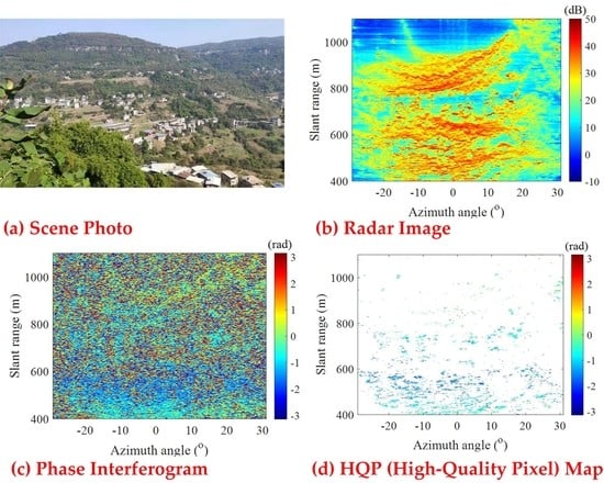
From 10:39 on 20 April 2019 to 8:08 on 30 April 2019 (China Standard Time), a GB-SAR system was utilized to monitor a vegetational scene (N30°50′39.83″, E108°25′3.58″) located in Wanzhou district, Chongqing City, China. The plane form of this slope is a chair-like shape, as shown in Figure 7. The slope is about 80 m to 108 m long, 120 m to 250 m wide, with an average thickness of 13.33 m, and a volume of about 298,000 m³. It is a typical medium-scale middle-layer soil landslide. A village is located at the slope foot and on the slope. Those residential buildings are strong scatterers, i.e., PSs in the GB-SAR images.

Figure 8 shows the photo of the GB-SAR. The instrument was developed by Beijing Institute of Technology, and provided by Suzhou Institute of Technology Reco Sensing Technology Co., Ltd. As a developed type of high-accuracy deformation measurement system, GB-SAR has been widely utilized to monitor surface deformations of natural or geological slopes.

Table 1. Parameters of the GB-SAR system.

Parameter	Value
central frequency	16.2 GHz
wavelength	1.85 cm
synthetic aperture	1.8 m
bandwidth	600 MHz
resolution	0.25 m × 5 mrad @1 km
measuring range	50 m to 5 km

show the system parameters. The system works at Ku band with a wavelength of 1.85 cm. The transmitted signal is a frequency-modulated continuous wave. With the transmitting and receiving antennas moving along a high-precision mechanical track, a large aperture of 1.8 m could be synthesized. For a GB-SAR system with a fixed-length track, the Ku-band wave is conducive to a significant improvement in its azimuth resolution. In addition, it benefits increasing the measurement accuracy under the condition of a same level of noise phase, contrast with a lower-band wave. Although the Ku-band electromagnetic wave cannot penetrate vegetations, those bare soils or ground surfaces make it feasible to select QPS and DS [8].

The experiment lasted for about 10 days, a total of 2370 images were acquired during the monitoring period. The average image acquisition time was about 6 min. Figure 9a shows a power image of the monitoring area at the polar coordinate, which was dB processed with respect to the average noise level, and could be regarded as a signal-to-noise ratio (SNR) map. Take the first $N=30$ images as an example. Based on (1), the ADI value of every pixel could be calculated with these $N$ amplitude images. Figure 9b shows the ADI map. Pixels with ADI values lower than 0.25 only occupy about 2.3%.

With the 1st image as the master image, and the 2nd and 30th images as the slave images, two interferograms ${\mathrm{IM}}_{1–2}$ and ${\mathrm{IM}}_{1–30}$ could be acquired. Figure 10a shows the phase interferogram ${\mathrm{IM}}_{1–2}$, whose temporal baseline is just several minutes. As a result of the atmospheric disturbance, for pixels located on the natural slope, their phases vary smoothly. The atmospheric refractivity affects the propagation speed of the radar wave through the troposphere. Different transmission delays could be inevitably caused due to the variant atmospheric condition, and it could even reach centimeter level at one kilometer. Atmospheric phase is one major error source in GB-SAR measurement, and must be well compensated [18]. Figure 10b shows the interferogram ${\mathrm{IM}}_{1–30}$, whose temporal baseline reaches about three hours. Its phase variation is much more noisy in contrast with that of ${\mathrm{IM}}_{1–2}$, since this vegetational scene is affected by the temporal decorrelation over a time period of several hours.

5. Experimental Results

For the first 30 images acquired from 10:40 to 13:34 on 20 April 2019 (China Standard Time), by setting an ADI threshold of $D_{\mathrm{T}1}=0.25$, 25,575 reference PSs could be selected. Figure 11a shows the phase map of the reference PSs based on the interferogram ${\mathrm{IM}}_{1–2}$, which sparsely distribute on the whole map. By setting an ADI threshold of $D_{\mathrm{T}2}=0.45$, 159,753 pixels with ADI values $D_{\mathrm{T}1}<D_{\mathrm{A}}\le D_{\mathrm{T}2}$ are selected, and they belong to the set ${\mathrm{CS}}_{\mathrm{QPS}}$. Figure 11b shows the phase map of these pixels, which distribute on most parts of the whole map. A regular phase variation caused by the atmospheric disturbance can be observed. In addition, lots of noisy pixels exist, since the threshold $D_{\mathrm{T}2}$ is larger than the typical threshold $D_{\mathrm{T}1}$ utilized for PS selection. This phenomenon illuminates the feasibility of further selecting pixels with high phase quality.

These reference PSs are divided into 70 clusters, as shown in Figure 12a. Those black squares denote the cluster centers, and every polygon marks the boundary of every cluster. With an inverse distance weighting interpolation, the spatial phase components of the pixels belonging to ${\mathrm{CS}}_{\mathrm{QPS}}$ are estimated, as shown in Figure 12b. It is worth noting that the estimated phases vary regularly both along the range and azimuth direction. For the phase components along the range direction, they are caused by the atmospheric disturbance at different times. While for the components along the azimuth direction, published researches prove that they are caused by the repeat-track error when radar moves along the mechanical track [19].

After compensating the spatial phase components, the TPC of those pixels belonging to ${\mathrm{CS}}_{\mathrm{QPS}}$ is calculated based on (6), as shown in Figure 13a. According to the analysis conclusion in Section 2.2, a TPC threshold of ${\gamma }_{\mathrm{T}}=0.91$ equivalent to the ADI threshold of $D_{\mathrm{T}}=0.25$ is set. A total number of 20,364 QPSs can be selected, as shown in Figure 13b. Contrast with the PS number, the QPS number occupies about 79.6%. Pixels with the TPC ${\gamma }_{\mathrm{TPC}}$ lower than the threshold ${\gamma }_{\mathrm{T}}=0.91$ belong to the set ${\mathrm{CS}}_{\mathrm{DS}}$. Figure 13c shows the probability density curves of ${\gamma }_{\mathrm{TPC}}$ of the reference PSs and ${\mathrm{CS}}_{\mathrm{QPS}}$. The shapes of both curves are much different. This illuminates that with a lower ADI threshold, pixels with high amplitude stability are more possible to be also with high phase stability. Figure 13d shows the scatter map of ${\gamma }_{\mathrm{TPC}}$ with $D_{\mathrm{A}}$ for the reference PSs and ${\mathrm{CS}}_{\mathrm{QPS}}$. Its distribution trend is much similar with the simulation results shown in Figure 3a. The PS number belonging to the set ${\mathrm{S}}_2$, i.e., ${\gamma }_{\mathrm{TPC}}<0.91$ and $D_{\mathrm{A}}\le 0.25$, is 2251 and makes up 8.8%. Although the phase quality of this type of PSs is doubtful, there is low necessity to further refine them for the natural scenes. The QPS belonging to the set ${\mathrm{S}}_3$ makes up about 12.75% of the set ${\mathrm{CS}}_{\mathrm{QPS}}$. Therefore, for pixels with high ADI values, it is rather hard to squeeze out enough pixels with high phase stability.

After the QPS selection, the remaining pixels are belonging to the set ${\mathrm{CS}}_{\mathrm{DS}}$. For every pixel, it is used as the center of a 5 × 7 rectangular window, where 5 is the pixel number along the azimuth direction, and $7$ is along the range number. The statistically homogeneous pixel of every pixel is determined based on the two-sample KS test. Figure 14a shows the homogeneous pixel map of ${\mathrm{CS}}_{\mathrm{DS}}$. By setting a number threshold of $N_{\mathrm{T}}=10$, 111,406 DSs could be selected. Based on (7)–(9), ${\gamma }_{\mathrm{DS}}$ of these DSs are calculated and shown in Figure 14b. With the coherence threshold ${\gamma }_{\mathrm{T}}=0.91$, 4260 DSs are reserved. Although the DS number is only 16.7% of the PS number, it still benefits increasing the pixel number utilized for differential interferometry. Figure 14c shows the phase map of the selected DSs, which sparsely distribute on the map. Above all, a total of 50,199 HQPs are selected, including 25,575 PSs, 20,364 QPSs, and 4260 DSs. Figure 14d shows the phase map of the HQPs. Contrast with the PSs selected only with the ADI criterion, the HQPs increase by 96.3%. The spatial density of the pixels for deformation analysis has been significantly increased. Other than the increase in the HQP number, analysis on the phase quality should be further made.

For the first 30 images, 29 interferograms ${\mathrm{IM}}_{1–2}$, ${\mathrm{IM}}_{2–3}$, …, and ${\mathrm{IM}}_{29–30}$ could be formed by every two consecutive images. Based on the PS-InSAR algorithm, these interferograms are processed, including phase unwrapping, atmospheric compensation, and deformation measurement. Figure 15a shows the cumulative deformation map. Since these images were acquired during three hours, it was impossible for this slow-moving landslide to displace for several millimeters. Then the standard deviation of every HQP’s deformation is calculated, and utilized to quantitively evaluate the phase quality of the PSs, QPSs, and DSs. Figure 15b shows the probability density curves of these three types of pixels. Most of the PSs are with deformation deviations around 0.3 mm, while for most of the QPSs and DSs, their deformation deviations are both around 0.42 mm. It is possibly caused by that a relatively low coherence threshold of ${\gamma }_{\mathrm{T}}=0.91$ is utilized, compared with the ADI threshold of $D_{\mathrm{T}1}=0.25$.

Every $N=30$ images of all the 2370 images are divided into an image group. For each group, the HQP selection is taken with the same processing for the 1st group. Figure 16a shows the number curves of different types of HQPs for all the 79 groups. It should be noted that the number fluctuations of PS, QPS, and DS for time-series image groups are normal phenomena in GB-SAR applications, which is mainly caused by daily temperature variation, and could be solved by an adaptive selection threshold [7]. The PS numbers of different image groups change between 6355 and 46,920, and its average number is 17,702. In addition, the average numbers of QPS and DS are 10,052 and 3389, and their increase ratios contrast with the average PS number are 56.8% and 19.1%, respectively. Therefore, with the improved method to select the QPS and DS, the HQP number could be significantly increased. For the 12th image group, its HQP number is the most, and reaches 78,935, as shown in Figure 16b. The HQP density is much larger than that of the 1st group.

It is worth noting that the DS numbers in these groups are no more than 6958, and the average DS number is only 19.1% of PS. However, the procedures to take DS selection include homogeneous pixel calculation, phase optimization, and coherence thresholding, which need much computation. Although the DS technique in GB-SAR interferometry is feasible, the DS density is rather small. A lower coherence threshold could be set to select more DSs, but larger deformation deviations are unavoidable. Therefore, the necessity of DS selection in GB-SAR applications is low, unless when the PS number is rather few for a natural slope.

Figure 17 shows the cumulative deformation map during the monitoring period of 10 days. Since the monitored slope is a creep landslide, no large deformation area is found during a relatively short period, but some pixels with measurement errors of several mm are unavoidable. No other instruments with deformation measurement ability were available for the creep slope during the monitoring period. Only qualitative explanations can be made to illustrate the effectiveness of the improved method.

6. Discussion

Pixels with high phase equality are essential and important for radar interferometry measurement. A common method is based on the ADI criterion to select PSs, as shown in Figure 1, which typically refer to deterministic point-wise scatterers, such as rocks. However, for natural scenes, the absence of point-wise PSs could severely affect interferometry measurement. Aiming at increasing the spatial density of HQP applied for natural scenes, an improved method to jointly select PS, QPS, and DS has been proposed.

With 30 GB-SAR images of a natural slope, 25,575 pixels with the ADI values $D_{\mathrm{A}}$ lower than 0.25 are firstly selected as the PSs, and those pixels with $0.25<D_{\mathrm{A}}\le 0.45$ are selected as ${\mathrm{CS}}_{\mathrm{QPS}}$, as shown in Figure 11. Then based on these PSs, the K-means clustering and spatial interpolation are utilized to calculate the TPC ${\gamma }_{\mathrm{TPC}}$ of every pixel belonging to ${\mathrm{CS}}_{\mathrm{QPS}}$. A total of 20,364 pixels with ${\gamma }_{\mathrm{TPC}}\ge 0.91$ are selected as QPSs, and those pixels with ${\gamma }_{\mathrm{TPC}}<0.91$ are taken as ${\mathrm{CS}}_{\mathrm{DS}}$, as shown in Figure 13. Lastly, the two-sample KS test is utilized to calculate the homogeneous pixels of every pixel belonging to ${\mathrm{CS}}_{\mathrm{DS}}$, and a number threshold is set to select DS. Based on (7) and (8), ${\gamma }_{\mathrm{DS}}$ of every DS is estimated. With a coherence threshold of ${\gamma }_{\mathrm{T}}=0.91$, 4260 DSs are reserved.

To validate the effectiveness of the proposed method, analyses are made from two aspects. As for the 30 images acquired during 3 h, the standard deviation of every HQP’s deformation is calculated. As shown in Figure 15b, most PSs are with deformation deviations around 0.3 mm, while for QPSs and DSs, their deformation deviations are both around 0.42 mm. While slightly sacrificing phase quality, the HQP number has been significantly increased. As for the 2370 images acquired during 10 days, 79 image groups are taken HQP selection. Statistical results in Figure 16a show that the average numbers of PSs, QPSs, and DSs are 17,702, 10,052, and 3389, respectively.

7. Conclusions

This paper proposes an improved method to take HQP selection applied for natural scenes in GB-SAR interferometry. In order to increase the spatial density of HQP for phase measurement, three types of HQPs including PS, QPS, and DS, are selected with different criteria. The conventional ADI method which evaluates a pixel’s amplitude stability is firstly utilized to take PS selection. In order to select those pixels with high phase stability but moderate amplitude stability, a TPC criterion is adopted to take QPS selection. In addition, the feasibility of the DS technique in GB-SAR interferometry is explored. With a GB-SAR system, 2370 images of a natural slope were acquired during an experimental period of 10 days. As for the 30 images acquired during 3 h, statistical results of the deformation deviations prove that the HQP number can be significantly increased, while slightly sacrificing phase quality. As for the 2370 images acquired during 10 days, statistical results of the HQP numbers of 79 groups prove that, contrast with the average PS number, an average increase of 56.8% and 19.1% can be got with the QPS and DS selection.

Although experimental datasets validate the effectiveness of the proposed method, this paper needs more experimental verification. More natural scenes, especially those without residential buildings or bare rocks, should be measured to validate the feasibility to select the HQP. In addition, other measurement techniques, such as GPS, spaceborne SAR, and laser scanner, should be also utilized to measure the same scene, and provide comparative verification with the GB-SAR.