
Joint Ship Detection Based on Time-Frequency Domain and CFAR Methods with HF Radar


1
The School of Electronic Information, Wuhan University, Wuhan 430072, China
2
East China Sea Forecast Center, State Oceanic Administration, Shanghai 200136, China
3
Wuhan Hailanruihai Ocean Technology Co. Ltd., Wuhan 430223, China
*
Author to whom correspondence should be addressed.
Remote Sens. 2021, 13(8), 1548; https://doi.org/10.3390/rs13081548
Submission received: 16 February 2021
/
Revised: 10 April 2021
/
Accepted: 11 April 2021
/
Published: 16 April 2021
(This article belongs to the Special Issue Feature Paper Special Issue on Ocean Remote Sensing)
Abstract
:Compact high-frequency surface wave radar (HFSWR) plays a critical role in ship surveillance. Due to the wide antenna beam-width and low spatial gain, traditional constant false alarm rate (CFAR) detectors often induce a low detection probability. To solve this problem, a joint detection algorithm based on time-frequency (TF) analysis and the CFAR method is proposed in this paper. After the TF ridge extraction, CFAR detection is performed to test each sample of the ridges, and a binary integration is run to determine whether the entire TF ridge is of a ship. To verify the effectiveness of the proposed algorithm, experimental data collected by the Ocean State Monitoring and Analyzing Radar, type SD (OSMAR-SD) were used, with the ship records from an automatic identification system (AIS) used as ground truth data. The processing results showed that the joint TF-CFAR method outperformed CFAR in detecting non-stationary and weak signals and those within the first-order sea clutters, whereas CFAR outperformed TF-CFAR in identifying multiple signals with similar frequencies. Notably, the intersection of the matched detection sets by TF-CFAR and CFAR alone was not immense, which takes up approximately 68% of the matched number by CFAR and 25% of that by TF-CFAR; however, the number in the union detection sets was much (>30%) greater than the result of either method. Therefore, joint detection with TF-CFAR and CFAR can further increase the detection probability and greatly improve detection performance under complicated situations, such as non-stationarity, low signal-to-noise ratio (SNR), and within the first-order sea clutters.
1. Introduction
Maritime surveillance is an important task for coastal nations in coastal conservancy, security, fishery, and managing their exclusive economic zones (EEZs) [1,2] where the location and motion information of the ships are especially valuable. High frequency surface wave radar (HFSWR) uses high frequency (3–30 MHz) vertical polarized electromagnetic wave, which can propagate along this surface with small attenuation, and, thus, has the capability of remote sensing of moving targets at sea. Up to now, there are more than 400 HF radar sites in operation for ocean observation globally. For example, the United States, Europe, Japan, and Australia have built nearly complete HF radar observation networks [3], which provide real-time sea surface state parameters such as current velocity, wind speed, and wave heights. Part of these radar systems have also been used for ship detection. To increase maritime domain awareness, SeaSonde HF radar coastal ocean current and wave-monitoring networks have been used for vessel detection in New York Harbor. In April 2011, real-time vessel detection software was installed and run in parallel with the current mapping software running locally at the radar sites. Since this time, thousands of vessels have been successfully detected entering and exiting the harbor, ranging from smaller pleasure craft (15–20 m) to large shipping vessels (100+ m) [4]. The Wellen Radar (WERA) system [5] finds applications in oceanography and can be used to detect and track ships. A ship detection and tracking algorithm for WERA HF-radar has been developed using three-dimensional (3D) ordered-statistic (OS)-constant false alarm rate (CFAR) algorithm and a scheme similar to the well-known α-β tracker [6]. The effectiveness of this HF-radar as a long range (≈130 km) continuous-time surveillance system is also shown in [7]. Canada’s third-generation HFSWR system [8,9] uses hybrid (CFAR) detectors for ship detection, which can decrease the quantity of false detection in heavy-clutter regions and increase the target detection probabilities in the medium- and low-clutter regions. It also allows use of more advanced tracking techniques so that the system is able to maximize the probability of tracking while minimizing the probability of false alarms or other erroneous tracks. Nikolić et al. used a modified Cell Averaging Greatest of CFAR (CAGO-CFAR) for target detection in range, azimuth, and Doppler [10] with the detection threshold relying on an assumption of Weibull distribution and an averaged signal level, which led to a higher detection probability than CAGO-CFAR. Since a major proportion of radar systems operated all over the world use compact receive antennas, the ship detection performance with compact radar is of interest. Strong sea clutter and interference are two main challenges to ship detection [11], which usually demands a relatively high threshold for constant false alarm rate (CFAR) detection. This problem is even worse for compact radars since the small array aperture means a low spatial gain. Another challenge is the non-stationarity of the ship echoes since a relative long coherent integration time (CIT) is needed to detect such slow targets. Consequently, compact HFSWR usually has a low detection probability (Pd), which is an urgent problem to be solved.
Ship detection is conventionally performed on the range-Doppler (RD) spectrum which is calculated using a two-dimensional (2D) Fourier transform (FT) of the radar signal. The CFAR technique uses an adaptive threshold for automatic signal detection, which is proportional to the mean power of the local clutters. One basic adaptive algorithm is the cell-averaging CFAR (CA-CFAR) method introduced by Finn and Janson [12]. The CA-CFAR detector performs optimally in a uniform distributed clutter, but it will cause an excessive increase in the false alarms at the edge of clutter and a decrease in the detection performance in a multi-target environment. The greatest of (GO) CFAR and smallest of (SO) CFAR were proposed by Hansen and Trunk [13,14] to further solve the problems such as missing targets near the clutter edges due to clutter region expansion and missing small targets under multiple target situations. These conventional CFAR methods can only solve part of the problems, but also bring some extra detection losses. Moreover, they all have a poor performance in the cases of low signal-to-noise ratio (SNR) and non-stationary target.
The characteristics of the moving target in the Doppler frequency domain and the background clutter model [15,16] are two key factors for detection. Clutters or interference whose Doppler spectra are superimposed on the spectral peak of a ship tend to decrease Pd. Meanwhile, because a relatively long CIT is used to detect ships, non-stationarity is also a disadvantage which may spread the signal power onto a series of Doppler bins and, thus, may also lower Pd. The RD spectrum is insufficient to describe the local information, e.g., the duration and the change of the instantaneous frequency (IF) of a signal. If the detailed local characteristics in the time and frequency can be fully used, the moving target can be better recognized with instantaneous details of the target being achieved. Time-frequency analysis (TFA) is such an efficient tool to solve this problem. Thayaparan et al. [17] analyzed the performances of 12 TFA methods for stationary and non-stationary target detection and concluded that the reassigned transforms provide the better signal resolution and have excellent performance in detecting non-stationary targets and, thus, can help better understand and analyze radar signals. Jangal et al. [18] extracted sea clutter based on wavelet decomposition and reconstruction to improve the ability of target detection of HFSWR. The target signal on the RD map was enhanced by at least 20–30 dB after reconstructing the wavelet coefficients, which is very conducive to ship detection, but the weight of the wavelet coefficients is empirical rather than adaptive that needs to be adjusted continuously to obtain a better RD map. Carretero-Moya et al. [19] proposed a target detection method based on Radon transform, but it can only detect targets with high velocities for high-resolution radar, such as millimeter wave radar. Lei and Huang [20] used short-time Fourier transform (STFT) and image processing technology (e.g., the area growth method) to detect maneuvering target ridges with Doppler close to clutter with an over-the-horizon radar (OTHR), but this method has disadvantages of computing-intensiveness and blurry TF ridges by STFT. Grosdidier et al. [21,22] used morphological component analysis (MCA) method to improve target detection of HFSWR, where the separation of sea clutter and target signal can be driven by sparsity when a proper dictionary (transform) is chosen. Compared with classical CFAR techniques, MCA-CFAR shows better results on simulated data of a single target but, unfortunately, its detection performance has not been verified with real radar data. Inspired by Jangal, Lu et al. [23] proposed a vessel detection method based on a compact-array HFSWR system, which uses principle component analysis (PCA) and wavelet decomposition to enhance the RD spectra and suppress clutter, respectively. Compared with Jangal’s method, the SNR of the target can be further improved, but disadvantages are similar because the selection of wavelet coefficients also relies on experience. Focusing on the problems in Jangal’s method, Li et al. [24] presented an automatic ship target detection algorithm based on discrete wavelet transform (DWT). It can automatically select the optimal scale of DWT to separate point targets from background clutters with Ostu algorithm [25], but cannot quantitatively describe the detection probability (Pd) and the false alarm probability (Pfa) of the target, therefore, one cannot decide whether the extracted point targets are real targets or not. To sharpen the TF ridges, Cai et al. [26] used synchro-extracting transform (SET) and image edge detection to extract the TF ridges, which achieved improved detection of moving targets in the broadened and splitting Doppler spectrum. Hao et al. [27] used the combination of SET and short time fractional Fourier transform (SSTFrFT) and calculated the Rényi entropy of the unit where the target is located to detect a single target with an X-band radar. This method can accurately distinguish moving targets from sea clutters, but did not give a statistical analysis of the detection.
The above methods have enhanced the detection ability of non-stationary and weak targets to certain degree, but have not established the corresponding detection and false alarm probability, thus it is difficult to accurately evaluate their performances in specific applications. To this end, in this study, a joint detection method by TF-CFAR and CFAR is proposed to improve the detection probability of the target. In TF ridge detection, the time frequency representation (TFR) is first binarized, and projection along the time axis is performed to determine the coarse frequency range of the ridge according to the average and peak value of the projection. Then, the greedy search algorithm is used to extract the TF ridge in that area, and the binary integration (BI) algorithm is used to determine whether the TF ridge is a target signal. In this process, the CFAR method is involved to determine whether a TF point is a target point and whether a ridge is a target ridge. The advantage of such TF-CFAR processing is that it can lower the detection threshold of CFAR and, thus, more target signals can be recognized without increasing Pfa. Moreover, one major feature of this TF-CFAR processing is the persistence and energy accumulation of the TF ridge, which is particularly useful for detecting non-stationary and weak targets. With the aid of automatic identification system (AIS) information, experimental evaluation of the performances of TF-CFAR methods for ship detection becomes easier than ever. The dataset used here is collected by the broad-beam HF radar named the Ocean State Monitoring and Analyzing Radar, type SD (OSMAR-SD) [28] working at 13.15 MHz. Compared with the conventional CFAR detection, the method proposed in this study has advantages in the number of target detection and the detection of non-stationary targets, weak targets, and targets within the first-order peak.
The remaining of this paper is organized as follows. Section 2 describes the probability distribution model of the sea clutter for the CFAR method. Section 3 presents the TF-CFAR detection method and describes the TF ridge extraction and detection. Experimental evaluation of the joint processing results is described in Section 4. Section 5 gives some discussions. Section 6 gives a brief conclusion.
2. Conventional CFAR Method
2.1. Signal Model and Sea Clutter Probability Distribution
For slow targets such as ships, the movements are often within one range bin, e.g., 2.5 km in this study, so we have the following expression for a maneuvering target at a certain range bin:
where A(t) is the instantaneous amplitude, φ(t) is the instantaneous phase, and fd(t) = 2v(t)/λ with v(t) being the instantaneous velocity and λ the wavelength. The detection model in a clutter background can be expressed as:
where t is time and c(t) denotes the clutter. CFAR detection is usually performed on the power spectrum or amplitude spectrum. Barrick once reported in 1977 [29] that the real and imaginary components of the HF radar echo from the sea surface were approximately Gaussian distributed, the amplitude envelope was Rayleigh distributed, and the power was exponential distributed. However, it was later found that the RD spectrum can be better described with a two-parameter Weibull distribution [30], whose probability density distribution function (PDF) is given by:
where x is clutter amplitude, b is the scale parameter, and c denotes the shape parameter. The Weibull distribution reduces to the Rayleigh and exponential distributions when c = 2 and 1, respectively, so the Weibull distribution is a more general distribution. Before the detection, the unknown parameters should be estimated by fitting the experimental data. For example, the sea clutter PDF model obtained with real radar data on 25 September 2015 is shown in Figure 1.
Figure 1 is achieved using 44,318 samples of the background sea clutter taken from the radar spectra between the positive and negative first-order peaks at the 60th range bin on 25 September 2015. The significant wave height at this time was about 0.5 m. By fitting to the Weibull distribution, the estimated scale parameter is b = 282.05 and the shape factor is c = 1.76. The calculated PDF of the clutter and the fitted model of the Rayleigh distribution are also shown in Figure 1. It can be seen that the sea clutter data fit the Weibull distribution well and much better than the Rayleigh distribution. The model parameters may change under different sea states, which should thus be estimated before the processing begins. Notably, any linear transform of the sea clutter also follows a Weibull PDF model. In this study, linear TFR is involved, which uses a synchrosqueezing transform (SST) based on short-time Fourier transform (STFT) [31]. Therefore, the sea clutter in the TF domain also follows the Weibull distribution model.
2.2. CA-CFAR
In the CA-CFAR detector, the background clutter power level Z is estimated by the average value of N = 2n samples of the reference units. The structure of the CA-CFAR detector is shown in Figure 2.
The relationship between Pfa−CA, and the normalization factor T in the CA-CFAR method is [32,33]
where Γ(·) denotes the gamma function, T is the nominal factor dependent on Pfa−CA, and c is the shape parameter of PDF estimated by the sea clutter. The parameter of c needs to be known in advance when calculating T, mainly because the shape parameter will change under different sea states. Under low and high sea state, c will slightly increase and decrease respectively. The product of T and Z constructs the CA-CFAR decision threshold S. If the cell under test is greater than or equal to S, the decision will be H1, otherwise the decision will be H0.
3. Joint Detection Method
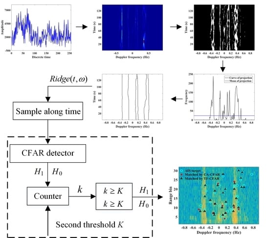
The TF-BI algorithm and CA-CFAR detection technologies are jointly used for ship detection in this study. SST is used to convert the time series on each range bin into a 2D TFR, which mostly considers the evolutionary details of the signal. CA-CFAR detection is performed on the RD spectrum, which helps control the false alarm rate of the detection. Figure 3 shows the block diagram of the joint detector.
3.1. TFR and Binarization
SST is a postprocessing method with frequency reassignment based on the TFR, whose main idea is to sharpen the TF ridges by increasing the TF energy concentration through squeezing the signal spectral components with an identical instantaneous frequency (IF) [34,35]. SST has been widely used in different fields due to its high TF concentration and easy implementation.
Assume that the radar target satisfies a single-component signal model described by Equation (1). The STFT of signal s(t), which is used to calculate the TFR, is given by:
where g(τ − t) denotes the moving window. For any (t, ω) when STFT(t, ω) ≠ 0, the IF estimate can be obtained by:
where denotes the derivative operator with respect to time and ω is circular frequency. STFT has advantages of low computational cost and no cross terms between signal components, but its TF ridge is blurry, which may critically affect the final detection capability. Fortunately, this problem can be solved by SST. It has been proven that [36,37] setting and assuming being sufficiently small, for , we have the approximation:
where is the first-order derivative of the signal phase with respect to time. Equation (7) shows that for a slowly time-varying signal, the IF estimate can sufficiently approach the true IF. SST uses a frequency reassignment operator to gather the spread TF coefficients, which is given by:
where denotes the estimate of ω and is the Kronecker delta function. By SST, the blurry energy of the STFT around the IF trajectories of each signal component is squeezed so that a TFR much concentrated than STFT can be obtained, which is useful for subsequent ship detection.
Figure 4 shows the TFR and the binarization processing of the radar signal. Figure 4a,b are the power spectrum and TFR of the radar echo signal at the 7th range bin, respectively. Figure 4c is the binarized image of Figure 4b. Figure 4b–d are corresponding to the preprocessing of Figure 3. It can be seen that, after the binarization, the ridges with a longer duration and big energy or some strong noises are retained as target pixels (see Figure 4c). However, after the binarized image is accumulated and projected along the time axis, the strong noise points are generally lower than the average value of the projection curve (see Figure 4d), which is equivalent to filtering before the TF ridge extraction and, thus, helps to reduce false alarms. Then, the range of Doppler frequency for TF ridge extraction is determined according to the peak and mean values of the projection curve (see Figure 4d). That is, the regions where the projection curve exceeds the mean value are considered as of target TF ridges, which corresponds to Fl in Equation (9). If a region of TF ridge has less than three Doppler bins, it will be discarded because it is more like noise. Meanwhile, the zero-Doppler region is excluded from the detection.
After the binarization processing, the binary grayscale image is projected along the time axis. Then the area for TF ridge extraction is determined according to the peak and average values of the projection curve (see Figure 4d). TF ridges in different areas are extracted, which can be expressed as [38]:
where l is the index of the TF ridge extraction area, Fl is the set of frequency bins at the l-th TF ridge extraction area, Ridgel(t) denotes the obtained ridge curve, and here M = 256. After a TF ridge is extracted, the TF ridge is sampled with an equal interval to obtain the test unit:
where i = (p − 1)∆T + 1 for p = 1, …, 16 with ∆T = 16. The CA-CFAR detector is used for each sample to determine whether it is a target.
3.2. Binary Integration Method
After CA-CFAR is used for the first level of detection, the second level of detection uses BI detection. When one detection unit is recognized, a protection unit and three reference units are provided on both sides of the detection unit, and then the BI method is used to further determine the number of target points. If the number of the first-level target points reaches a preset threshold, the area is considered the target area, and the TF ridge extracted from the area is considered a target. The theoretical solutions of the BI method [39,40] are given below.
The probabilities, say Pfa and Pd, of the BI detection are related to a group of samples along Ridge(ti). Then, the relationship between Pfa and Pd as well as the Pfa,sp and Pfa,d of a single observation is established. For the BI detection, the following two assumptions are usually made.
- D1 ≥ S1, D2 ≥ S2, ···, Dm ≥ Sm, i.e., these events are independent.
- Pfa,sp1 = Pfa,sp2 = ··· = Pfa,spm = Pfa,sp, and Pd,sp1 = Pd,sp2 = ··· =Pd,spm = Pd,sp.
In the BI algorithm, Pfa,sp is equal to Pfa−CA. According to assumption 1, under the condition that there is no target in the resolution unit, the probability that D ≥ S occurs k times in m first-level tests is:
Therefore, Pfa of the BI detection is:
Similarly, Pd,sp is equal to Pd−CA. Under the condition that there are targets in the resolution unit, the detection probability of BI detection, i.e., the probability of at least K events (D ≥ S) occurring in m first-level tests is:
Given K, m, Pfa, and Pd, Equation (12) can be solved, and then Equation (13) can be used to obtain the corresponding Pfa−CA and Pd−CA. According to Pfa−CA, the target decision threshold of the first-level can be obtained. In this study, 16 TF points are taken with equal intervals on the time axis of the TF image, where K = 9, m = 16. When the TF ridge extracted by the greedy algorithm [41,42] satisfies the BI condition, it is regarded as a ship. Figure 4e shows the extraction of TF ridges in Figure 4b.
4. Experimental Results
The ship signals are detected in the frequency domain and the TF domain by CFAR and TF-CFAR methods, respectively, and the detection results by the two methods are verified by AIS information [43,44]. Moreover, CFAR used here is a 2D (range-Doppler) CA-CFAR algorithm for target detection. The target recognition criterion is that the distance is less than or equal to a range bin, and the speed is less than or equal to three times the radar radial velocity resolution. Table 1 gives the operating parameters of the compact HFSWR OSMAR-SD.
The radar involved in this study was located at Dongshan Island, Fujian, China in September 2015. There were many ship targets in the radar field of view. Figure 5 shows the AIS track of some ships on 25 September 2015.
4.1. Target Matching
TF-CFAR is a second-level detection, while traditional CFAR detection is a first-level detection. CFAR is used in the first level of TF-CFAR, and the detection results of TF-CFAR are compared with CFAR. With the aid of AIS information, the matched target map by TF-CFAR and CFAR methods on the RD power spectrum is achieved. One example is given below, where Pfa of the TF-CFAR and CFAR methods are both 0.01. Figure 6 shows the target-matching RD map by CFAR, TF-CFAR, and AIS. Under the condition of the same Pfa, most of the targets matched by the TF-CFAR and CFAR methods are located in the region between the positive and negative first-order peaks, and the number of targets matched by the TF-CFAR method is more than that by CFAR. Meanwhile, the numbers of targets matched by the two methods are quite different, mainly because the first-level false alarm probability before the BI reduces the target detection threshold, which makes TF-CFAR detect and match more targets than CFAR. It can be seen from the RD map that there exists a difference between the matched targets by the TF-CFAR and CFAR methods.
Figure 7 shows two examples of the target-matching maps with the same and different matching results by the two detectors, respectively. On 25 September 2015, the targets were simultaneously detected by both methods, occupying 68.13% of the matched targets by CFAR, while occupying only 25.95% of those by TF-CFAR. This means the TF-CFAR can report more matched detections than CFAR, which coincides with our expectation. However, there are also part of targets which are only detected by one method but cannot be detected by the other one. This result is a bit surprising and worthy of further study.
4.2. Target Both Matched by TF-CFAR and CFAR
To what degree the targets matched by TF-CFAR can cover those by CFAR is a great concern. The targets simultaneously matched by both detectors are analyzed first, and here an example of such case is given. Figure 8 shows the detection process and results for two targets (namely Targets 1 and 2) by the two methods. Figure 8a gives the target-matching RD map. In Figure 8b, the red dash-dot line and the cyan vertical dash line show the target decision threshold for CFAR and TF-CFAR, respectively. According to the second-level Pfa of TF-CFAR, the first-level Pfa−CA is calculated, and the corresponding decision threshold is determined. The threshold for TF-CFAR is significantly smaller than CFAR. Meanwhile, the targets matched by both methods are basically located between the first-order peaks. The TF image at the 7th range bin is shown in Figure 8c, where the first-order peaks have been removed from the TF image for clarity, and the corresponding detected TF ridges are shown in Figure 8d. The TF ridge trajectories coincide well with the TF image, which can satisfy the needs of target detection. Compared with the noise, the target signals have more concentrated energies and larger amplitudes, and the TF ridges last for a longer time and changes more slowly (see Figure 8c).
4.3. Target Matched by TF-CFAR and Unmatched by CFAR
Figure 9 shows the detection results matched by TF-CFAR whereas unmatched by CFAR. It can be observed from Figure 9b that, there is a target (marked as Target 3) in the negative first-order Bragg peak. Since the detection threshold for CFAR is much higher than the echo spectrum in that region, the target cannot be detected. However, the TF ridge of the target signal can be extracted by TF-CFAR and, thus, the target can be regarded as a matched record. As shown in Figure 9c, there are two TF ridges in the negative first-order peak. When the greedy algorithm is used to search the TF ridge, the TF ridge with the greater energy is extracted, which is shown in Figure 9d. In Figure 9e, there are two weak and broadening targets (marked as Targets 4 and 5) near −0.09 and 0.10 Hz, respectively. At these frequencies, CFAR also requires detection thresholds greater than the target signals and, thus, fails to detect them, but TF-CFAR can successfully recognize both targets, as shown in Figure 9g. And, it can be seen, Targets 4 and 5 appear to be non-stationary, which contributes partly to the weakness in the Doppler spectrum. Therefore, TF-CFAR has an ability to extract non-stationary, weak targets.
4.4. Target Matched by CFAR and Unmatched by TF-CFAR
There are also a small number of targets which can be matched by CFAR but unmatched by TF-CFAR. Figure 10 shows an example in such a case, marked as Target 6. It can be seen that Target 6 exceeds the detection threshold of CFAR (Figure 10b), but fails to be detected by TF-CFAR. This is mainly because it is very close to other suspected target ridges on the TF image, as shown in Figure 10c. Figure 10d gives the binary gray projection curve, from which we can see that the average gray projection value failed to distinguish the extraction boundaries of the two targets with such close frequencies, resulting in the missed detection. This is a shortcoming of TF-CFAR. Additionally, the change of the two TF ridges in Figure 10c are relatively large, and split and overlapping occur from time to time. This makes the gray projection area of the two ridges greater than the average gray projection value, so only the ridge with a greater energy can be extracted in this two-target case. Therefore, for multiple targets with close frequencies, TF-CFAR does not perform as well as CFAR.
4.5. Statistical Analysis of Matched Targets
To better understand the detection performance, a statistical comparison between TF-CFAR and CFAR is implemented. Figure 11 shows the 3D distributions of the azimuths, ranges, speeds, and accelerations of the ship records on 25 September 2015. The ships mainly gathered within 80 km, the radial velocities were between ±10 m/s, and the acceleration of the ships were mainly between ±0.2 m/s2. A positive radial velocity means a ship movement toward the radar, and a negative velocity means a ship movement away from the radar. The distribution of the targets matched by CFAR and TF-CFAR are similar. With the same Pfa of 0.01, TF-CFAR provides much more matched targets than CFAR, and particularly its performance in detecting weak targets is much superior to the CFAR method.
Figure 12 shows the distributions of the targets matched by TF-CFAR and CA-CFAR under different SNRs on four days of radar data. The SNRs of the AIS-reported ships are between −20 and 50 dB, and the number of ships presents an asymmetric distribution with the maximum number at the bin of 0–10 dB. The SNRs of the matched targets are in the range of −10 to 50 dB. Although both methods show a similar trend with respect to SNR, the difference between them is obvious. The matched targets by CA-CFAR are mainly concentrated between 10 and 30 dB, while those by TF-CFAR are mainly between 0 and 20 dB, and the numbers of matched targets by TF-CFAR are greatly increased. For weak targets below 0 dB, CA-CFAR almost loses its detection ability, whereas TF-CFAR can still achieve a match rate of about 4%.
Table 2 gives the statistics of matched targets under different SNR on 25 September 2015. It reveals that, out of the total number matched by CFAR, the number below 10 dB only occupies 5.77%, whereas the percentage increases to 46.43% by TF-CFAR. As the SNR increases, the match rates, i.e., the ratios of the matched number to the total matched number, of both methods also increase, and their differences decrease correspondingly. The ability to detect weak targets is limited by the high threshold by CFAR, while it can be greatly improved by TF-CFAR.
To better understand the detection performance of the proposed TF-CFAR detector, other types of CFAR detectors are also evaluated with the same dataset. Greatest of (GO) CFAR performs well at the clutter edge, but it is incompetent in case of multiple targets, which occurs frequently in HFSWR data. Smallest of (SO) CFAR has a better target resolution when the interfering target is located in the former or latter moving window, so its detection performance is better. Ordered statistics (OS) CFAR can simultaneously alleviate the problems in cases of clutter edge and multiple targets. A censored mean-level detector (CMLD) processor has similar performance as OS processor when the numbers of reference units and the samples that are not involved in the clutter intensity estimation are the same. A trimmed mean (TM) processor actually performs somewhat better than the OS and CMLD detectors. In a multi-target environment, these OS-type (e.g., OS, CMLD, and TM) detectors have certain advantages over the mean level (ML) detectors, because they remove some reference units which may contain interfering signals. The probability that target echoes enter the estimation of clutter intensity can be decreased and, thus, the clutter intensity should be more reasonable. However, both OS and ML detectors have a poor detection performance for weak and non-stationary targets.
Table 3 shows the numbers of matched targets and the match rates of eight CFAR methods under the condition of Pfa = 0.01. The number of AIS records is 21,389. Here for a better comparison, the TF-CFAR without BI is also tested, where the detection cells are randomly selected from the extracted time-frequency ridges for further detection. As can be seen, TF-CFAR greatly increases the number of matched targets compared with the other CFAR detectors. The match rate of TF-CFAR is close to 60%, that of TF-CFAR without BI is about 35%, while those of the other CFAR methods are all below 26%. Therefore, TF-CFAR is very beneficial to the ship detection owing to both the TF and BI processing.
It may be unreliable to directly compare the number of detected targets and matched targets by different methods, because a larger number of detected targets generally means a greater match rate yet also introduces more false alarms. For this reason, it is a better choice to compare the numbers of matched targets under similar numbers of detected targets or compare the numbers of detected targets under similar numbers of matched targets.
Table 4 shows the number of matched targets of eight CFAR methods under approximately equal number of detection targets. The Pfa of TF-CFAR is set to 0.01. The number of matched targets by TF-CFAR is about 11% greater than that by TF-CFAR without BI, and 32–36% greater than those by the non-TF-type CFAR methods.
Figure 13 shows the numbers and the percentages of the matched targets out of the detected targets for different numbers of detected targets. Since the numbers of matched targets by the mean level and OS-type CFAR detectors are similar (see Table 4), only CA-CFAR and OS-CFAR are selected for comparison here. When the number of detected targets is small, the threshold for each CFAR detector is so high that only the targets with sufficiently high SNRs can be detected, and, thus, the difference between these detectors is small. On the contrary, when the number of detected targets is getting larger, the threshold of each CFAR detector is getting smaller, more target signals can be detected, and, thus, the advantage of TF-CFAR can be seen more obviously. The number and the percentage of matched targets out of detected targets of TF-CFAR are greater than those of CA-CAFR and OS-CFAR in all these cases mainly due to the superiority of TF-CFAR in detecting weak and non-stationary targets.
The number of detected targets to maintain a certain match rate is also important in the detection. For a fair comparison, the non-TF CFAR detectors in Table 3 are intentionally adjusted to achieve similar numbers of the matched targets as that of TF-CFAR without BI, say 7448. The detection results are given in Table 5, where it can be seen that the non-TF-type CFAR methods need to detect targets about 1.14–1.24 times that TF-CFAR without BI needs. Meanwhile, TF-CFAR only needs to detect targets about 81% of that TF-CFAR without BI needs. This again shows the advantage of TF-CFAR.
The range-time plots of all matched targets on 25 September 2015 are given in Figure 14. The numbers of matched targets by TF-CFAR and CA-CFAR are 7448 and 7437, and the corresponding numbers of detected targets are 33,427 and 40,699, respectively. For such a large number of detected targets, range-time trajectories are difficult to identify, so here we only show the distribution of the matched targets. As can be seen, the matched target trajectories by TF-CFAR can be more easily identified than those by CA-CFAR.
4.6. Joint Method
By detailed analysis of the experimental data, it is also found that the targets detected by TF-CFAR do not completely cover those by CA-CFAR. In addition to the intersection, i.e., the targets simultaneously matched by both methods, there are also targets only matched by one method. Consequently, joint use of both methods can further improve the probability of ship detection with a HFSWR.
Figure 15 shows the target detection and matching statistics from the radar dataset by the individual and joint methods for the 4 days of radar data. Under the same Pfa, the detected and matched targets by TF-CFAR are both more than those by CA-CFAR. When Pfa = 0.01, the joint TF-CFAR and CA-CFAR method increases the number of the detected targets from 75,929 to 78,933, and that of the matched targets from 13,092 to 14,681. It can also be seen that, the change of Pfa (e.g., from 0.001 to 0.01) do can change the total numbers of detected targets by all the methods, but the numbers of matched targets are quite insensitive to it. This is a vital problem in HFSWR detection, which needs to be further studied.
Figure 16 shows the match rates of the three methods under different Pfa for the four days of radar data. As can be seen, the match rates are below 23% by CA-CFAR, above 50% by TF-CFAR, and about 60% by the joint method. Compared with TF-CFAR alone, there is a further improvement of 3–7% in the match rate by the joint detection. TF-CFAR outperforms CA-CFAR for non-stationary and weak targets, while CA-CFAR outperforms TF-CFAR for those targets with close frequencies. Consequently, these two methods are complementary to each other to some extent, and their combination can improve the final detection probability of HFSWR targets.
5. Discussion
In this section, some discussions about the factors that may affect the accuracy of the proposed method are given.
5.1. Length of TFA Window
A Gaussian window is used for the TFA in this study. Increasing the length of the TFA window means a better frequency resolution but a worse time resolution, and vice versa. It is observed that, reducing the length of the TFA window can increase the number of detected targets, but will also increase false alarms. The number of detected targets tends to be steady when the window length increases to a certain extent. The length of the TFA window in this study is empirically set 120.
5.2. Selection of Average Projection Value
The purpose of the projection processing is to determine the regions to extract the TF ridges, therefore the projection threshold is important. In practice, the threshold is obtained by the average value times a certain coefficient. A greater coefficient means a smaller number of TF ridge extraction regions, and vice versa. The number of TF ridge extraction regions is directly related to the number of TF ridges that can be detected, which further affects the number of the detected targets. The coefficient for the projection threshold is set to one in this study.
6. Conclusions
In this study, TF-CFAR was applied to improve the HFSWR target detection. The TF-CFAR detector provided a much greater match rate than the conventional CFAR detector. The analysis on the experimental data showed that the set of targets detected by TF-CFAR did not completely cover that by CFAR. Contrarily, we found both methods detected some targets that cannot be detected by the other. CFAR needs a very high threshold for target detection and, thus, gives a smaller number of detected and matched targets than TF-CFAR, but it is able to identify target signals with close frequencies. The detection performance of TF-CFAR will decrease for crossed or overlapped TF ridges, but it is able to identify weaker and non-stationary targets, and even targets within the first-order peaks. Therefore, TF-CFAR and CFAR are complementary to some extent, which suggests that they can be jointly used to further improve the detection performance of HFSWR. The proposed TF-CFAR and the joint method are finally validated by the radar dataset. In the future, we will continue to optimize the TF ridge extraction and ship detection methods to increase the actual match rate with AIS records while decreasing the false alarm, and develop methods to further identify the real target signals from false detections to improve the ship tracking.
Author Contributions
J.T., H.Z., X.X., Y.T. and B.W. conceived and designed the radar experiment; Z.Y. performed the data analysis; Z.Y. and H.Z. wrote the paper. All authors have read and agreed to the published version of the manuscript.
Funding
This research was funded by the National Natural Science Foundation of China, grant number 62071337 and Guangdong Province Key Area Research and Development Program, grant 2020B1111020003.
Institutional Review Board Statement
Not applicable.
Informed Consent Statement
Not applicable.
Data Availability Statement
For the results and data generated during the study, please contact the correspondence.
Acknowledgments
This work was supported by the National Natural Science Foundation of China under grant 62071337 and Guangdong Province Key Area Research and Development Program under grant 2020B1111020003.
Conflicts of Interest
The authors declare no conflict of interest.
References
- Roarty, H.J.; Rivera Lemus, E.; Handel, E.; Glenn, S.M.; Barrick, D.E.; Isaacson, J. Performance evaluation of SeaSonde high-frequency radar for vessel detection. Mar. Technol. Soc. J. 2011, 45, 14–24. [Google Scholar] [CrossRef]
- Maresca, S.; Braca, P.; Horstmann, J.; Grasso, R. Maritime Surveillance Using Multiple High-Frequency Surface-Wave Radars. IEEE Trans. Geosci. Remote Sens. 2014, 52, 5056–5071. [Google Scholar] [CrossRef]
- Fujii, S.; Kim, K. An overview of developments and applications of oceanographic radar networks in Asia and Oceania countries. Ocean Sci. J. 2013, 48, 69–97. [Google Scholar] [CrossRef]
- Smith, M.; Roarty, H.; Glenn, S.; Whelan, C.; Barrick, D.; Isaacson, J. Methods of Associating CODAR SeaSonde Vessel Detection Data into Unique Tracks. In Proceedings of the 2013 OCEANS, San Diego, CA, USA, 23–27 September 2013; pp. 1–5. [Google Scholar] [CrossRef]
- Dzvonkovskaya, A.; Gurgel, K.; Rohling, H.; Schlick, T. Low Power High Frequency Surface Wave Radar Application for Ship Detection and Tracking. In Proceedings of the 2008 International Conference on Radar, Adelaide, Australia, 2–5 September 2008; pp. 627–632. [Google Scholar] [CrossRef]
- Dzvonkovskaya, A.; Gurgel, K.; Rohling, H.; Schlick, T. HF Radar WERA Application for Ship Detection and Tracking. Eur. J. Navig. 2009, 7, 18–25. [Google Scholar]
- Gurgel, K.; Schlick, T.; Horstmann, J.; Maresca, S. Evaluation of an HF-radar ship detection and tracking algorithm by comparison to AIS and SAR data. In Proceedings of the 2010 International Waterside Security Conference, Carrara, Italy, 3–5 November 2010; pp. 1–6. [Google Scholar] [CrossRef]
- Moo, P.; Ponsford, A.M.; DiFilippo, D.; McKerracher, R.; Kashyap, N.; Allard, Y. Canada’s Third Generation High Frequency Surface Wave Radar System. J. Ocean Technol. 2015, 10, 21–28. [Google Scholar]
- Ponsford, A.; McKerracher, R.; Ding, Z.; Moo, P.; Yee, D. Towards a Cognitive Radar: Canada’s Third-Generation High Frequency Surface Wave Radar (HFSWR) for Surveillance of the 200 Nautical Mile Exclusive Economic Zone. Sensors 2017, 17, 1588. [Google Scholar] [CrossRef] [Green Version]
- Ivković, D.; Andrić, M.; Zrnić, B. Detection of Very Close Targets by Fusion CFAR Detectors. Sci. Tech. Rev. 2016, 66, 50–57. [Google Scholar] [CrossRef] [Green Version]
- Yan, K.; Bai, Y.; Wu, H.; Zhang, X. Robust Target Detection within Sea Clutter Based on Graphs. IEEE Trans. Geosci. Remote Sens. 2019, 57, 7093–7103. [Google Scholar] [CrossRef]
- Finn, H.M. Adaptive Detection Mode with threshold Control as a Function of Spatially Clutter level Samples. RCA Rev. 1968, 29, 414–464. [Google Scholar]
- Li, Y.; Wei, Y.; Li, B.; Alterovitz, G. Modified Anderson-Darling Test-Based Target Detector in Non-Homogenous Environments. Sensors 2014, 14, 16046–16061. [Google Scholar] [CrossRef] [Green Version]
- Trunk, G.V. Range Resolution of Targets Using Automatic Detectors. IEEE Trans. Aerosp. Electron. Syst. 1978, 14, 750–755. [Google Scholar] [CrossRef]
- Lee, M.-J.; Kim, J.-E.; Ryu, B.-H.; Kim, K.-T. Robust Maritime Target Detector in Short Dwell Time. Remote Sens. 2021, 13, 1319. [Google Scholar] [CrossRef]
- Lao, G.; Yin, C.; Ye, W.; Sun, Y.; Li, G. A Frequency Domain Extraction Based Adaptive Joint Time Frequency Decomposition Method of the Maneuvering Target Radar Echo. Remote Sens. 2018, 10, 266. [Google Scholar] [CrossRef] [Green Version]
- Thayaparan, T.; Kennedy, S. Detection of a manoeuvring air target in sea-clutter using joint time-frequency analysis techniques. IEEE Proc.-Radar Sonar Navig. 2004, 151, 19–30. [Google Scholar] [CrossRef]
- Jangal, F.; Saillant, S.; Helier, M. Wavelet Contribution to Remote Sensing of the Sea and Target Detection for a High-Frequency Surface Wave Radar. IEEE Geosci. Remote Sens. Lett. 2008, 5, 552–556. [Google Scholar] [CrossRef]
- Carretero-Moya, J.; Gismero-Menoyo, J.; Asensio-López, A.; Blanco-Del-Campo, A. Application of the radon transform to detect small-targets in sea clutter. IET Radar Sonar Navig. 2009, 3, 155–166. [Google Scholar] [CrossRef]
- Lei, Z.; Huang, Z. Time-frequency analysis based image processing for maneuvering target detection in HF OTH radar. In Proceedings of the 2009 IET International Radar Conference, Guilin, China, 20–22 April 2009; pp. 1–6. [Google Scholar] [CrossRef]
- Grosdidier, S.; Baussard, A.; Khenchaf, A. Morphological-based source extraction method for HFSW radar ship detection. In Proceedings of the 2010 IEEE International Geoscience and Remote Sensing Symposium, Honolulu, HI, USA, 25–30 July 2010; pp. 3708–3711. [Google Scholar] [CrossRef]
- Grosdidier, S.; Baussard, A. Ship detection based on morphological component analysis of high-frequency surface wave radar images. IET Radar Sonar Navig. 2012, 6, 813–821. [Google Scholar] [CrossRef]
- Lu, B.; Wen, B.Y.; Tian, Y.W.; Wang, R. A Vessel Detection Method Using Compact-Array HF Radar. IEEE Geosci. Remote Sens. Lett. 2017, 14, 2017–2021. [Google Scholar] [CrossRef]
- Li, Q.; Zhang, W.; Li, M.; Niu, J.; Wu, Q.M.J. Automatic Detection of Ship Targets Based on Wavelet Transform for HF Surface Wavelet Radar. IEEE Geosci. Remote Sens. Lett. 2017, 14, 714–718. [Google Scholar] [CrossRef]
- Jiao, S.; Li, X.; Lu, X. An improved Ostu method for image segmentation. In Proceedings of the 2006 8th International Conference on Signal Processing, Guilin, China, 16–20 November 2006; pp. 164–166. [Google Scholar] [CrossRef]
- Cai, J.; Zhou, H.; Huang, W.; Wen, B. Ship Detection and Direction Finding Based on Time-Frequency Analysis for Compact HF Radar. IEEE Geosci. Remote Sens. Lett. 2020, 18, 72–76. [Google Scholar] [CrossRef]
- Hao, G.; Guo, J.; Bai, Y.; Tan, S.; Wu, M. Novel Method for Non-stationary Signals Via High-Concentration Time-Frequency Analysis Using SSTFrFT. Circuits Syst. Signal Process. 2020, 39, 5710–5728. [Google Scholar] [CrossRef]
- Tian, Y.; Wen, B.; Tan, J.; Li, K.; Yan, Z.; Yang, J. A new fully-digital HF radar system for oceanographical remote sensing. IEICE Electron. Express 2013, 10, 1–6. [Google Scholar] [CrossRef] [Green Version]
- Barrick, D.E.; Snider, J. The statistics of HF sea-echo Doppler spectra. IEEE J. Ocean. Eng. 1977, 2, 19–28. [Google Scholar] [CrossRef]
- Zoubir, A. Statistical signal processing for application to over-the-horizon radar. In Proceedings of the ICASSP’94 IEEE International Conference on Acoustics, Speech and Signal Processing, Adelaide, Australia, 19–22 April 1994; pp. 113–116. [Google Scholar] [CrossRef]
- Oberlin, T.; Meignen, S.; Perrier, V. Second-Order Synchrosqueezing Transform or Invertible Reassignment? Towards Ideal Time-Frequency Representations. IEEE Trans. Signal Process. 2015, 63, 1335–1344. [Google Scholar] [CrossRef] [Green Version]
- Vela, G.; Portas, J.; Corredera, J. Probability of false alarm of CA-CFAR detector in Weibull clutter. Electron. Lett. 1998, 34, 806–807. [Google Scholar] [CrossRef]
- Baadeche, M.; Soltani, F. Performance analysis of mean level constant false alarm rate detectors with binary integration in Weibull background. IET Radar Sonar Navig. 2015, 9, 233–240. [Google Scholar] [CrossRef]
- Wang, P.; Gao, J.; Wang, Z. Time-Frequency Analysis of Seismic Data Using Synchrosqueezing Transform. IEEE Geosci. Remote Sens. Lett. 2014, 11, 2042–2044. [Google Scholar] [CrossRef]
- Anvari, R. Seismic Random Noise Attenuation Using Synchrosqueezed Wavelet Transform and Low-Rank Signal Matrix Approximation. IEEE Trans. Geosci. Remote Sens. 2017, 55, 6574–6581. [Google Scholar] [CrossRef]
- Daubechies, I.; Lu, J.; Wu, H. Synchrosqueezed wavelet transforms: An empirical mode decomposition-like tool. Appl. Comput. Harmon. Anal. 2011, 30, 243–261. [Google Scholar] [CrossRef] [Green Version]
- Thakur, G.; Wu, H. Synchrosqueezing-based recovery of instantaneous frequency from nonuniform samples. SIAM J. Math. Anal. 2011, 43, 2078–2095. [Google Scholar] [CrossRef] [Green Version]
- Sejdic, E.; Djurovc, I.; Stankovic, L. Quantitative performance analysis of scalogram as instantaneous frequency estimator. IEEE Trans. Signal Process. 2008, 56, 3837–3845. [Google Scholar] [CrossRef]
- Meng, X.W. Performance Analysis of OS-CFAR with Binary Integration for Weibull Background. IEEE Trans. Aerosp. Electron. Syst. 2013, 49, 1357–1366. [Google Scholar] [CrossRef]
- Lim, H.; Yoon, D. Refinements of Binary Integration for Swerling Target Fluctuations. IEEE Trans. Aerosp. Electron. Syst. 2019, 55, 1032–1036. [Google Scholar] [CrossRef]
- Meignen, S.; Pham, D.; McLaughlin, S. On Demodulation, Ridge Detection, and Synchrosqueezing for Multicomponent Signals. IEEE Trans. Signal Process. 2017, 65, 2093–2103. [Google Scholar] [CrossRef] [Green Version]
- Yu, G.; Yu, M.; Xu, C. Synchroextracting Transform. IEEE Trans. Ind. Electron. 2017, 64, 8042–8054. [Google Scholar] [CrossRef]
- Wang, R.; Wen, B.; Huang, W. A support vector regression-based method for target direction of arrival estimation from HF radar data. IEEE Geosci. Remote Sens. Lett. 2018, 15, 674–678. [Google Scholar] [CrossRef]
- Lu, B.; Wen, B.; Tian, Y.; Wang, R. Analysis and Calibration of Crossed-Loop Antenna for Vessel DOA Estimation in HF Radar. IEEE Antennas Wirel. Propag. Lett. 2018, 17, 42–45. [Google Scholar] [CrossRef]
Figure 1.
Sea clutter probability distribution obtained by OSMAR-S on 25 September 2015.

Figure 2.
Block diagram of the CA-CFAR detector.

Figure 3.
Block diagram of joint TF-CFAR detector.

Figure 4.
Power spectrum, TFR and binarization processing of radar echo signal at 7th range bin at 06:51 on 25 September 2015. (a) power spectrum; (b) TF image; (c) binary grayscale image of the TF image; (d) vertical projection of the binary grayscale image; and (e) extraction of TF ridges at the 7th range bin.

Figure 5.
The radar site location (red star) and AIS track of ships (blue lines) on 25 September 2015.
Figure 5.
The radar site location (red star) and AIS track of ships (blue lines) on 25 September 2015.

Figure 6.
CFAR, TF-CFAR, and AIS target-matching RD map at 06:51 on 25 September 2015.

Figure 7.
Target-matching maps by TF-CFAR and CFAR at 06:51 on 25 September 2015 in the case of (a) same results and (b) different results.
Figure 7.
Target-matching maps by TF-CFAR and CFAR at 06:51 on 25 September 2015 in the case of (a) same results and (b) different results.

Figure 8.
Same targets matched by TF-CFAR and CFAR at 06:51 on 25 September 2015. (a) Target-matching RD map; (b) power spectrum at the 7th range bin; (c) TF image at the 7th range bin; (d) extraction of target TF ridge at the 7th range bin.
Figure 8.
Same targets matched by TF-CFAR and CFAR at 06:51 on 25 September 2015. (a) Target-matching RD map; (b) power spectrum at the 7th range bin; (c) TF image at the 7th range bin; (d) extraction of target TF ridge at the 7th range bin.

Figure 9.
Target matched by TF-CFAR but unmatched by CFAR at 06:51 on 25 September 2015. (a) Target-matching RD map; (b) power spectrum at the 16th range bin; (c) TF image at the 16th range bin; (d) TF ridge extraction at the 16th range bin; (e) power spectrum at the 19th range bin; (f) TF image at the 19th range bin; (g) TF ridge extraction at the 19th range bin.

Figure 10.
Target matched by CFAR but unmatched by TF-CFAR at 06:51 on 25 September 2015. (a) target-matching map; (b) power spectrum; (c) TF image; (d) gray projection curve; (e) TF ridge extraction. (b–e) are all at the 4th range bin.
Figure 10.
Target matched by CFAR but unmatched by TF-CFAR at 06:51 on 25 September 2015. (a) target-matching map; (b) power spectrum; (c) TF image; (d) gray projection curve; (e) TF ridge extraction. (b–e) are all at the 4th range bin.

Figure 11.
The 3D distribution of vessel’s azimuth, range, speed, and acceleration on 25 September 2015. (a) 3D distribution of vessel’s azimuth, range, and speed on 25 September; (b) as (a) but one of the dimensions is acceleration.
Figure 11.
The 3D distribution of vessel’s azimuth, range, speed, and acceleration on 25 September 2015. (a) 3D distribution of vessel’s azimuth, range, and speed on 25 September; (b) as (a) but one of the dimensions is acceleration.

Figure 12.
Matched targets versus SNR by TF-CFAR and CA-CFAR on (a) 24 September, (b) 25 September, (c) 26 September, and (d) 27 September.
Figure 12.
Matched targets versus SNR by TF-CFAR and CA-CFAR on (a) 24 September, (b) 25 September, (c) 26 September, and (d) 27 September.

Figure 13.
Comparison of the numbers of detected and matched targets on 25 September 2015. (a) The number of matched targets and (b) the percentage of the matched targets out of the detected targets versus the number of detected targets.
Figure 13.
Comparison of the numbers of detected and matched targets on 25 September 2015. (a) The number of matched targets and (b) the percentage of the matched targets out of the detected targets versus the number of detected targets.

Figure 14.
Range-time trajectories of matched targets on 25 September 2015. (a) CA-CFAR; (b) TF-CFAR.
Figure 14.
Range-time trajectories of matched targets on 25 September 2015. (a) CA-CFAR; (b) TF-CFAR.

Figure 15.
Number of detected targets by the CA-CFAR, TF-CFAR, and the joint method under different Pfa on (a) 24 September, (b) 25 September, (c) 26 September, and (d) 27 September.
Figure 15.
Number of detected targets by the CA-CFAR, TF-CFAR, and the joint method under different Pfa on (a) 24 September, (b) 25 September, (c) 26 September, and (d) 27 September.

Figure 16.
Match rate results of the three methods under different Pfa on (a) 24 September, (b) 25 September, (c) 26 September, and (d) 27 September.
Figure 16.
Match rate results of the three methods under different Pfa on (a) 24 September, (b) 25 September, (c) 26 September, and (d) 27 September.


Table 1.
Parameters of OSMAR-SD.
| Parameter | Value |
|---|---|
| Carrier frequency (MHz) | 13.15 |
| Sweep band (kHz) | 60 |
| Range resolution (km) | 2.5 |
| Receive antenna | Cross-Loop/Monopole |
| Sweep cycle (s) | 0.54 |
| Coherent integration time (CIT) (s) | 138.24 |
Table 2.
The percentage of matched targets under different SNR on 25 September 2015.
| SNR | <0 dB | 0–10 dB | ≥10 dB | Total | |
|---|---|---|---|---|---|
| Number of AIS Targets | 4640 | 9030 | 8169 | 21,839 | |
| CA-CFAR | Matched number | 5 | 283 | 4699 | 4987 |
| Percentage (%) | 0.10 | 5.67 | 94.22 | 100 | |
| TF-CFAR | Matched number | 553 | 5527 | 7012 | 13,092 |
| Percentage (%) | 4.22 | 42.21 | 53.55 | 100 | |
Table 3.
Match rates by different CFAR methods on 25 September 2015.
| CFAR Method | Number of AIS Records | Number of Matched Targets | Match Rate (%) |
|---|---|---|---|
| TF-CFAR | 21,389 | 13,092 | 59.94 |
| TF-CFAR without BI | 7448 | 34.82 | |
| CA-CFAR | 4987 | 22.83 | |
| GO-CFAR | 2848 | 13.04 | |
| SO-CFAR | 5582 | 25.55 | |
| OS-CFAR | 3893 | 17.82 | |
| CMLD-CFAR | 4110 | 18.81 | |
| TM-CFAR | 4971 | 22.76 |
Table 4.
Comparison between matched targets under approximately equal numbers of detected targets on 25 September 2015.
Table 4.
Comparison between matched targets under approximately equal numbers of detected targets on 25 September 2015.
| CFAR Method | Number of Detected Target | Number of Matched Target |
|---|---|---|
| TF-CFAR | 75,929 | 13,092 |
| TF-CFAR without BI | 75,925 | 11,768 |
| CA-CFAR | 75,932 | 9705 |
| GO-CFAR | 75,928 | 9600 |
| SO-CFAR | 75,922 | 9804 |
| OS-CFAR | 75,935 | 9935 |
| CMLD-CFAR | 75,939 | 9810 |
| TM-CFAR | 75,933 | 9935 |
Table 5.
Comparison Between detected targets under approximately equal numbers of matched targets on 25 September 2015.
Table 5.
Comparison Between detected targets under approximately equal numbers of matched targets on 25 September 2015.
| CFAR Methods | Number of Matched Targets | Number of Detected Targets |
|---|---|---|
| TF-CFAR | 7445 | 27,126 |
| TF-CFAR without BI | 7448 | 33,427 |
| CA-CFAR | 7437 | 40,669 |
| GO-CFAR | 7435 | 41,482 |
| SO-CFAR | 7443 | 40,570 |
| OS-CFAR | 7452 | 38,324 |
| CMLD-CFAR | 7444 | 39,152 |
| TM-CFAR | 7440 | 38,156 |
Publisher’s Note: MDPI stays neutral with regard to jurisdictional claims in published maps and institutional affiliations. |
© 2021 by the authors. Licensee MDPI, Basel, Switzerland. This article is an open access article distributed under the terms and conditions of the Creative Commons Attribution (CC BY) license (https://creativecommons.org/licenses/by/4.0/).
Share and Cite
MDPI and ACS Style
Yang, Z.; Tang, J.; Zhou, H.; Xu, X.; Tian, Y.; Wen, B. Joint Ship Detection Based on Time-Frequency Domain and CFAR Methods with HF Radar. Remote Sens. 2021, 13, 1548. https://doi.org/10.3390/rs13081548
AMA Style
Yang Z, Tang J, Zhou H, Xu X, Tian Y, Wen B. Joint Ship Detection Based on Time-Frequency Domain and CFAR Methods with HF Radar. Remote Sensing. 2021; 13(8):1548. https://doi.org/10.3390/rs13081548
Chicago/Turabian StyleYang, Zhiqing, Jianjiang Tang, Hao Zhou, Xinjun Xu, Yingwei Tian, and Biyang Wen. 2021. "Joint Ship Detection Based on Time-Frequency Domain and CFAR Methods with HF Radar" Remote Sensing 13, no. 8: 1548. https://doi.org/10.3390/rs13081548
Note that from the first issue of 2016, this journal uses article numbers instead of page numbers. See further details here.