Technical Note

Small Unmanned Aircraft (sUAS)-Deployed Thermal Infrared (TIR) Imaging for Environmental Surveys with Implications in Submarine Groundwater Discharge (SGD): Methods, Challenges, and Novel Opportunities

by
Kyle S. R. Young
1,2,* and
Soni M. Pradhanang
2
1
Department of Science, United States Coast Guard Academy, New London, CT 06320, USA
2
Department of Geosciences, University of Rhode Island, Kingston, RI 02881, USA
*
Author to whom correspondence should be addressed.
Remote Sens. 2021, 13(7), 1331; https://doi.org/10.3390/rs13071331
Submission received: 1 February 2021 / Revised: 10 March 2021 / Accepted: 29 March 2021 / Published: 31 March 2021
(This article belongs to the Special Issue Societal Applications of Remote Sensing Data)

Abstract

:
Submarine Groundwater Discharge (SGD) represents a significant mode of chemical transport to water bodies, making it an important flux to understand. Small Unmanned Aircraft Systems-deployed thermal infrared sensors (sUAS-TIR) provide a financially and logistically inexpensive means of identifying SGD source zones and quantifying SGD thermal infrared (TIR) plume areas over regional scales at high spatial resolutions. sUAS-TIR additionally offers the unique capability of high temporal resolution measurements of SGD. As a developing science application, the use of sUAS-TIR to image SGD requires substantial background knowledge. We present a proposed methodological construct for implementing a sUAS-TIR program for SGD-TIR data gathering, with applications extending to other research fields that can benefit from airborne TIR. Several studies have used airborne TIR in combination with empirical SGD flux measurements to quantify SGD, reporting a consistently strong regression between SGD flux and SGD TIR plume area. We additionally discuss novel research opportunities for sUAS-TIR technologies, as applied to SGD flux. The combination of high spatial and temporal resolution capabilities, at relatively low costs, make sUAS-TIR a promising new technology to overcome the scaling challenges presented by empirical studies and modeling of SGD fluxes, and advance our understanding of the controls on SGD fluxes.

Graphical Abstract

1. Introduction

Submarine groundwater discharge (SGD) is defined by Burnett et al. (2003) as “any and all flow of water on continental margins from the seabed to the coastal ocean, regardless of fluid composition or driving force [1].” Though there are some differences in the driving forces of groundwater discharge to coastal estuaries (such as reduced wave action and salinity-driven buoyancy between pore and estuarine waters), estuarine SGD can be similarly defined as “any [flows from the estuary bed to the coastal estuarine waters], regardless of composition or driving force” [1]. SGD is comprised of two primary components: terrestrially derived fresh waters (fresh SGD) driven by terrestrial groundwater hydraulic gradients; and saline waters that have mixed within the sub-estuarine aquifer via tidal, wave, and other marine-forcing processes, before returning to the marine environment (Figure 1) [2,3,4,5]. The sum of these components, total SGD, constitutes a significant advective flux component in the hydrologic cycle, estimated at approximately 300 to 400% of total global runoff [6]. Total SGD serves as a dominant driver of biogeochemical processes and nutrient transport due to residence times in the coastal aquifer-mixing zone [4]. Freshwater SGD constitutes a much smaller source of water to the coastal zone, estimated at 0.01% to 10% of global runoff [7]. Nonetheless, its ability to transport anthropogenic pollutants from terrestrial environments makes it a significant chemical transport mechanism [8]. Ultimately, SGD represents a potentially dominant means of nutrient, metals, and pollutant transport from terrestrial aquifers to adjacent marine water bodies, making it an important flux in the hydrologic cycle [3,9,10].
The high temporal and spatial variabilities of SGD introduce scaling challenges for both local and regional methods of assessing SGD fluxes [7,10,12]. Total and freshwater SGD fluxes have been quantified at local scales using empirical methods such as seepage meters and subsurface temperature profiles, but these methods are limited to small (point) spatial scales [2]. Natural radiometric tracers (such as radium and radon) and chemical tracers (such as methane) are also used to quantify local SGD, and their results can be integrated to obtain estimates for regional fluxes. However, their representations of fluxes at high spatial resolutions are limited by difficult-to-obtain end-member tracer concentrations [4]. For regional-to-continental scale assessments of SGD, modeling methods including baseflow hydrograph separation, water budget calculations, and numerical groundwater modeling have been applied [4]; but such watershed and regional scale models do not identify and characterize local SGD sources.
Although several modeling approaches have assessed total time-variable SGD using transient inputs, modeling normally focuses on estimation of freshwater SGD under steady-state conditions [4] without assessing important temporal factors such as seasonal hydraulic gradients and tidal pumping (Figure 1) [13,14,15]. Similarly, the logistic challenges and time demands of empirical SGD studies often preclude regional-scale time series assessments at the temporal resolutions necessary to assess covarying spatial and sub-daily (e.g., tidal) temporal effects. Consequently, though tidal forces are known to impact SGD fluxes over hourly to daily timescales their influence is not well understood [16].
In this paper we discuss the use of sUAS-TIR to provide a cost-effective means of assessing SGD at high spatial and temporal resolutions. We review the fundamental physics of remote sensing with applications to TIR, and we present a rigorous, structured, and integrated approach for the acquisition and utilization of sUAS-TIR technologies for SGD assessments. The methods we present here are directly relevant and applicable to other fields of environmental research and industry as well, including civil engineering, agriculture, and the energy sector. Finally, we provide an overview of existing SGD TIR studies and detail specific opportunities for the use of sUAS-TIR to advance knowledge in the field of SGD research.

2. Background and Theory

The density and seasonal temperature differentials that commonly exist between groundwater and higher salinity surface waters yield a situation wherein groundwater exiting into a surface water body can float upward and emit its temperature-dependent electromagnetic radiation into the atmosphere. This radiation can then be received and interpreted by an airborne TIR sensor, allowing for the identification of SGD discharge zones and SGD plumes, and the quantification of SGD TIR plume areas.

2.1. Assessing SGD via sUAS-TIR

Airborne TIR imaging has been used to identify locations of SGD and quantify SGD plume sizes over large areas and at high spatial resolutions [2], presenting a promising means to address these scaling challenges. TIR sensors, when adjusted for the emissivity of the emitting body and atmospheric interference effects (absorption, reflection), can detect object temperatures and temperature differentials between objects and their surrounding environments. As surface water temperatures vary temporally (diurnally, seasonally) while groundwater temperature is relatively constant year-round due to being insulated from these diurnal and seasonal fluctuations [17], there often exists a temperature differential between groundwater discharge and surface waters that is detectable by TIR. Water is highly absorptive of electromagnetic (EM) radiation in the TIR range [18], therefore TIR radiation emitted by submerged SGD plumes will be absorbed by overlying waters, obscuring such radiation from TIR detection. Consequently, TIR detection of SGD plumes is limited to the top layer of surface waters, requiring SGD to buoyantly rise to the top of the surface water body to be detected. If background waters are marine or brackish, lower salinity groundwaters may provide the necessary density gradient for a shallow SGD plume to buoy upward where its temperature differential and resultant thermal signature can be detected by TIR, though likely dampened due to mixing, as described below [19,20,21,22,23]. SGD derived only from tidal pumping might not be resolvable via TIR due to insufficient density and/or thermal contrast with the background/marine waters [23]. For groundwater discharge into a fresh surface water body, the groundwater must be of significantly higher temperature than the background waters to promote buoyant uprise, and there must also be sufficiently weak shear- and thermally induced mixing to prevent thermal equilibration with the surface waters and allow the groundwater plume’s temperature differential to be detected by TIR [21].
Though the cost and complexity of deploying a TIR sensor from a manned aircraft are often prohibitive, recent advances in small Unmanned Aircraft Systems (sUAS) technology and sUAS-deployed sensors have reduced costs of airborne TIR assessments by more than an order-of-magnitude. A study of TIR by both manned and unmanned aircraft calculated a cost of $13,000 USD per deployment for manned (fixed wing) aircraft, and less than $1,000 USD per deployment for sUAS [20]. The authors of this paper utilized TIR via sUAS for SGD assessments and found a similar per-deployment cost of $900 USD. The significant lower cost barriers for unmanned aircraft increase the feasibility and flexibility of conducting airborne TIR studies, when deployed by sUAS, or “sUAS-TIR.”
sUAS-TIR allows for lower elevation surveys than manned aircraft assessments. In the United States, manned fixed wing aircraft are limited by the Federal Aviation Administration (FAA) to a minimum altitude of 500 ft above the surface, or in sparsely populated areas to at least 500 ft distance from any “person, vessel, vehicle, or structure” [24]. Manned helicopters may be operated below these minimums as long as their operating altitude permits safe operation for “persons or property on the surface”, increasing the TIR resolution over that of fixed wing manned aircraft [24]. This capability comes at a significant monetary tradeoff, however, as manned helicopters normally have a substantially higher per-deployment cost than that of fixed wing aircraft. sUAS, unlike manned aircraft, are subject to altitude maximums and allowed to operate at any (safe) altitude no greater than 400 ft above ground level [25]. The ability for sUAS to operate at lower altitudes than manned aircraft promotes greatly improved TIR image resolution [20]. Moreover, unlike manned aircraft that normally launch from and recover to a designated airport for each deployment, sUAS are capable of executing repeat deployments from sites near the study region. Such flexibility and proximity of launch site permits replicate surveys at relatively high frequencies, enabling the acquisition of important time series SGD data across targeted regions, often impractical and/or cost-prohibitive using manned aircraft.
The benefits of sUAS should not preclude consideration of manned aircraft for environmental TIR surveys. Despite greater costs, manned aircraft yield unique benefits for airborne remote sensing assessments. While most sUAS systems have a flight endurance of less than 1 hour, manned aircraft can stay on-scene for approximately 2 to 4 hours (depending on aircraft, distance to target, flight regime, etc.), allowing for longer assessments and increased coverage prior to recharging/refueling. sUAS operations are limited to daytime only (nighttime requires special approval from the FAA). However, manned aircraft can normally conduct nighttime operations, potentially increasing access to favorable environmental conditions for TIR (discussed later). Manned aircraft are also capable of conducting surveys in regions of controlled airspace where sUAS operations are normally prohibited or require special approval. These reasons may make manned aircraft a preferable option over sUAS for some environmental surveys, and the operational advantages, trade-offs, and costs of both types of delivery systems should be fully considered when determining the appropriate platform. Nonetheless, the ease-of-deployment, accessibility, and significantly reduced operating expense of sUAS systems opens up greatly improved opportunities of airborne surveys for researchers. Accordingly, this technical paper will focus on the application of sUAS for daytime environmental TIR surveys.
The unique capabilities and flexibility of sUAS-TIR operations stand to improve our understanding of both the spatial and temporal dynamics of SGD by enabling both: (1) the characterization of SGD and its spatial variability at high resolutions and continuous coverage over regional scales, (2) identification and improved understanding of SGD source zones and their associated geomorphologies and hydrogeologies, and (3) assessment of SGD time dynamics at relatively high (sub-daily) temporal resolutions across one or more targeted plumes. sUAS-TIR therefore presents a promising means of addressing the aforementioned spatial and temporal scaling challenges of SGD [2]. Detailed discussion of these and related novel opportunities for sUAS-TIR technology are presented later.

2.2. TIR Theory

Identification of SGD using TIR works on the principle of blackbody radiation and Planck’s blackbody radiation formula, which describes the wavelength-specific electromagnetic radiation intensity, I λ [Watts/m3·sr] (radiated power per wavelength, per unit area emission source, per steradian) as:
I λ = 2 h c 2 λ 5 1 e h c / λ k T 1 ,   [ Watts m 3 · s r ]
where λ is the wavelength of the light, T is the temperature of the emitting body, h is Planck’s constant, c is the speed of light, and k is the Boltzmann constant. Planck’s formula (Equation (1)) is fundamental to the operating physics of electromagnetic sensors and provides an analytical foundation for the following mathematical relationships between the electromagnetic radiation power received by a sensor and the temperature of the emitting body. Planck’s radiation curves are depicted in Figure 2 for two blackbodies, representing the Sun and Earth.
Taking the derivative of Planck’s Law (Equation (1)) with respect to wavelength and setting equal to zero, Wien’s Law is resolved, giving the wavelength of peak radiation intensity, λ p e a k , for a given emission source temperature, T:
λ p e a k = ( 2.898 × 10 3 m · K ) T ,     [ m ]
Per Wien’s Law (Equation (2)), peak radiation intensities for temperatures typical of terrestrial bodies occur at wavelengths within the TIR range—approximately 0.8 µm to 14 µm (Figure 2) [18]. Consequently, sensors that operate in the TIR spectrum are equipped to detect the electromagnetic radiation emissions of most terrestrial bodies.
Integrating Equation (1) over all wavelengths and accounting for non-ideal (non-blackbody) emitters through an emissivity factor, the total intensity, I [Watts/m2·sr] (or radiated power, P [Watts], per unit source area per steradian) is given by the Stefan–Boltzmann Law:
I = P ( A ) ( s r θ ) = e σ T 4 ,     [ W a t t s m 2 · s r ]
where T is the temperature of the emitting body, e is the emissivity of the object(s) (1 for an ideal blackbody), σ is the Stefan–Boltzmann constant, A is the area of the emission source, and s r θ is solid angle (unitless, in steradians). Equation (3) relates the total intensity of emitted electromagnetic radiation to the temperature of the emitting body. Although different terrestrial surface temperatures yield relatively small shifts to the wavelengths of peak radiation intensity (Figure 2, dashed line), they result in significant and measurable changes to the total radiation intensity (Figure 2, area under each curve) within the TIR spectrum.
For sensors at a user-controlled distance from the emission source, R, and having a design-specific field-of-view angle, FOV, the relationship between the emission source area, A, and sensor distance, R, is:
A = R 2 4 t a n 2 ( F O V 2 ) ,     [ m 2 ]
Additionally, the sensor lens area, Ac, is related to the sensor distance, R, by the solid angle, s r θ , that encompasses the sensor lens, as:
A c = ( s r θ ) R 2 ,     [ m 2 ]
Applying these geometric relationships (Equations (4) and (5)) to the Stefan–Boltzmann Law (Equation (3)), the total power, P, received by the TIR imaging system is then:
P = ( A ) ( s r θ ) e σ T 4
P = ( R 2 4 t a n 2 ( F O V 2 ) ) ( A c R 2 ) e σ T 4
P = A c 4 t a n 2 ( F O V 2 ) e σ T 4 ,     [ W ]
Noting that tan 2 ( F O V / 2 ) , Ac, σ , and e are constants (where e is approximated as constant for a relatively homogeneous emitting source material), this simplifies to:
P = C T 4 ,     [ W ]  
Accordingly, power received by the TIR sensor is proportional to T4 and independent of sensor distance, R, and emission source area, A. This mathematical relationship (Equation (7)) permits the power detected by a sensor, P, to serve as a proxy for the temperature, T, of the emission source, allowing TIR sensors to detect the surface water temperatures and temperature differentials necessary for the identification and characterization of SGD plumes.
The physics presented in Equations (1)–(7) presume the transmittance of IR radiation in a vacuum. Determining an accurate absolute temperature using TIR technology requires correcting for atmospheric effects (i.e., absorption, reflection), which themselves are dependent on sensor distance from the emitting source [26]. Although TIR sensors can be adjusted to correct for estimated atmospheric conditions, identifying SGD plumes requires detecting and quantifying temperature differentials between the plume area and background waters. Quantifying absolute temperatures is therefore of lesser importance than quantifying temperature gradients, and the errors resulting from the aforementioned atmospheric effects should not impinge on the ability of TIR sensors to identify SGD plumes, provided the sensor distance and atmospheric conditions (temperature, sky condition, humidity) are relatively homogeneous over the spatial scales of individual SGD plumes.

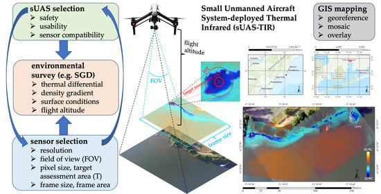
3. Proposed Methodologies

The use of sUAS-TIR to image SGD requires a thorough understanding of several key concepts, including the acquisition and integration of drone, sensor, and gimbal technologies; training flight processes; and determination of sensor lens specifications based on operational limitations, and image size and resolution requirements. We address these considerations in comprehensive detail, proposing a construct for selecting an integrated sUAS-TIR system and gaining competence deploying it, and presenting a rigorous analysis for determining an appropriate sensor lens magnification. These methodologies can be modified and employed across a range of other research and industry applications that may benefit from airborne TIR, including civil engineering (e.g., bridge delamination investigations), agriculture, (e.g., plant health and vitality), and the energy sector (e.g., solar panel inspections).

3.1. sUAS-TIR Program Development and System Selection

The use of sUAS-TIR to detect and characterize SGD requires thoughtful planning and consideration of a variety of system design factors, including the type of sUAS system, visual and TIR sensors, and sensor gimbals to deploy; the TIR sensor specifications (resolution and lens FOV/magnification); the ideal operational flight altitude; and the implementation of training and operational flight protocols for the research operations. Regulatory requirements of the governing federal, state, and local authorities—from the FAA to the sponsoring university or agency—must also be closely adhered to, though will not be discussed in detail in this paper.
Although the sUAS system, visual and TIR sensor, and sensor gimbals are often purchased as independent units, they must interface effectively as part of a whole, integrated sUAS-TIR system. The integrated nature of these components therefore requires a systems-based approach when considering their acquisition and deployment.

3.1.1. sUAS-TIR System Constraints

Selection of the combined sUAS, visual and TIR sensors, and sensor gimbals will require meeting several constraints to enable safe and effective overwater research operations. The sUAS must automatically (without manual flight control inputs) maintain a reliable, geostationary hover position and hover orientation. Automatic flight planning and execution should also be available, enabling the sUAS hover position and orientation to be recorded and replicated on subsequent flights. This requires reliable GPS positioning, auto-hover capabilities, and an onboard flight planning or flight management system. These automatic position-keeping and flight planning capabilities allow for repeatability of data/image acquisition, which is necessary for time series data or data duplicates on subsequent flights. These capabilities are also important for enabling collocated visual and TIR photos, image overlap of adjacent photos, and accurate georeferencing for image processing.
The sUAS system must simultaneously support both visual and TIR sensors, allowing for collocated visual and TIR images to be acquired and analyzed. The ability to take concurrent and collocated visual and TIR images also promotes improved situational awareness for the system operators, as well for researchers during the TIR image processing. The visual and TIR sensors must also record, or “geotag”, the sUAS position and orientation to each image, necessary for image processing and mosaicking.
The sUAS must detect and report altitude above surface waters. Altitude above surface waters is necessary to ensure TIR frame and pixel sizes can be calculated for all images (discussed in detail later, in Section 3.2.3). This altitude may be different than the GPS and/or barometric altitude above launch location reported by some sUAS systems, and may require mounting of an after-market sensor, such as a downward-looking radio altimeter.

3.1.2. sUAS-TIR System Criteria

For systems that meet the above constraints, cost–benefits can be further assessed using several sUAS-TIR system selection criteria. Though not an all-inclusive list, some of these criteria are discussed here. The sUAS-TIR system should be relatively easy to fly, particularly in a hover. For example, sUAS systems with vision positioning systems can provide measurable increases in the stability and ease of hover operations, which is essential for safe and successful image acquisition.
The sUAS-TIR system should have robust safety features, including automatic obstacle avoidance, low battery and/or loss of telemetry automatic return functions, and telemetry interference protections. These safety protections are critical in preventing flight mishaps and potentially catastrophic system loss due to collision, loss of battery life, or loss of aircraft control. Regarding telemetry interference protections, sUAS have been known to experience erratic flight behaviors when operating near significant sources of electromagnetic interference (EMI) in the sUAS telemetry transmission range (commonly 2.4 GHz or 5.8 GHz). This can bear potentially catastrophic and costly results for a sUAS-TIR system. Consequently, it is ideal to deploy a sUAS designed to protect against control/telemetry interference, such as one that employs low-latency, dual frequency telemetry, which improves control response and signal stability, and “ensures a more reliable connection in environments with interference” [27].
The sUAS-TIR system should have sufficient flight range and endurance to allow the sUAS-TIR system to takeoff, rapidly transit to the research site(s), remain on scene in a hover for enough time to gather TIR and visual photos, and return with adequate reserve flight time to ensure a sufficient safety margin. Increased flight endurance also improves the opportunity to complete multiple SGD photo operations during one flight, and therefore under relatively homogeneous environmental conditions (previously discussed).

3.1.3. sUAS-TIR Evaluation and Training

To evaluate the above sUAS-TIR system constraints and criteria, and to gain comfort and competence with sUAS-TIR system operations, sUAS-TIR systems should be test-flown following aviation’s “crawl-walk-run” training philosophy. This philosophy involves conducting flight operations in benign and controlled environments first, and incrementally increasing the environmental and flight regime challenges, until operational flights are eventually simulated in an overland training environment. Only after the team has gained significant competence in these simulated, overland training flights should overwater operational research flights, launching from the study’s research launch sites, be conducted.
Initial training flights should be conducted with the sUAS visual camera for added situational awareness, but without the TIR sensor and gimbal system attached. The TIR sensor and gimbal system can decrease flight and ground stability and control authority/maneuverability by altering the sUAS center of gravity, and interfere with stabilizing vision positioning sensors. Additionally, given the significant cost of a TIR sensor and gimbal system—often greater than that of the sUAS aircraft—flying with the TIR sensor and gimbal can unnecessarily increase the cost-based risk of a training evolution. As such, it is important to first gain competence with the sUAS system (including the visual camera/gimbal system) by conducting initial training flights without the TIR/gimbal system attached.
Initial training flights should be to a low hover, conducted outdoors in fair weather, with no precipitation and calm winds, and with fully functioning automatic hover position-keeping. These flights will allow the operators to become comfortable with the aircraft’s hover flight and position-keeping characteristics. Thereafter, training flights can be conducted to forward flight (again without the TIR/gimbal system, and in fair weather conditions). These training flights should be focused on gaining confidence and familiarity with the aircraft’s telemetry, range and endurance, in-flight maneuvering and hover transitioning characteristics, and safety features. Finally, the sUAS automatic flight planning capabilities should be practiced, allowing the end-user to gain confidence programming designated coordinates for the aircraft to automatically fly to and hover at, simulating repeatable data acquisition points for an operational flight. After the flight team has gained substantial confidence in the aforementioned flight regimes, they should be repeated, in order, with the TIR/gimbal system attached to the sUAS. These flights should be focused on learning to safely manage the sUAS aircraft, visual camera/gimbal, and TIR/gimbal systems concurrently, which may require the coordination of two or more control interfaces and system operators. Special consideration should also be given to understanding and safely managing any changes in aircraft flight characteristics and stability after adding the TIR/gimbal system.
A flow chart depicting this sUAS-TIR selection, evaluation and training process is shown in Figure 3.

3.2. TIR Specifications and Selection Criteria

There may be a number of TIR systems that are compatible with the sUAS platform. Accordingly, and in addition to evaluating the sUAS-TIR system as an integrated whole (as discussed previously), compatible TIR systems should be individually assessed to ensure they meet necessary sensor design constraints and criteria.

3.2.1. TIR Sensor Constraints

The TIR sensor must, first and foremost, be compatible with a sUAS that satisfies the aforementioned sUAS-TIR whole-system constraints and criteria (Figure 3). The TIR sensor must be bench-test compatible (i.e., capable of being powered and operated with a hand-held adaptor), allowing for education and training in low-risk, non-flight environments. The ability to operate the TIR-gimbal system from a powered, but grounded and stationary, sUAS may be a suitable substitute to this capability. The TIR sensor must be capable of providing radiometric (pixel-by-pixel) thermal data, permitting each pixel of the TIR images to serve as a discrete temperature data point and allowing for quantitative analysis, at the pixel resolution, of these data.

3.2.2. TIR Sensor Criteria

The TIR sensor should have the highest spatial resolution deemed economically feasible. Additionally, the TIR sensor lens FOV should be selected in consideration of the trade-off between image resolution and frame size, each of which are functions of both FOV and sensor distance from the emitting source (or flight elevation above water surface in the case of SGD research operations).
TIR resolution, TIR lens FOV, and TIR sensor distance from the emitting source work together to produce a given frame size and resolution, or pixel size. These factors and their relationships are discussed in the following sections of this paper.

3.2.3. TIR Resolution and FOV

Radiometric TIR sensors provide temperature data associated with each pixel in an image. This temperature data, discretized by pixel, varies across the TIR image, and provides the spatial information necessary to identify temperature differentials that may be associated with SGD. Consequently, pixel size/resolution is an important quantity to consider when using TIR to identify and quantify temperature contrasts. In general, pixel size must be significantly smaller than the size of potential SGD plumes in order to capture and quantify temperature differentials across the borders of those zones.
Determining the best sensor resolution and lens FOV for the application of TIR to SGD requires the consideration of three covarying variables: sensor distance (from the emitting source), image frame size, and pixel size/resolution. TIR sensors typically operate with a fixed lens, and thereby with a fixed optical magnification and field of view (FOV). For a given lens FOV and sensor resolution, the image frame size, f, and pixel size, p, for the TIR sensor can be calculated per Equations (8) and (9), respectively, as a function of sensor distance, R (Figure 4):
x R = t a n ( F O V 2 )
f = 2 x = 2 Rtan ( FOV 2 ) , [ m ]
p = f resolution = 2 Rtan ( FOV 2 ) resolution , [ m ]
As shown in Equations (8) and (9), decreasing the sensor distance (R) for a given sensor FOV and sensor resolution decreases both the image frame size (f) and the pixel size (p), thereby increasing the image spatial resolution. Comparing FLIR VuePro IR sensors at 336 (Table 1a) and 640 (Table 1b) resolutions, operating at the same sensor distance of 122 m (corresponding with the maximum permissible sUAS flight altitude of 400 ft), and having similar FOV angles of 45° and ~35° (corresponding with the 6.8 mm and 13 mm lens FOVs for the FLIR Vue ProR 336 and 640, respectively): although the image frame sizes are nearly identical (101 m × 80 m), the pixel sizes of the 640 resolution IR camera, approximately 0.16 m × 0.16 m, are almost ½ that of the 336 resolution camera, at approximately 0.30 m × 0.30 m. Moreover, because of a phenomenon known as the “spot effect”, wherein temperature accuracy is distorted by several optical effects as well as sensor image processing limitations, TIR technical guidelines recommends that the object or distinct thermal region being assessed (in this case the border of an SGD plume) be at least 10 pixels in diameter to achieve reliable TIR temperature information within that region [26]. This target assessment area, T, is shown in Equation (10).
T = π ( 10 p 2 ) 2 , [ m 2 ]
Equation (10) approximates the minimum target assessment area to achieve accurate TIR temperature information as the area of a circle having a diameter of 10 pixels [26]. Referring back to the aforementioned example, a 640 resolution TIR sensor operated at an altitude of 122 m (having pixel sizes of 0.16 m × 0.16 m) can therefore be expected to yield reliable temperature data for regions of approximately T = 2 m2 or greater, per Equation (10). This target assessment area increases significantly to T = 7 m2 for a 336 resolution TIR sensor at the same altitude of 122 m. These examples highlight the importance of using a higher resolution TIR sensor (e.g., 640 × 512 vs. 336 × 256), when economically feasible, to capture and quantify temperature variations across SGD plume borders, where convective mixing can yield significant temperature changes over relatively small distances [23].

3.2.4. Sensor FOV Selection Criteria

TIR sensors operate with a fixed lens, and thereby with a fixed optical magnification and field of view (FOV). Selection of the appropriate FOV for the TIR sensor requires close consideration of the sensor distance and the corresponding image frame size and spatial resolution (discussed above). As shown above, decreasing the sensor distance for a given TIR system (having a specific FOV and sensor resolution) improves spatial resolution. However, this gain comes with several costs, including: increased risk due to increased proximity to obstacles at the lower flight altitude, reduced frame size, and potentially reduced thermal accuracy due to receipt of thermal background reflections [26]. Similarly, selecting a larger lens FOV (smaller FOV angle) for a given sensor distance improves spatial resolution, but reduces the frame size and total coverage area. Smaller frame sizes necessitate a greater number of photos be taken to cover a given assessment region, which imposes survey challenges including: increased survey time requirement, difficulty surveying within a limited time window (pertinent to sUAS battery endurance and/or environmental limitations), and difficulty achieving relatively homogeneous environmental conditions across the survey region. The trade-off between frame size and spatial resolution, as determined by both the lens FOV and the sensor distance, constitutes important, competing factors that must be properly balanced through thorough consideration.
The recommended first step in selecting the best sensor FOV is to determine a minimum flight altitude (minimum sensor distance) commensurate with safe flight operations, safety being the paramount consideration for any sUAS-TIR flight operation. Specifically, the minimum safe altitude should allow sufficient clearance from ground obstacles and continuous visual contact to be maintained between the sUAS and the flight crew. Obstacles located between the launch/control site and the data acquisition location(s) can often impede visual contact with the sUAS, as required by 14 C.F.R. § 107, necessitating a higher altitude [25]. A maximum safe altitude should also be selected, with 400 ft above the surface as a default maximum safe altitude, and lower maximum safe altitudes if operating below the floor of controlled airspace [25]. As operating environments are inherently variable, a suite of minimum and maximum safe flight altitudes may be appropriate to consider, specific to different launch sites and study areas. Each minimum safe altitude to maximum safe altitude yields a sensor distance range to consider for lens FOV selection.
For each flight altitude/sensor distance minimum and maximum, a sensor FOV could be selected such that the image frame area, F, is significantly larger than the maximum estimated SGD TIR plume area, and the target assessment area, T, is significantly smaller than the minimum estimated SGD TIR plume area. In mathematical terms, and implementing the concepts from previous sections, we want to simultaneously assess Equations (11) and (12), attempting to maximize the argument (argmax) of each equation, as:
argmax { F SGD max } , [ m 2 ]
argmax { SGD min 10 T } , [ m 2 ]
where:
F = frame area = fwidth × fheight, [m2]
T = target assessment area (Equation (10)), [m2]
SGDmax = estimated upper limit of SGD TIR plume areas, [m2]
SGDmin = estimated lower limit of SGD TIR plume areas, [m2]
Note that for SGD assessments, because we require ample information to quantify temperature gradients across the SGD plume boundary region, in Equation (12) the target assessment area, T, is multiplied by an additional, subjective scaling factor of 10. The result, 10T, is then compared against SGDmin [m2], where SGDmin should be sufficiently greater than 10T. Though not shown here, when comparing these maximization functions it may also be appropriate to assign weighting factors to Equations (11) and (12) to reflect the relative importance of frame size (via Equation (11)) and pixel size (via Equation (12)) to the individual user.
Though SGD TIR plume areas vary greatly, previous studies indicate that ~5000–10,000 m2 is a reasonable upper-limit to account for most larger SGD TIR plumes, and ~50–100 m2 a reasonable lower-limit to represent smaller SGD TIR plumes [20,23,28]. Using these upper and lower limits for SGD TIR plume areas (SGDmax and SGDmin, respectively), we assess Equations (11) and (12) for 3 FOVs at altitudes from 0 m to 122 m (400 ft). Figure 5 shows F (frame area) and 10T (10× target assessment area) as a function of sensor distance (altitude) for both 336 × 256 (Figure 5a) and 640 × 512 (Figure 5b) resolution TIR sensors, where in each plot results are depicted for 3 FOVs. The blue highlighted zones on these figures depict SGDmin and SGDmax, allowing graphical comparison of F and 10T to our estimated SGDmax and SGDmin, per the arguments of Equations (11) and (12). At a given sensor distance, R, and lens FOV, if F (Figure 5, left plots) is in the blue or (more favorably) the green region it should be capable of capturing large TIR plumes in a single frame. Similarly, if 10T (Figure 5, right plots) is in the blue or (more favorably) the green region, TIR images should be of sufficiently high resolution to quantify thermal gradients at SGD TIR plume boundaries.
At the maximum permissible sUAS altitude of 122 m, favorable F and 10T values are shown for the 336 × 256 resolution sensor with 6.8 mm FOV, and for the 640 × 512 resolution sensor with both 9 mm and 13 mm FOVs. For the 336 × 256 resolution sensor (Figure 5a) with 6.8 mm FOV, at 122 m this configuration should deliver both a large enough F to capture larger plumes and a small enough 10T to resolve smaller plumes (both in their respective blue regions). By comparison, the 640 × 512 resolution sensor (Figure 5b) with 9 mm FOV provides both increased coverage (F) and slightly better resolution (10T) (shown in their green and blue regions, respectively). If increased resolution (smaller 10T) is desired, a reduction in sUAS altitude can bring 10T within the green region for each of these sensor and FOV configurations. Additionally, plumes exceeding F could be fully captured by overlapping and mosaicking adjacent images.
After assessing lens FOVs using Equations (11) and (12) for each sensor distance minimum and maximum, it is also necessary to consider the impacts of the desired FOV on overall flight operations. Recall from before that a larger lens FOV (smaller FOV angle) for a given sensor distance necessitates a greater number of photos be taken to cover a prescribed assessment region. This can prevent survey completion if sUAS battery endurance is limited or if survey timing is restricted for other reasons, such as environmental conditions or site access. Consequently, it may be appropriate to select a smaller lens FOV (larger FOV angle) to ensure imaging operations can be completed. Ultimately, frame size and spatial resolution must be assessed against all input parameters—sensor resolution, lens FOV, image distance (flight altitude), sensor distance (flight altitude), and sUAS and environmental limitations—to select the TIR sensor that most effectively allows for identification and quantification of SGD TIR plumes at the desired study region(s).

3.2.5. Environmental Considerations

In addition to the technical considerations explored in this paper, there are also numerous environmental considerations to account for in the successful implementation of sUAS-TIR for environmental surveys. For SGD assessments there must be a significant temperature differential between surface and groundwaters, which favors conducting such surveys towards the end of the summer (winter), when surface waters are significantly warmer (colder) than groundwaters. Additionally, lighter on-scene wind conditions promote weaker shear- and thermally induced mixing, better allowing the plume’s temperature differential to be detected by TIR [21]. During summer surveys, shading of the nearshore environment by clouds and/or coastal trees and foliage, can limit or mask the colder thermal signatures of SGD TIR plumes, particularly in the morning before the surface waters have experienced sufficient diurnal warming. Additionally, background thermal reflections and solar reflections off the water surface can impose substantial cold and hot (respectively) thermal deviations for the TIR sensor, precluding the sensor from detecting the thermal signature of the water; steeper viewing angles can help mitigate these reflection effects [26].

3.3. Quantifying SGD TIR Plume Areas

One method of calculating SGD TIR plume areas using TIR images is by quantifying the spatial temperature gradient for SGD TIR plumes along select transects orthogonal to isotherms (in the direction of greatest temperature change). The border of the SGD TIR plume can be delineated at the temperature inflection points, where the magnitude of the temperature gradient is at a maximum, given as:
| T | max
2 T r 2 = 0 , [ K m 2 ]
where T is the TIR-derived water temperature, and r is the distance along select transect(s). As the inflection point is both quantifiable and exists centrally within a spatially constrained zone between two distinct thermal regions (SGD plume and background waters), it provides an ideal demarcation of the two regions. A graphical depiction of this method is shown in Figure 6. This method could be applied to both point and diffuse SGD plume sources. For broad diffuse sources, it may be preferred to average the temperature inflection points from more than one transect.
SGD TIR plume areas from TIR can then be calculated as the number of image pixels at or below the inflection temperature (Equation (13)) multiplied by the pixel area. This general method has been successfully used in previous airborne-TIR work to determine the borders of cooler groundwater discharge plumes against warmer surface waters and to calculate the area of the identified plumes.
A flow chart reflecting the TIR sensor selection process described above is shown in Figure 7. This flow chart is a first-draft methodology for selecting a suitable sensor. As knowledge increases about the study region and operational environment, and the remote sensing challenges and limitations imposed by these environments are better understood, this flow chart can be appropriately modified.

3.4. SGD TIR Plume Examples Using sUAS-TIR

As one example of sUAS-TIR technology applied to SGD identification and characterization, Figure 8 depicts two adjacent and overlapping TIR images showing multiple TIR plumes of SGD sources along the shoreline of a coastal estuary in southern Rhode Island, USA. The survey was conducted from a DJI Inspire 1 drone flown at 122 m (400 ft) above the surface, using a FLIR Vue Pro R (radiometric) 336 camera with 6.8 mm lens FOV for the TIR images, and a Zenmuse XT for the visual images. At the flight altitude (image distance) of 122 m, each TIR image has a coverage (frame size) of 101.0 m × 76.9 m, or 7765.3 m2; a pixel size of 0.3 m × 0.3 m; and a target assessment area of 7.1 m2 (Table 1a). The blue (colder) hues indicate SGD with ample terrestrially derived fresh groundwater component to ensure buoyancy-driven advection to the surface and a significant thermal differential with the background surface waters. The rightmost plume appears to originate from a point source, whereas the other plumes appear to derive from diffuse sources. The different temperatures of the plumes—noting that the coldest plume is 12.9 °C in the left TIR image and 14.9 °C in the right image—likely indicate distinct source characteristics, such as depth of originating terrestrial groundwaters, compositional fractions of fresh groundwater, and SGD/surface water mixing dynamics. The collocated visual photos enable improved analysis of the TIR images for SGD, including assessment of potential confounding effects such as shading from coastal foliage and low emissivity materials. For example, the dark blue rectangle located at 41°22′51″ N, 71°38′49.5″ W (Figure 8) can be identified as a metal dock, vice SGD. Due to having a lower emissivity, e, than water, and a high reflectivity that can transmit the (cold) atmospheric background signal [26], the metal dock will emit significantly less power in the infrared spectrum for a given temperature (Equation (6)) and therefore will falsely present as a cold artifact.

4. Applications and Opportunities

The use of TIR to identify and characterize SGD plumes in previous studies has uncovered a consistent, significant correlation between SGD flux and SGD TIR plume area. This strong relationship, coupled with the capability of sUAS-TIR to deliver SGD data at unusually high spatial resolutions and sub-daily temporal resolutions, presents several novel opportunities for future developments in this field.

4.1. Airborne TIR SGD Studies

Though numerous studies have used airborne TIR to assess SGD, based on current literature reviews, only two studies report the use of sUAS-TIR technologies for SGD [20,29], with a few additional studies characterizing groundwater discharges into fresh water bodies using sUAS-TIR [30,31]. TIR can be used to identify and quantify SGD surface plume areas; however, it is unable to directly resolve SGD plume fluxes. Accordingly, several studies have coupled the use of TIR to determine SGD plume area with well-established in situ methods of calculating SGD fluxes [19,20,23,28,32,33]. Though these studies assessed SGD in different regions and using different empirical methods, all reported a strong regression between SGD flux (via in situ data) and SGD TIR plume area (via airborne TIR) for each assessed region (Table 2).
These regressions appear to exist for both total SGD flux and for freshwater SGD flux [28], and the regression relationships are predominantly linear for total SGD [19,20,23,32,33], with one study of freshwater SGD finding a logarithmic relationship [28]. Additionally, the relationships appear to be regionally specific, with different regression slopes for different study areas [19,20,23,28,32,33], indicating specific hydrogeological and geomorphological controls to the SGD flux vs. plume area regression [19,23,33].

4.2. sUAS-TIR SGD Research Opportunities

The proven efficacy of sUAS-TIR to detect and quantify SGD bares exciting prospects for additional contributions to this field. We discuss a few of these novel research opportunities below.

4.2.1. Coastal Estuaries

One particular opportunity for novel application of sUAS-TIR is in coastal lagoons and estuaries. Only one study has used sUAS-TIR in combination with in situ measurements to quantify flux [20], and though few studies have used TIR coupled with in situ measurements to quantify SGD in coastal estuaries [19,28,34] none have yet done so using sUAS-TIR. Moreover, as noted in previous assessments of SGD, the highly variable and heterogeneous nature of SGD makes it difficult to quantify total volumetric discharge and necessitates thorough identification of SGD discharge locations to guide data acquisition [35,36]. sUAS-TIR can directly support such studies in sensitive coastal ecosystems through the identification, mapping, and characterization of SGD point and diffuse discharge zones, as important potential sources of terrestrially derived pollutants, and enabling targeted radionuclide tracer data acquisition to facilitate more accurate in situ SGD flux measurements. The lower salinity gradient between fresh SGD and the brackish waters of lagoons and estuaries, in comparison with that of fresh SGD in ocean waters, may produce subdued exhibition of thermal plumes due to reduced buoyancy. Non-dimensional physical flow assessments, including buoyancy vs. conduction (Rayleigh number) and buoyancy vs. mixing (Richardson number) should be conducted to approximate the characteristics—including salinity/density differential, temperature differential, and depth—wherein the SGD effluent would likely be detectable on the surface of the estuary or lagoon [21].

4.2.2. Total and Fresh SGD vs. TIR Plume Area Regressions

Additional TIR assessments of SGD coupled with in situ measurements, and comparison to previous studies, are necessary to better understand the flux vs. plume area regression and its controls at study sites of varying hydrogeology. As the regression equations will be different for total SGD flux (recirculated saline or brackish porewaters in combination with terrestrially derived fresh groundwaters) vice the fresh fraction of SGD flux, in situ assessments of both are necessary. The current lack of studies providing regressions for both total SGD and fresh SGD thereby presents an important research opportunity. As the SGD flux vs. SGD TIR plume area regressions and their controls are better understood, sUAS-TIR detection may provide a parsimonious means for scientists and resource managers to assess SGD fluxes in regions where in situ measurements are environmentally or logistically prohibitive—an important capability given the significance of SGD as a chemical and nutrient transport mechanism [4,8].

4.2.3. Hydrogeologic Controls

The dependence of regression slopes on locality indicates the possibility of one or more hydrogeologic controlling factors. Hydrogeologic factors have yet to be analyzed in combination with flux and plume area. Factors such as conductivity, storativity, porosity, hydraulic gradient, and onshore topography [23,33,34] should be assessed in company with regression slopes to better constrain the SGD flux vs. plume area relationship. To evaluate hydrogeologic factors and their spatial variability, temporal variabilities have to be controlled over a suite of study sites. One means of accomplishing this is by assessing SGD TIR plume areas at approximately equal tidal stages and seasons for all study regions and comparing these SGD TIR plume areas to concurrently measured or time-averaged fluxes. If definitive hydrogeologic factors can be identified and quantified as controls to the SGD flux vs. plume area regression slope, this may enable the application of regionally specific regression curves to SGD TIR plume area to approximate regional SGD fluxes, without the need for time consuming in situ measurements.

4.2.4. Temporal Dynamics

SGD flux and SGD TIR plume areas are sensitive to temporal dynamics that operate on seconds to annual timescales. For example, plume area may vary with temperature differential between SGD and surface waters [23], while SGD flux is dependent on other temporal factors including wave action, tidal pumping, salinity/density gradient, and seasonal recharge [2,12,37]. Quantifying flux vs. plume areas at select “end-member” seasonal and/or tidal cycles (e.g., peak summer, peak winter; high, low, and slack tides) for one or more specific study regions may be an appropriate first-order analysis of temporal controls on the flux vs. plume area regression, and to our knowledge has not yet been undertaken. As none of these studies (Table 2) reported concurrent flux and plume areas over a range of tidal and seasonal conditions, the temporal co-dependence of SGD flux and plume area is not well-understood and warrants evaluation. Several studies have successfully quantified detectable SGD TIR plumes across all tidal ranges [20,22], indicating this to be a reasonable pursuit.

4.2.5. Solving for Fresh SGD Flux Using the Dupuit-Ghyben-Herzberg Model

If strong linear regressions exist for fresh SGD flux vs. SGD TIR plume area, either temporally (i.e., at different tidal stages for a single plume), or spatially (i.e., across multiple SGD plumes within a hydrogeologically constrained region), then the following general equation will apply:
Q n = mA n + b , [ m 3 / day ]
where Qn is freshwater SGD volumetric discharge for plume n, b is the regression y-intercept (representing the lower SGD flux threshold below which a SGD TIR plume does not present), An is SGD TIR plume area, m is the regression slope, and n is the temporally or spatially specific data point (discretized by time at a single plume for a temporal regression; discretized by plume at a specific time for a spatial regression within a study region).
If this linear regression is found to hold consistently for fresh SGD flux vs. SGD TIR plume area, then the freshwater SGD flux, Qn, can be computationally solved as a system of nonlinear equations, without requiring in situ empirical SGD flux measurements, by applying Glover’s (1959) modified solutions to the Dupuit-Ghyben-Herzberg model, Equation (15) [38,39].
h n = 2 x n Q n G K = 2 x n ( Q n L n ) G K ,     [ m ]
where K is hydraulic conductivity [m/day], Q′n is freshwater SGD volumetric discharge (Qn) per length of coastline (Ln) in [m2/day], hn is the groundwater table height above sea level measured a linear distance xn from the shoreline, and G (Equation (16)) accounts for the density difference between the fresh porewaters, ρ f , and the saline background waters, ρ s [39]:
G = ρ f ρ s ρ f
By measuring the following variables at an SGD TIR plume site at three or more n values:
  • An, SGD TIR plume area
  • Ln, SGD TIR plume coastline length
  • G, fresh and saltwater densities (Equation (16)),
  • hn, water table height (h), and
  • xn, distance of water table or fresh-saltwater interface measurement from shoreline.
The freshwater SGD flux, Qn, can then be solved by applying three An values to Equations (14) and (15) to create a system of equations that can be regressed for m, b, K, and Qn, and therefore used to solve for the freshwater SGD fluxes of each plume.

4.2.6. Climate Change

The effects of climate change and climate-sensitive environmental factors on SGD—including groundwater levels, mean tidal stage and tidal dynamics, and coastal groundwater salinization—are not well understood. The continued application of sUAS-TIR to SGD assessments will improve our understanding of various environmental controls on SGD fluxes and their spatial and temporal dynamics, providing valuable insights into the potential impacts of climate change on SGD and on SGD-advected nutrient fluxes [40]. In doing so, sUAS-TIR technology stands to advance our understanding of SGD with important implications.

5. Conclusions

The ability for TIR to detect SGD surface plumes presents important opportunities for SGD research. When coupled with airborne deployment methods, TIR can provide continuous coverage of large areas at high spatial resolution, offering a means to qualitatively identify point and nonpoint/diffuse SGD zones for in situ data collection and address spatial scaling challenges of empirical SGD analyses. Given the developing technology and reduced operating costs of sUAS, as well as the increased operational flexibility associated with this technology, sUAS-TIR stands to bolster TIR capabilities for SGD surface data acquisition—increasing spatial resolution and temporal-targeting. Developing sUAS-TIR technology for SGD assessments requires thorough consideration of a number of factors, including the sUAS, sensor, and gimbal systems to deploy, training procedures and protocols, operational flight regimes, and sensor lens selection that achieves an appropriate balance between image size and spatial resolution. Rigorous, well-informed attention to these factors can ensure a sUAS-TIR system is deployed that allows for successful identification and quantification of SGD TIR plumes, with relevance to a variety of other academic and industrial applications. Initial studies of SGD flux and SGD TIR plume area have uncovered a consistent, strong regression between flux and plume area, indicating the potential to use sUAS-TIR directly for SGD flux analysis and quantification. However, spatial and temporal controls on this relationship have not yet been assessed. Spatially, the regional variability of flux vs. plume area regressions point to potential hydrogeologic controls on this regression that have not been isolated and quantified; temporally, though previous studies compared non-concurrent or time-averaged flux vs. plume area, or assumed a regression that was constant in time, the temporal co-dependence of SGD flux and plume area is currently not known and warrants evaluation. Coupling sUAS-TIR with empirical studies of SGD flux will enable quantification of spatial and temporal variability and identification of controls, as well as the pursuit of other novel methods and findings, including quantification of seasonal and tidal SGD flux dynamics. As our understanding of the SGD flux vs. SGD TIR plume area relationship and its spatial and temporal controls grows, sUAS-TIR may become an independent means to assess SGD fluxes in regions and/or at scales for which in situ measurements are prohibitive.

Author Contributions

Conceptualization, S.M.P. and K.S.R.Y.; methodology, K.S.R.Y.; writing—original draft preparation and analysis, K.S.R.Y.; writing—review and editing, S.M.P. and K.S.R.Y.; supervision, S.M.P.; project administration, S.M.P.; funding acquisition, S.M.P. All authors have read and agreed to the published version of the manuscript.

Funding

“This research was funded by Rhode Island Housing and Urban Development, grant number 13/URI/DR-01”; USDA NIFA S-1089 Multistate Hatch Grant; and the United States Coast Guard Academy.

Acknowledgments

The authors would like to thank Janelle Kmetz, Jeeban Panthi, and residents of Charlestown, RI and South Kingstown, RI for the support we received during this research project.

Conflicts of Interest

The authors have no conflict of interest to declare.

References

  1. Burnett, W.C.; Bokuniewicz, H.; Huettel, M.; Moore, W.S.; Taniguchi, M. Groundwater and pore water inputs to the coastal zone. Biogeochemistry 2003, 66, 3–33. [Google Scholar] [CrossRef]
  2. Burnett, W.; Aggarwal, P.; Aureli, A.; Bokuniewicz, H.; Cable, J.; Charette, M.; Kontar, E.; Krupa, S.; Kulkarni, K.; Loveless, A.; et al. Quantifying submarine groundwater discharge in the coastal zone via multiple methods. Sci. Total. Environ. 2006, 367, 498–543. [Google Scholar] [CrossRef]
  3. Tovar-Sánchez, A.; Basterretxea, G.; Rodellas, V.; Sánchez-Quiles, D.; García-Orellana, J.; Masqué, P.; Jordi, A.; López, J.M.; Garcia-Solsona, E. Contribution of Groundwater Discharge to the Coastal Dissolved Nutrients and Trace Metal Concentrations in Majorca Island: Karstic vs Detrital Systems. Environ. Sci. Technol. 2014, 48, 11819–11827. [Google Scholar] [CrossRef] [Green Version]
  4. Oberdorfer, J.A. Hydrogeologic Modeling of Submarine Groundwater Discharge: Comparison to Other Quantitative Methods. Biogeochemistry 2003, 66, 159–169. [Google Scholar] [CrossRef]
  5. Church, T.M. An underground route for the water cycle. Nat. Cell Biol. 1996, 380, 579–580. [Google Scholar] [CrossRef]
  6. Kwon, E.Y.; Kim, G.; Primeau, F.; Moore, W.S.; Cho, H.; Devries, T.; Sarmiento, J.L.; Charette, M.A.; Cho, Y. Global estimate of submarine groundwater discharge based on an observationally constrained radium isotope model. Geophys. Res. Lett. 2014, 41, 8438–8444. [Google Scholar] [CrossRef]
  7. Taniguchi, M.; Burnett, W.C.; Cable, J.E.; Turner, J.V. Investigation of submarine groundwater discharge. Hydrol. Process. 2002, 16, 2115–2129. [Google Scholar] [CrossRef]
  8. Sawyer, A.H.; David, C.H.; Famiglietti, J.S. Continental patterns of submarine groundwater discharge reveal coastal vulnerabilities. Science 2016, 353, 705–707. [Google Scholar] [CrossRef] [Green Version]
  9. Knee, K.L.; Street, J.H.; Grossman, E.E.; Boehm, A.B.; Paytan, A. Nutrient inputs to the coastal ocean from submarine groundwater discharge in a groundwater-dominated system: Relation to land use (Kona coast, Hawaii, U.S.A.). Limnol. Oceanogr. 2010, 55, 1105–1122. [Google Scholar] [CrossRef] [Green Version]
  10. Dulaiova, H.; Camilli, R.; Henderson, P.B.; Charette, M.A. Coupled radon, methane and nitrate sensors for large-scale assessment of groundwater discharge and non-point source pollution to coastal waters. J. Environ. Radioact. 2010, 101, 553–563. [Google Scholar] [CrossRef]
  11. Moore, W.S. The Effect of Submarine Groundwater Discharge on the Ocean. Annu. Rev. Mar. Sci. 2010, 2, 59–88. [Google Scholar] [CrossRef] [PubMed] [Green Version]
  12. Michael, H.A.; Mulligan, A.E.; Harvey, C.F. Seasonal oscillations in water exchange between aquifers and the coastal ocean. Nat. Cell Biol. 2005, 436, 1145–1148. [Google Scholar] [CrossRef] [PubMed]
  13. Michael, H.A.; Charette, M.A.; Harvey, C.F. Patterns and variability of groundwater flow and radium activity at the coast: A case study from Waquoit Bay, Massachusetts. Mar. Chem. 2011, 127, 100–114. [Google Scholar] [CrossRef]
  14. Prieto, C.; Destouni, G. Is submarine groundwater discharge predictable? Geophys. Res. Lett. 2011, 38. [Google Scholar] [CrossRef]
  15. Smith, L.; Zawadzki, W. A hydrogeologic model of submarine groundwater discharge: Florida intercomparison experiment. Biogeochemistry 2003, 66, 95–110. [Google Scholar] [CrossRef]
  16. Robinson, C.; Li, L.; Prommer, H. Tide-induced recirculation across the aquifer-ocean interface. Water Resour. Res. 2007, 43. [Google Scholar] [CrossRef] [Green Version]
  17. Anderson, M.P. Heat as a Ground Water Tracer. Ground Water 2005, 43, 951–968. [Google Scholar] [CrossRef] [PubMed]
  18. Chuvieco, E. Fundamentals of Satellite Remote Sensing: An Environmental Approach, 2nd ed.; Taylor & Francis Group: Boca Raton, FL, USA, 2016. [Google Scholar]
  19. Bejannin, S.; Van Beek, P.; Stieglitz, T.; Souhaut, M.; Tamborski, J. Combining airborne thermal infrared images and radium isotopes to study submarine groundwater discharge along the French Mediterranean coastline. J. Hydrol. Reg. Stud. 2017, 13, 72–90. [Google Scholar] [CrossRef]
  20. Lee, E.; Yoon, H.; Hyun, S.P.; Burnett, W.C.; Koh, D.; Ha, K.; Kim, D.; Kim, Y.; Kang, K. Unmanned aerial vehicles (UAVs)-based thermal infrared (TIR) mapping, a novel approach to assess groundwater discharge into the coastal zone. Limnol. Oceanogr. Methods 2016, 14, 725–735. [Google Scholar] [CrossRef]
  21. Lewandowski, J.; Meinikmann, K.; Ruhtz, T.; Pöschke, F.; Kirillin, G. Localization of lacustrine groundwater discharge (LGD) by airborne measurement of thermal infrared radiation. Remote Sens. Environ. 2013, 138, 119–125. [Google Scholar] [CrossRef]
  22. McCaul, M.; Barland, J.; Cleary, J.; Cahalane, C.; McCarthy, T.; Diamond, D. Combining Remote Temperature Sensing with in-Situ Sensing to Track Marine/Freshwater Mixing Dynamics. Sensors 2016, 16, 1402. [Google Scholar] [CrossRef] [PubMed] [Green Version]
  23. Tamborski, J.J.; Rogers, A.D.; Bokuniewicz, H.J.; Cochran, J.K.; Young, C.R. Identification and quantification of diffuse fresh submarine groundwater discharge via airborne thermal infrared remote sensing. Remote Sens. Environ. 2015, 171, 202–217. [Google Scholar] [CrossRef] [Green Version]
  24. General Operating and Flight Rules, 14 C.F.R. § 91. 2021. Available online: https://www.ecfr.gov/cgi-bin/text-idx?node=14:2.0.1.3.10 (accessed on 28 January 2021).
  25. Small Unmanned Aircraft Systems, 14 C.F.R. § 107. 2021. Available online: https://www.ecfr.gov/cgi-bin/text-idx?node=pt14.2.107&rgn=div5 (accessed on 28 January 2021).
  26. FLIR. Technical Note: Radiometric Temperature Measurements. 2016. Available online: www.flir.com/suas (accessed on 8 September 2020).
  27. DJI. Matrice 200 Series V2, M210 V2/M210 RTK V2, User Manual v1.4. 2019. Available online: https://www.dji.com/matrice-200-series-v2/info#downloads (accessed on 4 January 2021).
  28. Danielescu, S.; MacQuarrie, K.T.B.; Faux, R.N. The integration of thermal infrared imaging, discharge measurements and numerical simulation to quantify the relative contributions of freshwater inflows to small estuaries in Atlantic Canada. Hydrol. Process. 2009, 23, 2847–2859. [Google Scholar] [CrossRef]
  29. Mallast, U.; Siebert, C. Combining continuous spatial and temporal scales for SGD investigations using UAV-based thermal infrared measurements. Hydrol. Earth Syst. Sci. 2019, 23, 1375–1392. [Google Scholar] [CrossRef] [Green Version]
  30. Dugdale, S.J.; Kelleher, C.A.; Malcolm, I.A.; Caldwell, S.; Hannah, D.M. Assessing the potential of drone-based thermal infrared imagery for quantifying river temperature heterogeneity. Hydrol. Process. 2019, 33, 1152–1163. [Google Scholar] [CrossRef]
  31. Ore, J.; Burgin, A.; Schoepfer, V.; Detweiler, C. Towards monitoring saline wetlands with micro UAVs. In Proceedings of the Robot Science and Systems Workshop on Robotic Monitoring, Berkeley, CA, USA, 12–16 July 2014. [Google Scholar]
  32. Kelly, J.L. Identification and quantification of submarine groundwater discharge in the Hawaiian Islands. Ph.D. Thesis, University of Hawaii, Honolulu, UI, USA, 2012. [Google Scholar]
  33. Kelly, J.L.; Glenn, C.R.; Lucey, P.G. High-resolution aerial infrared mapping of groundwater discharge to the coastal ocean. Limnol. Oceanogr. Methods 2013, 11, 262–277. [Google Scholar] [CrossRef]
  34. Mulligan, A.E.; Charette, M.A. Intercomparison of submarine groundwater discharge estimates from a sandy unconfined aquifer. J. Hydrol. 2006, 327, 411–425. [Google Scholar] [CrossRef]
  35. Scott, M.K.; Moran, S.B. Ground water input to coastal salt ponds of southern Rhode Island estimated using 226Ra as a tracer. J. Environ. Radioact. 2001, 54, 163–174. [Google Scholar] [CrossRef]
  36. Stachelhaus, S.L.; Moran, S.B.; Kelly, R.P. An evaluation of the efficacy of radium isotopes as tracers of submarine groundwater discharge to southern Rhode Island’s coastal ponds. Mar. Chem. 2012, 130–131, 49–61. [Google Scholar] [CrossRef]
  37. Li, H.; Jiao, J. Quantifying tidal contribution to submarine groundwater discharges: A review. Chin. Sci. Bull. 2013, 58, 3053–3059. [Google Scholar] [CrossRef] [Green Version]
  38. Glover, R.E. The pattern of fresh-water flow in a coastal aquifer. J. Geophys. Res. Space Phys. 1959, 64, 457–459. [Google Scholar] [CrossRef]
  39. Fetter, C.W. Applied Hydrogeology, 4th ed.; Prentice-Hall, Inc.: Upper Saddle River, NJ, USA, 2001. [Google Scholar]
  40. Johnson, A.G.; Glenn, C.R.; Burnett, W.C.; Peterson, R.N.; Lucey, P.G. Aerial infrared imaging reveals large nutrient-rich groundwater inputs to the ocean. Geophys. Res. Lett. 2008, 35. [Google Scholar] [CrossRef] [Green Version]
Figure 1. SGD to a coastal ecosystem, depicting the sub-components and processes of SGD (fresh and saline), their source reservoirs, and their driving forces [11].
Remotesensing 13 01331 g001
Adapted and modified from Moore, 2010 [11].
Figure 2. Planck’s blackbody radiation curves, depicting radiation intensity vs. wavelength for emitting surfaces at 200 K to 400 K, representing a broad range of Earth surface temperatures (Earth’s average surface temperature being approximately 288 K). Within the depicted temperature range, variations in surface temperatures yield relatively small shifts in the wavelength of peak radiation intensity (dashed line), but result in large changes to the total radiation intensity (area under each curve) within the TIR spectrum.
Remotesensing 13 01331 g002
Figure 3. sUAS-TIR flow chart, denoting constraints and criteria for sUAS-TIR system selection, and providing recommended evaluation and training methodologies for the safe inception and use of sUAS-TIR.
Remotesensing 13 01331 g003
Figure 4. Geometries for use in Equations (8) and (9) to calculate image frame size, f, and pixel size, p, as a function of FOV, sensor resolution, and sensor distance, R. These geometries are also applied in Equations (4)–(6) to calculate radiated power received by a TIR sensor from an emitting source.
Remotesensing 13 01331 g004
Figure 5. Frame area, F (left plots), and 10× target assessment area, 10T (right plots) vs. sensor distance, R, plotted for three lens FOVs. These relationships are shown for a 336 × 256 resolution TIR sensor (a) and a 640 × 512 resolution TIR sensor (b). In the left plots (F vs. R) the blue regions represent an estimated upper limit of SGD TIR plume areas. In the right plots (10T vs. R) the blue regions represent an estimated lower limit of smaller SGD TIR plume areas. At a given sensor distance, R, and lens FOV, if F, is in the green region it should be capable of capturing large TIR plumes in a single frame. Similarly, if 10T is in the green region (right plot), TIR images should be of sufficiently high resolution to identify SGD TIR plume boundaries.
Remotesensing 13 01331 g005
Figure 6. TIR-derived surface water temperatures (vertical axis) plotted vs. distance from shoreline along designated transects (horizontal axis) [23]. Solid dots depict the inflection points of temperature, where the 2nd spatial derivative of T(r) equals 0. Plume area can be calculated as the number of image pixels at or below the inflection temperature multiplied by the pixel area.
Remotesensing 13 01331 g006
Adapted and modified from Tamborski et al., 2015 [23].
Figure 7. TIR sensor selection flow chart, denoting constraints, criteria, and evaluation methodology for TIR sensor selection and use in an integrated sUAS-TIR system.
Remotesensing 13 01331 g007
Figure 8. sUAS-TIR images overlaid onto collocated visual photos, depicting examples of SGD TIR plumes that are both localized/point sourced (rightmost plume), and diffuse. The TIR survey location was the northern shore of Fort Neck Cove, Ninigret Pond, Rhode Island (RI), USA. The survey was conducted via a DJI Inspire 1 drone flown at 122 m (400 ft) above the shoreline of the brackish coastal estuary on 6 August 2020 at 1730 (EDT/local time), approximately 1.5 hours prior to estuary low tide. Blue hues (colder) indicate SGD having ample terrestrially derived fresh groundwater component. The radiometric temperatures of the coldest SGD plume in each TIR image are shown. TIR images were taken with a FLIR Vue Pro R (radiometric) 336 × 256 resolution sensor with 6.8 mm lens FOV. Visual images were taken with a DJI Zenmuse X3 4096 × 2160 resolution camera with 3.6 mm lens FOV. TIR image processing was conducted using FLIR Tools software, with additional processing and mapping of visual and TIR images in ArcGIS Pro.
Remotesensing 13 01331 g008
Table 1. Frame size, f, frame area, F, pixel size, p, and target assessment area, T, for FLIR Vue Pro 336 (a) and 640 (b) TIR cameras, as a function of camera FOV angle [degrees] and sensor distance, R [m]. TIR cameras have a fixed FOV angle. Consequently, a smaller sensor distance yields less coverage area (smaller frame size and frame area per image) but a higher spatial resolution (smaller pixel sizes and target assessment area).
(a) 336 × 256 resolution:
FRAME SIZE, f [m], VueProR 336
FRAME AREA, F [m2]
sensor distance, R [m]
lens FOVFOV angle [°]variable, dimensions153046617691107122
6.8 mm45fwidth [m]12.625.337.950.563.175.888.4101.0
35fheight [m]9.619.228.838.448.157.767.376.9
6.8 mm45 × 35Farea [m2]121.3485.31092.01941.33033.34368.05945.37765.3
9 mm35fwidth [m]9.619.228.838.448.157.767.376.9
27fheight [m]7.314.622.029.336.643.951.258.5
9 mm35 × 27Farea [m2]70.3281.3632.91125.21758.12531.73445.94500.8
13 mm25fwidth [m]6.813.520.327.033.840.547.354.1
19fheight [m]5.110.215.320.425.530.635.740.8
13 mm25 × 19Farea [m2]34.5137.9310.2551.5861.71240.81688.82205.8
PIXEL SIZE, p [m], VueProR 336
TARGET ASSESSMENT AREA, T [m2]
sensor distance, R [m]
lens FOVFOV angle [°]variable, dimensions153046617691107122
6.8 mm45pwidth [m]0.0380.0750.1130.1500.1880.2250.2630.301
35pheight [m]0.0380.0750.1130.1500.1880.2250.2630.300
6.8 mm45 × 35Tarea [m2]0.1110.4440.9981.7742.7723.9925.4347.097
9 mm35pwidth [m]0.0290.0570.0860.1140.1430.1720.2000.229
27pheight [m]0.0290.0570.0860.1140.1430.1720.2000.229
9 mm35 × 27Tarea [m2]0.0640.2570.5781.0281.6062.3133.1484.112
13 mm25pwidth [m]0.0200.0400.0600.0800.1010.1210.1410.161
19pheight [m]0.0200.0400.0600.0800.1000.1200.1390.159
13 mm25 × 19Tarea [m2]0.0320.1270.2860.5080.7941.1441.5562.033
(b) 640 × 512 resolution:
FRAME SIZE, f [m], VueProR 640
FRAME AREA, F [m2]
sensor distance, R [m]
lens FOVFOV angle [°]variable, dimensions153046617691107122
9 mm69fwidth [m]20.941.962.883.8104.7125.7146.6167.6
56fheight [m]16.232.448.664.881.097.2113.4129.7
9 mm69 × 56Farea [m2]339.51358.03055.55432.08487.512222.016635.521727.9
13 mm45fwidth [m]12.625.337.950.563.175.888.4101.0
37fheight [m]10.220.430.640.851.061.271.481.6
13 mm45 × 37Farea [m2]128.8515.01158.82060.13218.94635.36309.18240.5
19 mm32fwidth [m]8.717.526.235.043.752.461.269.9
26fheight [m]7.014.121.128.135.242.249.356.3
19 mm32 × 26Farea [m2]61.5246.0553.5984.01537.62214.13013.63936.1
PIXEL SIZE, p [m], VueProR 640
TARGET ASSESSMENT AREA, T [m2]
sensor distance, R [m]
lens FOVFOV angle [°]variable, dimensions153046617691107122
9 mm69pwidth [m]0.0330.0650.0980.1310.1640.1960.2290.262
56pheight [m]0.0320.0630.0950.1270.1580.1900.2220.253
9 mm69 × 56Tarea [m2]0.0840.3370.7571.3462.1043.0294.1235.385
13 mm45pwidth [m]0.0200.0390.0590.0790.0990.1180.1380.158
37pheight [m]0.0200.0400.0600.0800.1000.1200.1390.159
13 mm45 × 37Tarea [m2]0.0310.1220.2750.4890.7641.1001.4981.956
19 mm32pwidth [m]0.0140.0270.0410.0550.0680.0820.0960.109
26pheight [m]0.0140.0270.0410.0550.0690.0820.0960.110
19 mm32 × 26Tarea [m2]0.0150.0590.1320.2340.3660.5270.7180.937
Table 2. Studies of SGD employing TIR to assess SGD TIR plume area in combination with in situ methods of determining SGD flux. In all studies, strong regressions of SGD flux vs. SGD TIR plume area are observed across multiple plumes occurring in common regions, demonstrating SGD TIR plume area as a reliable indicator of SGD flux [19,20,23,28,32,33]. Different regression slopes between study regions indicate that the relationship between SGD flux and plume area is subject to regionally specific hydrogeologic controls.
StudyLocation(s)SGD Flux Method
(Rn = Radon Mass Balance;
Ra = Radium Mass Balance)
SGD Flux Timing
(LT = Low Tide
HT = High Tide
TA = Time-Averaged)
TIR MethodTIR Timing
(LT = Low Tide
HT = High Tide
MT = Mid-Tide)
Regression
(SGD Flux vs. Plume Area)
R2
Danielescu et al., 2009Trout River Estuary,
McIntyre Creek Estuary
(Atlantic, Canada)
current meter
(for springs);
MODFLOW/numerical (for diffuse SGD)
July 2007;
TA
manned aircraftSeptember 2005;
LT
logarithmic 0.89
Kelly et al., 2013Pearl Harbor
(HI, U.S.)
RnJanuary–March 2010;
TA
manned aircraftJuly 2009;
LT
linear0.98
Tamborski et al., 2015Port Jefferson Harbor, Smithtown Bay,
E. Suffolk County
(Long Island Sound, NY, U.S.)
Rn;
seepage meters
August 2012,
June 2013,
September 2014; TA
manned aircraftJuly 2014,
August 2013,
September 2014;
LT
linear0.94
0.93
0.81
Lee et al., 2016Gongcheonpo Beach, Jeju Island (Korea)current meterJuly 2014, August 2015; LTsUASAugust 2015; LT, HT, MTlinear0.99
Bejannin et al., 2017French Mediterranean
(France)
RaMay 2009–April 2016
(varies)
manned aircraftSeptember 2012linear0.99
Average R2:0.96
Publisher’s Note: MDPI stays neutral with regard to jurisdictional claims in published maps and institutional affiliations.

