Spatiotemporal Downscaling of GRACE Total Water Storage Using Land Surface Model Outputs

Abstract

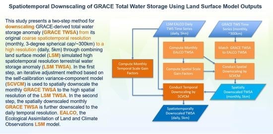
High spatiotemporal resolution of terrestrial total water storage plays a key role in assessing trends and availability of water resources. This study presents a two-step method for downscaling GRACE-derived total water storage anomaly (GRACE TWSA) from its original coarse spatiotemporal resolution (monthly, 3-degree spherical cap/~300 km) to a high resolution (daily, 5 km) through combining land surface model (LSM) simulated high spatiotemporal resolution terrestrial water storage anomaly (LSM TWSA). In the first step, an iterative adjustment method based on the self-calibration variance-component model (SCVCM) is used to spatially downscale the monthly GRACE TWSA to the high spatial resolution of the LSM TWSA. In the second step, the spatially downscaled monthly GRACE TWSA is further downscaled to the daily temporal resolution. By applying the method to downscale the coarse resolution GRACE TWSA from the Jet Propulsion Laboratory (JPL) mascon solution with the daily high spatial resolution (5 km) LSM TWSA from the Ecological Assimilation of Land and Climate Observations (EALCO) model, we evaluated the benefit and effectiveness of the proposed method. The results show that the proposed method is capable to downscale GRACE TWSA spatiotemporally with reduced uncertainty. The downscaled GRACE TWSA are also evaluated through in-situ groundwater monitoring well observations and the results show a certain level agreement between the estimated and observed trends.

1. Introduction

Accurate knowledge on total or terrestrial water storage (TWS) and its spatiotemporal variability play a crucial role in the assessment of climate variation and water resource availability [1]. The accuracy of TWS simulated by land surface models (LSMs) at high spatial and temporal resolution is commonly limited by uncertainties in meteorological forcing, model parameter calibration, and land surface process representation [2,3,4,5]. To reduce the model uncertainties, researchers have been developing new LSMs that may account for interactions among the different components (e.g., soil moisture, groundwater, surface water, and snow) of TWS. For instance, some models introduced the impact of groundwater on surface processes [6,7,8,9] and others added surface runoff algorithms based on empirical relationships [6,10,11]. Including groundwater in an LSM enables a more complete simulation of the terrestrial water cycle, but it is also subject to large uncertainties since the hydrogeological conditions of aquifers are largely unknown in many circumstances. Due to differences in model physics and parameter values, estimates from various LSMs often exhibit large discrepancies even when models are run using identical forcing data [12,13,14,15]. These discrepancies impose large limitations in many hydrological applications and assessments. To improve quality of the TWS simulated by LSMs, researchers have been developing new models and algorithms that can combine or assimilate the temporal water storage changes or anomalies detected by the joint NASA/DLR Gravity Recovery and Climate Experiment (GRACE) satellite [16] and its follow-on missions. Since the GRACE system provides the only observation of the Earth’s TWS which includes all water storage components, e.g., snow mass, surface water, vegetation water, soil moisture, and groundwater [16], it gives us a valuable calibration to the LSM TWS outputs. At the same time, we can also use it to improve LSM TWS accessibility through combination of both datasets.

Since the launch of the GRACE satellite in 2002, many researchers have been developing new models and algorithms for combining or assimilating GRACE observations and LSM TWS outputs. For example, Zaitchik et al. [17] developed an ensemble Kalman smoother (EnKS) to assimilate GRACE TWS into the NASA Catchment model in the Mississippi basin with promising results in 2008. Since then, different applications based on the EnKS were assessed and evaluated [4,18,19]. In recent years, a number of researchers reported their efforts to optimize GRACE data assimilation performance by investigating the spatial scales of assimilation [20,21], the representation of horizontal error covariance of models and GRACE observations [22,23,24], the choice of GRACE products and scaling factors [25,26], and the choice of data assimilation techniques [23,26,27,28,29]. Most recently, the GRACE data assimilation was extended to multi-sensor land data and/or multi-mission satellite data assimilation [30,31,32,33]. For a more detailed review, readers may refer to [34]. Most of these studies showed that the GRACE data assimilation based on the EnKS improved model outputs by decreasing errors and increasing correlations between the simulated and observed variables.

The key challenge in developing a GRACE data combination or assimilation model with LSM TWS outputs is how to deal with their significant differences in spatial and temporal resolutions. The spatiotemporal resolution of GRACE TWS data available is about 300 km monthly while the spatiotemporal resolution of LSM TWS outputs can be much higher, for instance, typically 5 km daily. The GRACE data assimilation based on the EnKS works well with high spatial resolution LSM TWS data at the same monthly temporal resolutions. It is not necessary to downscale the GRACE TWS data resolution from its original coarse resolution to the fine resolution of LSM TWS data before the assimilation. A drawback of the EnKS is that it treats both GRACE and LSM TWS data as comparable observations by ignoring their differences such as missing groundwater and surface water storage (GSWS) in the LSM TWS data. In addition, the EnKS considers their uncertainties only by a given a priori value or representation of horizontal error covariance of models.

In recent years, some new downscaling methods using advanced statistical methods such as multivariate regression, artificial neural network, machine learning, and extreme gradient boosting techniques, etc. were developed for different applications. For example, Humphrey et al. [35] proposed an approach which statistically relates anomalies in atmospheric drivers to monthly GRACE anomalies. Yin et al. [36] tested statistical downscaling of GRACE-derived groundwater storage (GWS) using evapotranspiration (ET) data in the north China plain. Seyoum et al. [37] tried to downscale GRACE-derived total water storage anomaly (GRACE TWSA) into high-resolution groundwater level anomaly using machine learning-based models in a glacial aquifer system. Ahmed et al. [38] used an artificial neural network to forecast GRACE data over the African watersheds. Sun et al. [39] investigated reconstruction of GRACE total water storage through automated machine learning. Chen et al. [40] evaluated downscaling of GRACE-derived GWS based on the random forest model. Sahour et al. [41] developed optimum procedures to downscale GRACE Release-06 monthly mascon solutions based on statistical applications. Milewski et al. [42] trained a boosted regression tree model to statistically downscale GRACE TWSA to monthly 5 km groundwater level anomaly maps in the karstic upper Floridan aquifer (UFA) using multiple hydrologic datasets. Different from the EnKS that assimilates GRACE observations into existing process-based models dynamically, these new downscaling techniques based on statistical methods attempted to derive empirical relationships between GRACE observations and smaller scale quantities of interest. This typically involves training a non-parametric statistical model to predict local TWSA from GRACE TWSA and other environmental variables that impact groundwater storage [42,43,44]. A shortfall of these statistical downscaling methods is that few of them presented spatially downscaled GRACE data in a gridded format which resembles aquifers more closely and is perhaps the most useful for investigating spatial patterns in groundwater storage and abstraction [42].

In an attempt to downscale GRACE TWSA in a gridded format which closely resembles a high resolution TWS product simulated by a LSM, Zhong et al. [34] presented an iterative adjustment method based on the self-calibration variance-component model (SCVCM) for generating high spatial resolution total water storage anomaly (TWSA) through combination of GRACE observations and the TWSA simulated by the LSM Ecological Assimilation of Land and Climate Observations (EALCO). Using the SCVCM, the GRACE-derived total water storage anomaly (GRACE TWSA) can be spatially downscaled from its original coarse resolution (3-degree spherical cap/~300 km) to a high spatial resolution (5 km) grid [34].

After the GRACE TWSA is downscaled to a high spatial resolution grid spatially, another challenge is how to further downscale it from monthly to daily frequency temporally. For the very first time, we extended the iterative adjustment method based on the self-calibration variance-component model (SCVCM) to downscale spatiotemporally the monthly coarse resolution GRACE TWSA to daily 5 km resolution of the EALCO TWSA in this study. This new method combines the spatially downscaled GRACE TWSA with daily EALCO TWSA to generate a high spatiotemporal resolution TWSA product. In following, we first introduce the newly developed SCVCMs for the spatiotemporal downscaling of GRACE TWSA in Section 2. Then, a test case including data processing and model evaluation methods is presented in Section 3. After that, the results are evaluated and discussed in Section 4. Finally, we conclude this study with a summary in Section 5.

2. Methodology

2.1. Problem Description

The objective of this study is to downscale GRACE TWSA from its original coarse resolution (monthly, ~300 km) grid to the high spatiotemporal resolution (daily, 5 km) grid of the LSM EALCO TWSA through a data combination and adjustment model. Let $G$ denote the GRACE TWSA observation of a mascon, i.e., the mascon average of a period of M days (about one month) and t be the time in days from 1 to M. For a grid point i (e.g., a 5 km × 5 km grid cell used for the LSM EALCO simulation within the mascon), let $L_i\left(t\right)$ be the EALCO TWSA at time t. Then, all observations available for a mascon and an observation period of about a month are

$$\left[\left\{t_{ij}, L_{ij}= L_i\left(t_{ij}\right) , G, 1\le j\le M, 1\le i\le N\right\}\right]$$

(1)

where $t_{ij}$ denotes the day j for the grid point i, M is the number of the daily EALCO TWSA for the grid point i (i.e., the total number of days used for deriving the GRACE TWSA $G$, usually about a month), and N is the total grid cells within the mascon.

Now, the objective is to build a model or to develop a process that can downscale the $G$ from its original coarse resolution of mascon grid to a high spatiotemporal resolution grid of the EALCO TWSA $L_i\left(t\right)$ through data combination and adjustment of the observations $G$ and $L_i\left(t\right).$

For a very first attempt, we suggest a two-step method. In the first step, an iterative adjustment method based on the self-calibration variance-component model (SCVCM) is used to downscale the monthly GRACE TWSA $G$ spatially to the high spatial resolution grid of the EALCO TWSA $L_i\left(t\right).$ In the second step, the spatially downscaled GRACE TWSA (SD TWSA) $G_i$ at each grid point i is further downscaled temporally to daily by using a second SCVCM for combination of the SD TWSA $G_i$ and the daily EALCO TWSA $L_{ij}.$

2.2. The SCVCM for Spatial Downscaling of the GRACE TWSA

For the spatial downscaling of the GRACE TWSA from its coarse resolution mascon grid to the high-resolution grid of the EALCO TWSA, Zhong et al. [34] presented an iterative combination adjustment method based on the SCVCM [45]. The method takes the monthly GRACE TWSA $G$ of a mascon and the monthly averaged EALCO TWSA at each grid point i, which includes soil water content, snow water equivalent, and plant water as input observations with unknown uncertainties, and then establishes an observation system to estimate the unknown TWSA at the high-resolution grid points. To consider the missing groundwater storage (GWS) and surface water storage (SWS), which are not included in the EALCO TWSA, or simply the systematic differences between the GRACE TWSA and the EALCO TWSA, an additional systematic parameter for each grid point is introduced to the system and estimated through an iterative adjustment process with a posteriori variance-component estimation technique. Following the process described in Zhong et al. [34], the final model outputs are spatially downscaled TWSA (SD TWSA) at the high spatial resolution grid. We take the same model and process directly as the first step of our downscaling processing in this study.

2.3. The SCVCM for Temporal Downscaling of the GRACE TWSA

After the GRACE TWSA is spatially downscaled to the high spatial resolution (5 km) grid in the first step, the next objective of this study is to downscale the SD TWSA $G_i$ at each grid point i further from its temporal resolution monthly to the daily resolution of the EALCO TWSA $L_{ij}$. This can be realized by applying a similar method for the spatial downscaling of the GRACE TWSA in the first step.

Similar to the SCVCM development for the spatial downscaling, we have to take the following three particular challenges into account to build up a new SCVCM for temporal downscaling of the SD TWSA. First, the model must be able to distribute the information from a single monthly coarse-temporal observation onto the M daily finer-temporal model elements properly. Second, the damped signal or leakage errors of the SD TWSA introduced through the monthly average smoother must be handled properly prior to or during the combination adjustment process. Third, the systematic differences between the EALCO TWSA and SD TWSA must be considered or compensated. Otherwise, the data combination may introduce errors to or reduce the accuracy of the model outputs.

Assume that the SD TWSA $G_i$ at a grid point i equals to the average of the M daily observations $G_{ij}$ which are to be determined, then our objective is to restore $G_{ij}$ from the monthly averaged signal $G_i.$ Similar to the gridded scale gain factor $k_i$ introduced to restore the leakage errors [46] or the damped signal from the mascon averaged GRACE TWSA $G$ in the SCVCM modeling for the spatial downscaling [34], we define a scale gain factor $k_{ij}$ for each day to restore the leakage errors or the damped signal from the monthly averaged SD TWSA $G_i$. Then we can restore $G_{ij}$ from $G_i$ as follows

$$G_{ij} = k_{ij}{G}_i+ {\epsilon }_{ij}, i=1,2,\dots ,N j=1, 2,\dots M$$

(2)

where ${\epsilon }_{ij}$ are the misfit between the daily (i.e., unaveraged) $G_{ij}$ and the smoothed (i.e., averaged) monthly signal $G_i$. From Equation (2), the gain factor $k_{ij}$ plays a role of distributing the single monthly coarse-temporal observation $G_i$ onto the M daily finer-temporal model elements $G_{ij}$.

If we think that the monthly average smoother used for averaging both the daily SD TWSA and the daily LSM EALCO TWSA for their monthly signal values are same, we can determine the scale gain factor $k_{ij}$ using the daily LSM EALCO TWSA $L_{ij}$ as follows

$$k_{ij} = \frac{L_{ij}}{{\overline{L}}_i}, {\overline{L}}_i= {\displaystyle \sum }_{j=1}^M\frac{L_{ij}}{M}.$$

(3)

Applying the scale gain factor $k_{ij}$ from Equation (3) to restore the damped signals or leakage error of the SD TWSA $G_i$ and introducing unknown parameter $x_{ij}$ to denote the spatiotemporally downscaled GRACE TWSA (SPTD TWSA) at time $t_{ij}$, then we can have the following observation equation for each daily SPTD TWSA $G_{ij} = k_{ij}{G}_i$ at time $t_{ij}$ and the monthly averaged observation ${\overline{G}}_i=G_i$ (as a constraint condition they should meet after the downscaling):

$$\begin{gathered} G_{ij}= k_{ij}{G}_i =x_{ij}+{\epsilon }_{G_{ij}}, {\widehat{\sigma }}_{G_{ij}}^2=k_{ij}^2{\widehat{\sigma }}_{G_i}^2, \\ {\overline{G}}_i = {\displaystyle \sum }_{j=1}^M{x}_{ij}/M+{\epsilon }_{G_i}, {\widehat{\sigma }}_{{\overline{G}}_i}^2. \end{gathered}$$

(4)

Here, ${\widehat{\sigma }}_{{\overline{G}}_i}^2$ is a variance estimate of the monthly averaged signal ${\overline{G}}_i,$ which is actually the spatially downscaled SD TWSA $G_i$ resulted from the first step, i.e., ${\widehat{\sigma }}_{{\overline{G}}_i}^2={\widehat{\sigma }}_{G_i}^2$.

For the daily EALCO TWSA $L_{ij}$, we can establish the following observation equations by introducing an additional unknown parameter $s_{ij}$ to model the missing groundwater and surface water storage anomaly (GSWSA) component in $L_{ij}$,

$$L_{ij}= x_{ij}-s_{ij}+{\epsilon }_{L_{ij}}, {\widehat{\sigma }}_{L_{ij}}^2$$

(5)

where ${\widehat{\sigma }}_{L_{ij}}^2$ is a variance estimate of the daily EALCO TWSA $L_{ij}$.

If we treat the $x_{ij}$ in Equations (4) and (5) as unknown model parameters and the $s_{ij}$ as additional stochastic systematic parameters to be determined from the observations $G_{ij}$ and $L_{ij}$, Equations (4) and (5) form a typical SCVCM with two different observation types (i.e., $G_{ij}$ and $L_{ij})$ and one group of stochastic systematic parameters (i.e., $s_{ij}$) [45].

By defining following unknown parameter vectors,

$$\begin{gathered} \mathit{x}={\mathit{x}}_{\mathit{o}}+\delta \mathit{x} , {\mathit{x}}_{\mathit{o}}= {\left(\begin{array}{c}{x}_{i1}\\ x_{i2}\\ \begin{array}{c}⋮\\ x_{iM}\end{array}\end{array}\right)}_{M\times 1}= {\left(\begin{array}{c}{k}_{i1}{G}_i\\ k_{i2}{G}_i\\ \begin{array}{c}⋮\\ k_{iM}{G}_i\end{array}\end{array}\right)}_{M\times 1}, \delta \mathit{x}= {\left(\begin{array}{c}\delta x_{i1}\\ \delta x_{i2}\\ \begin{array}{c}⋮\\ \delta x_{iM}\end{array}\end{array}\right)}_{M\times 1}, \\ \mathit{s}={\mathit{s}}_{\mathit{o}}+\delta \mathit{s}, {\mathit{s}}_{\mathit{o}}={\left(\begin{array}{c}0\\ \begin{array}{c}0\\ ⋮\\ 0\end{array}\end{array}\right)}_{M\times 1}, \delta \mathit{s}={\left(\begin{array}{c}\delta s_{i1}\\ \begin{array}{c}\delta s_{i2}\\ ⋮\\ \delta s_{iM}\end{array}\end{array}\right)}_{M\times 1}, \end{gathered}$$

(6)

we obtain the following model coefficient matrices and observation vectors

$$\begin{gathered} \mathit{A}={\left(\begin{array}{c}{\mathit{I}}_{M\times M}\\ \begin{array}{c}{\mathit{I}}_{M\times M}\\ {\mathbf{1}}_{1\times M}/M\end{array}\end{array}\right)}_{\left(2M+1\right)\times M},\mathit{H}={\left(\begin{array}{c}-{\mathit{I}}_{M\times M}\\ \begin{array}{c}{\mathbf{0}}_{M\times M}\\ {\mathbf{0}}_{1\times M}\end{array}\end{array}\right)}_{\left(2M+1\right)\times M},\mathit{L}={\left(\begin{array}{c}{\mathit{L}}_E\\ {\mathit{L}}_G\end{array}\right)}_{\left(2M+1\right)\times 1}, \\ {\mathit{L}}_E={\left(\begin{array}{ccc}{L}_{i1}& \cdots & L_{iM}\end{array}\right)}^T, {\mathit{L}}_G={\left(\begin{array}{ccc}{G}_{i1}& \cdots & G_{iM}{G}_i\end{array}\right)}^T={\left(\begin{array}{ccc}{k}_{i1}{G}_i& \cdots & k_{iM}{G}_i{G}_i\end{array}\right)}^T, \end{gathered}$$

(7)

as well as the functional model of the SCVCM

$$\mathit{L}=\mathit{A}\delta \mathit{x}+\mathit{H}\delta \mathit{s}+\mathit{\epsilon }$$

(8)

or equivalently as the error equations

$$\begin{gathered} {\mathit{y}}^T={\mathit{y}}_{\mathit{o}}^{\mathit{T}}+\delta {\mathit{y}}^T,{\mathit{y}}_{\mathit{o}}^{\mathit{T}}=\left(\begin{array}{cc}{\mathit{x}}_{\mathit{o}}^{\mathit{T}}& {\mathit{s}}_{\mathit{o}}^{\mathit{T}}\end{array}\right),\delta {\mathit{y}}^T=\left(\begin{array}{cc}\delta {\mathit{x}}^T& \delta {\mathit{s}}^T\end{array}\right), \\ {\mathit{v}}_E={\mathit{B}}_E\delta \mathit{y}-{\mathit{l}}_E,{\mathit{l}}_E={\mathit{L}}_E-{\mathit{B}}_E{\mathit{y}}_o,{\mathit{B}}_E=\left(\begin{array}{cc}{\mathit{I}}_{M\times M}& -{\mathit{I}}_{M\times M}\end{array}\right),{\Sigma }_E={\mathit{\sigma }}_E^{\mathbf{2}}{\mathit{Q}}_{EE},{\mathit{P}}_E={\Sigma }_E^{-\mathbf{1}}, \\ {\mathit{v}}_G={\mathit{B}}_G\delta \mathit{y}-{\mathit{l}}_G,{\mathit{l}}_G={\mathit{L}}_G-{\mathit{B}}_G{\mathit{y}}_{\mathit{o}},{\mathit{B}}_G=\left(\begin{array}{cc}\begin{array}{c}{\mathit{I}}_{M\times M}\\ \frac{{\mathbf{1}}_{1\times M}}{M}\end{array}& \begin{array}{c}{\mathbf{0}}_{M\times M}\\ {\mathbf{0}}_{1\times M}\end{array}\end{array}\right),{\Sigma }_G={\mathit{\sigma }}_G^2{\mathit{Q}}_{GG},{\mathit{P}}_G={\Sigma }_G^{-\mathbf{1}}, \\ {\mathit{v}}_s={\mathit{B}}_s\delta \mathit{y}-{\mathit{l}}_s,{\mathit{l}}_s={\mathit{s}}_o-{\mathit{B}}_s{\mathit{y}}_{\mathit{o}},{\mathit{B}}_s=\left(\begin{array}{cc}{\mathbf{0}}_{M\times M}& {\mathit{I}}_{M\times M}\end{array}\right),{\Sigma }_s={\mathit{\sigma }}_s^2{\mathit{Q}}_{ss},{\mathit{P}}_s={\Sigma }_s^{-\mathbf{1}}. \end{gathered}$$

(9)

Following the same solution method used to the SCVCM for the spatial downscaling [34], we obtain the final estimates of the parameters $\delta \mathit{x}$, and $\delta \mathit{s}$ and their variance and covariance estimates as follows:

$$\left(\begin{array}{c}\delta \widehat{\mathit{x}}\\ \delta \widehat{\mathit{s}}\end{array}\right)={\left(\begin{array}{cc}{\mathit{A}}^T{\mathit{P}}_L\mathit{A}& {\mathit{A}}^T{\mathit{P}}_L\mathit{H}\\ {\mathit{H}}^T{\mathit{P}}_L\mathit{A}& {\mathit{H}}^T{\mathit{P}}_L\mathit{H}+{\mathit{P}}_s\end{array}\right)}^{-1}\left(\begin{array}{c}{\mathit{A}}^T{\mathit{P}}_L\mathit{l}\\ {\mathit{H}}^T{\mathit{P}}_L\mathit{l}+{\mathit{P}}_s{\mathit{l}}_s\end{array}\right),{\mathit{P}}_L=\left(\begin{array}{cc}{\mathit{P}}_E& 0\\ 0& {\mathit{P}}_G\end{array}\right),\mathit{l}={\left(\begin{array}{cc}{\mathit{l}}_{\mathit{E}}^{\mathit{T}}& {\mathit{l}}_{\mathit{G}}^{\mathit{T}}\end{array}\right)}^{\mathit{T}}$$

(10)

$$Cov\left(\begin{array}{c}\delta \widehat{\mathit{x}}\\ \delta \widehat{\mathit{s}}\end{array}\right)={\widehat{\sigma }}_o^2{\left(\begin{array}{cc}{\mathit{A}}^T{\mathit{P}}_L\mathit{A}& {\mathit{A}}^T{\mathit{P}}_L\mathit{H}\\ {\mathit{H}}^T{\mathit{P}}_L\mathit{A}& {\mathit{H}}^T{\mathit{P}}_L\mathit{H}+{\mathit{P}}_s\end{array}\right)}^{-1}$$

(11)

where ${\widehat{\sigma }}_o^2$ is an estimate of the unit weight variance

$${\widehat{\sigma }}_o^2=\frac{{\mathit{v}}_E^T{\mathit{P}}_E{\mathit{v}}_E+{\mathit{v}}_G^T{\mathit{P}}_G{\mathit{v}}_G+{\mathit{v}}_s^T{\mathit{P}}_s{\mathit{v}}_s}{M}$$

(12)

From Equation (6), $\widehat{\mathit{x}}$ = ${\mathit{x}}_o+\delta \widehat{\mathit{x}}$ is an estimate vector of the unknown spatiotemporally downscaled TWSA $\mathit{x}$, and the corresponding diagonal variances in the covariance matrix (11) are their accuracy or uncertainty estimates. Similarly, $\widehat{\mathit{s}}$ = ${\mathit{s}}_o+\delta \widehat{\mathit{s}}$ is an estimate vector of the GSWSA parameters $\mathit{s}$ and the corresponding diagonal variances in the covariance matrix (11) are their accuracy or uncertainty estimates.

3. Test Case and Evaluation Methods

3.1. Study Area

To verify the SCVCM’s performance, we need independent TWSA observations at the high spatiotemporal resolution grid points for a comparison. However, such TWSA observations are not available. Alternatively, assuming that the surface water storage anomaly (SWSA) is ignorable in a selected dry area, then we may think that the difference between the GRACE TWSA and the EALCO TWSA, i.e., the GSWSA, is caused mainly by the groundwater storage anomaly (GWSA). Hence, if we can determine the GWSA from in-situ groundwater monitoring well (GMW) observations, then the estimated GSWSA parameter, ${\widehat{s}}_i$, should be comparable with the observed GWSA at the same location. Therefore, for the model evaluation, we selected a study region located in the dry region of Canada’s Prairie where surface water is a less significant factor in the TWS than other components. The test area covers 7 full and 2 partial mascons in the province of Alberta, Canada (Figure 1).

3.2. Data and Data Processing

3.2.1. GRACE TWSA Data

Same as the GRACE TWSA data used for Zhong et al. [34], we take the monthly GRACE TWS product (RL06 V1.0) from the JPL mascon solution [47,48,49] as one of our input observations for this study. In order to make it comparable with the EALCO TWSA data, a new baseline value, the mean from 5 April 2002 to 31 December 2016, is deducted from the raw data downloaded from the JPL TWS product website (https://grace.jpl.nasa.gov/data/get-data/jpl_global_mascons/, last access: on 28 July 2020). That means that the input GRACE TWSA observations for this study are the monthly TWSA derived from the JPL mascon solution by deducting the new baseline value. Its temporal resolution is monthly, and its spatial resolution is the JPL mascon grid (~300 km).

3.2.2. EALCO TWSA Data

The EALCO TWSA data used for this study are also similar to the data used in Zhong et al. [34]. Details about the LSM EALCO refer to [50,51,52,53,54,55,56,57,58,59,60,61,62]. For this study, we first calculated the daily EALCO TWS from the 30-minute simulations for soil water, snow water equivalent, and plant water for each EALCO grid cell at 5 km × 5 km for the period corresponding to GRACE observations from 5 April 2002 to 31 December 2016. The daily EALCO TWSA is obtained by deducting its mean (baseline) values from 5 April 2002 to 31 December 2016. The EALCO simulation doesn’t include the groundwater and surface water. Hence, the input EALCO TWSA observations used in this study only include soil water, snow water equivalent, and plant water.

3.2.3. GWSA from GMW Observations

Similar to the GWSA data used in Zhong et al. [34], we selected 32 unconfined or semi-confined GMWs (see the black and red dots in Figure 1) in the study area and obtained their daily groundwater water level observations from the GMW network of the Alberta Environment and Parks, Government of Alberta (http://environment.alberta.ca/apps/GOWN/#, last access: 14 November 2020). The 32 GMWs are selected due to their longest monitoring period and their greatest overlap with the GRACE data. The minimum number of days with available observations is 3620 of 5385 days in total (67.2%). Among them, 28 of the 32 GMWs (87.5%) have more than 3993 of 5385 days (74.2%) with observations. More information about these GMWs is available from the website of the Alberta Environment and Parks, Government of Alberta.

By matching the GMW observations for the same periods used for deriving the GRACE TWSA and then deducting its baseline value, we obtained the daily GMW level height variations. As the GMW level height observations are not directly comparable with the GRACE TWSA [63], they are multiplied by a specific yield of 5% for all 32 GMWs to convert them to GWSA. The adopted specific yield 5% is a close to the mean value derived by performing a least-squares fit between the daily GMW level height variations $\delta h(t_{ij})$ and the corresponding estimated parameter value $s(t_{ij})$ for the individual GMW i. That is,

$$s(t_{ij}) = y_i\delta h(t_{ij})+ {\epsilon }_{s_{ij}}, i=1,2,\dots M_i$$

(13)

where ${\epsilon }_{s_{ij}}$ $\mathrm{are}\mathrm{the}\mathrm{misfit}\mathrm{between}$ $s(t_{ij})$ and $\delta h(t_{ij}). M_i$ is the number of the GMW observations available at time $t_{ij}$ in the grid cell i.

3.3. Evaluation Methods

As discussed in Zhong et al. [34], the determination of the GWSA from in-situ GMW level observations is a technical challenge of the model evaluation because it depends on accurate specific yield information required to convert the groundwater level changes to GWSA [63]. The aquifer settings and human activities such as withdrawal, injection, mining, etc. around a GMW can largely affect the accuracy of the local GWSA determination, too. In addition, the simulation errors of the input EALCO TWSA and seasonal surface water influences, etc. may cause significant differences of the estimated GSWSA for a representation of the actual GWSA. Therefore, it is difficult and not practical to compare the estimated GSWSA against the observed GWSA from GMW observations qualitatively for the model evaluation. A more practical way is to quantitatively compare the trend changes between the time series of the estimated GSWSA and the observed GWSA at the GMW’s location [34]. For convenience, we name the estimated GSWSA as EGSWSA and the GSWA derived from in-situ GMW level observations as observed GWSA (OGWSA) in following model evaluation respectively.

For evaluation of the trend changes agreement between two time series $X= x_1, x_2, \dots , x_n$, $Y= y_1, y_2, \dots , y_n$, simple and effective comparison indicators are the root mean square difference (RMSD) and Person’s correlation coefficient (PCC) [64]:

$$\mathrm{RMSD}= \sqrt{{{\displaystyle \sum }}_{i=1}^n\frac{{\left(x_i-y_i\right)}^2}{n}}$$

(14)

Pearson’s correlation

$$\mathrm{PCC}=\frac{{{\displaystyle \sum }}_{i=1}^n\left(x_i-\overline{x}\right)\left(y_i-\overline{y}\right)}{\sqrt{{{\displaystyle \sum }}_{i=1}^n{\left(x_i-\overline{x}\right)}^2}\sqrt{{{\displaystyle \sum }}_{i=1}^n{\left(y_i-\overline{y}\right)}^2}}$$

(15)

where $x_i$ and $y_i$ are the $X$ and the $Y$ time series respectively, n is the total number of available observations in the time series, and $\overline{x}$ and $\overline{y}$ are the mean of $x_i$ and $y_i,$ respectively.

As pointed out in Zhong et al. [34], we use the RMSD to measure the agreement goodness of the EGSWSA time series against the OGWSA time series. Although its definition is same as the root mean square error (RMSE) used to measure the error of a model in predicting quantitative data, its meaning is different. We cannot see it as the RMSE because none of the EGSWSA and the OGSWA can be treated as a true value or standard for the measurement error.

Following the same model evaluation methods used in Zhong et al. [34], we can also compare the EGSWSA and the OGSWA not only in temporal domain but also in spatial domain if we see the EGSWSAs at different GMW’s locations at a same observation time as a data series. In temporal domain, we compare the EGSWSA and the OGSWA time series for a GMW along the entire observation period. In spatial domain, we compare the EGSWSA and the OGSWA for different GMWs at a specific observation time. In addition, we can evaluate the model output through the estimated uncertainty by the model self too. If the estimated uncertainty of the SPTD TWSA from Equation (11) is comparable with the a priori input uncertainty of the GRACE TWSA and the EALCO TWSA, this means the model outputs are reasonable. From the estimated uncertainty information, we can also infer the quality of input observations and how well they fit with each other at an observation time within a mascon. For the time series of the SPTD TWSA, we can also compare their uncertainties at different observation times.

Since the main factors that influence the quality of the EALCO TWSA include the disparity in forcing data, modelling methods, and parameters used for the EALCO simulation, and the uncertainty of the resultant EALCO TWSA is the major error source that impacts the uncertainty of the SPTD TWSA, a posteriori uncertainty analysis of the SPTD TWSA can also help us better inform accuracy of the EALCO TWSA and identify where and when the input data needs to be improved for a better model output.

4. Results and Discussions

4.1. Downscaled TWSA

For a visual inspection on the downscaled GRACE TWSA, we plotted the input data, i.e., the monthly GRACE TWSA and the daily EALCO TWSA, against the output data, i.e., the spatiotemporally downscaled daily TWSA (SPTD TWSA) and the estimated daily EGSWSA in Figure 2.

From Figure 2, we can see that the suggested method is capable to downscale the GRACE TWSA from its original coarse-resolution (monthly ~300 km) to the high spatiotemporal resolution (daily 5 km) grid of the EALCO TWSA. The spatial patterns of the SPTD TWSA are similar to the EALCO TWSA. This indicates that the SPTD TWSA is just an adjusted EALCO TWSA by the EGSWSA. For a quick validation, it is clear that the SPTD TWSA had been changing from 2002 to 2016 and this change is especially significant in the southwest region marked as mascon 3, 6, and 8. The reasons for these changes are multiplex. Some changes can be explained as the effects of extreme droughts and floods occurred in this region, for instances, 2013 Alberta Floods [65,66,67] caused the TWSA increases in Southern Alberta in June 2013. In comparison to the TWSA’s changes, the EGSWSA are relatively small and stable (Figure 2d). Some visible changes happened in the region marked as mascon 4, 7, and 8 from 2013 to 2016. Those relatively small changes of the EGSWSA are consistent with the OGWSA derived from the in-situ GMW level observations (more details in Section 4.3).

4.2. Quantitively Comparison Results

To assess the model effectiveness for spatiotemporally downscaling GRACE TWSA, we compared three time series of the GSWSA derived from different model outputs against the 32 GMWs observations. The first time series is derived by differencing the EALCO TWSA from the original GRACE TWSA without any downscaling process. We named this time series as EGSWSA1. The second time series is derived by differencing the EALCO TWSA from the spatially downscaled GRACE TWSA, i.e., the SD TWSA without conducting the temporal downscaling process. We named this time series as EGSWSA2. The third time series are derived by conducting both the spatial and temporal downscaling processes described in Section 3. We named it as EGSWSA3.

Figure 3 shows comparison plots of the RMSD (a) and the PCC (b) in temporal domain for the 32 GMWs. It is clear that the EGSWSA3 derived from the spatiotemporal downscaling show significantly smaller RMSD than EGSWSA1 and EGSWSA2, which are derived from the original GRACE TWSA and the spatially downscaled GRACE TWSA, i.e., SD TWSA, respectively. The comparison between the EGSWSA1 and EGSWSA2 shows that the EGSWSA2 has smaller RMSD than the EGSWSA1. However, the PCC of all three times series did not show significant differences. They all show a very weak correlation level. These results tell us that both the spatial and temporal downscaling processes are helpful in reducing the RMSD between the EGSWSA and the OGWSA. They functioned like a smoothing filter in adjusting the observation errors of the EALCO TWSA and the GRACE TWSA.

Figure 4 shows comparison plots of the RMSD (a) and the PCC (b) along the GRACE observation time domain from 5 April to 31 December 2016. It is clear that the EGSWSA3 derived from the spatiotemporal downscaling give smaller RMSD for almost all the time epochs than the EGSWSA1 and EGSWSA2. This result demonstrated that the SPTD TWSA is better than the SD TWSA while the SD TWSA is better than the original GRACE TWSA. From this point view, the suggested downscaling processes made a sense.

4.3. Visual Comparison Results

For a visual comparison, we first plotted scatter plots of all pair points for the three time-series of EGSWSA1, EGSWSA2, and EGSWSA3 against the OGSWA derived from the 32 GMWs in Figure 5, respectively. Figure 5 shows that the scatter plot of the EGSWSA3 looks improved and gives a smaller RMSD than the EGSWSA1 and EGSWSA2. The PCC looks small for all three time-series and no improvement is made by both spatial and temporal downscaling processes. This indicates that the iterative adjustment used for downscaling process did improve the RMSD but not the PCC. This is consistent with the results of the quantitative evaluation above.

For visual comparisons of the trend changes of the EGSWSAs and the OGWSA time series, we plotted the EGSWSA1, EGSWSA2, and EGSWSA3 against the OGWSA for the selected 8 GMWs in Figure 6. These 8 GMWs are located in the different mascons marked as 1, 2, 4, 5, 6, 7, 8, and 9 (see the red dots in Figure 1). There is no GWMs available in the mascon 3.

The direct trend changes comparisons of the EGSWSAs and the OGWSA time series in the left Colum of Figure 6 look very noisy because of significant seasonal influences, simulation, or observation errors, etc. For a better trend comparison and analysis, we used a 1-year (365 days) moving average smooth filter to deseasonalize some seasonal influences and smooth out some noise signals or observation errors. The smoothed time series are compared in the right Colum of Figure 6.

From Figure 6, we can see that the variation ranges of three unfiltered EGSWSAs are much bigger than the OGWSA. Their amplitude of individual observation looks not comparable. The reasons for the big differences may be multifaceted. As mentioned in Section 4.3, it might be caused by inaccurate specific yield used to convert the GMW level height changes to OGWSA or possible simulation errors in the input EALCO TWSA or significant seasonal SWSA caused by something such as floods, etc. This is why it is still not practical to compare the amplitudes of the EGSWSA and the OGWSA qualitatively for the model evaluation. However, if we compare their long-term trend changes, the EGSWSA3 shows a better trend change agreement than the EGSWSA1 and EGSWSA2 for all selected GMWs except for very few GMWs, especially after deseasonalizing by the 1-year (365 days) moving average filter. This conclusion is valid for most of the 32 GMWs. Only a few of the GMWs showed some reversed results. An exception among the 8 GMWs is the well W229 in mascon 7, which shows that the EGSWSA2 is closer to the OGWSA. The well W287 and W117, which show negative correlations in Figure 3, have similar results. The reason for this result is not clear yet. Possibly, these exceptional wells have a different specific yield from others or its OGWSA may not adequately represent either the groundwater response or the EGSWSA because of unknown aquifer settings and human activities such as withdrawal, injection, mining, etc.

4.4. Uncertainty Comparison Results

To evaluate the model uncertainty, we compared the a priori input uncertainties of the monthly GRACE TWSA against the uncertainties of the downscaled daily SPTD TWSA in Figure 7.

Figure 7 shows that the uncertainties of the SPTD TWSA estimated by the SCVCM are usually improved for the most times and the most parts in the test region in comparison to the a priori input uncertainties of the original GRACE TWSA. This result indicates that the GRACE TWSA and the EALCO TWSA fit each other well for the most times and the most parts in the test region and the proposed method is beneficial to reduce the uncertainties. From Figure 7, we can also see that the uncertainties of the SPTD TWSA are enlarged sometimes at some parts to a significant extent. For instance, in May and June of 2006, the estimated uncertainties for the region of mascon 6 are significantly larger than the a priori input uncertainties of the GRACE TWSA. This indicates very possibly that there are significant differences between the GRACE TWSA and the EACLCO TWSA input data during that period in the area in question. Further analysis and quality control are needed to improve the quality of the model outputs. Similar pattern changes or improvement variations of the estimated uncertainties appear not only spatially but also temporally. These results demonstrated well the role of the SCVCM as a quality control and analysis tool for the LSM EALCO TWS simulation and GRACE observations.

From our test computations with different a priori variances $({\mathit{\sigma }}_E^{\mathbf{2}}, {\mathit{\sigma }}_G^{\mathbf{2}} \mathrm{and} {\mathit{\sigma }}_S^{\mathbf{2}})$ assigned to the observation $L_{ij}$, $G_{ij},$ and the apriori value ${\mathit{s}}_o$ (zero as virtual observation of the parameter $s_i$) in Equation (9), we found that the uncertainties of the model outputs vary to some extent. These a priori variance settings will impact the convergence speed of the iterative adjustment too. For a fast convergence, equal weighting with ${\mathit{Q}}_{EE}={\widehat{\sigma }}_E^2\mathit{I}, {\mathit{Q}}_{GG}={\widehat{\sigma }}_G^2\mathit{I} \mathrm{and}$ ${\mathit{Q}}_{SS}={\widehat{\sigma }}_S^2\mathit{I}$ is recommended. For improvement of the model outputs, more advanced weighting options based on the improved accuracy estimation of the GRACE TWSA (e.g., [46]) and the EALCO TWSA may be explored in future studies.

5. Conclusions

In this study, we presented a two-step method for downscaling GRACE-derived total water storage anomaly (GRACE TWSA) from its original coarse resolution (monthly, 3-degree spherical cap/~300 km) to a higher spatio-temporal resolution (daily, 5 km) using the land surface model (LSM) simulated high spatiotemporal resolution terrestrial water storage anomaly (LSM TWSA). In the first step, an iterative adjustment method based on the self-calibration variance-component model (SCVCM) is used to downscale the monthly GRACE TWSA spatially to the higher resolution grid used for the LSM simulation. In the second step, the spatially downscaled monthly GRACE TWSA is further downscaled using the daily LSM TWSA to generate finer temporal resolution TWSA. By applying the method to produce high spatiotemporal resolution TWSA through combination of the monthly coarse resolution (~300 km) GRACE TWSA from the JPL (Jet Propulsion Laboratory) mascon solution and the daily high resolution (5 km) LSM TWSA from the Ecological Assimilation of Land and Climate Observations (EALCO) model, we evaluated its benefit and effectiveness by comparing the estimated groundwater and surface water storage anomaly (EGSWSA) against the observed groundwater storage anomaly (OGWSA) by assuming that the surface water in a dry test region is ignorable. From the evaluation results, we can draw following conclusions.

First, the proposed method is capable to downscale GRACE-derived total water storage anomaly (GRACE TWSA) from its original monthly coarse resolution (monthly, ~300 km) to the higher spatiotemporal resolution (daily, 5 km) by combining or integrating the high resolution EALCO TWSA. The evaluation results show that the EGSWSA by the proposed method agrees better with the OGWSA in both temporal and spatial domain than the GSWSA derived from the original GRACE TWSA and the spatially downscaled GRACE TWSA. These results indicate that the proposed method makes sense and is beneficial.

Second, in comparison to most of the developed GRACE TWSA combination or assimilation methods, the proposed method will deliver not only high spatiotemporal resolution TWSA and GSWSA estimate at each grid point but also their internal accuracy, i.e., estimated variance or uncertainty. From the uncertainty information, we can inform potential quality issues in the LSM EALCO TWSA and/or the GRACE TWSA, and how well they fit with each other in both temporal and spatial domain within a mascon. This means the proposed method can be used as a quality control and analysis tool for the LSM EALCO TWS simulation and the GRACE observations.

From this study, we recognized that it is still a challenge to evaluate the model’s performance qualitatively because of the lack of accurate and comparable TWSA observations. We used the groundwater monitoring well (GMW) level observations to evaluate the model’s performance quantitatively through comparison of the trend changes of the estimated GSWSA and the observed GWSA. However, this evaluation is only quantitative and not qualitative. It is also based on the assumption that the surface water in a dry test region is ignorable. To improve the quality of the final TWSA product, the key is to improve the quality of the input observations, i.e., either enhancing the quality of the LSM EALCO TWS simulation or introducing more observations such as the observed GWSA and SWSA, the simulated TWSA by different LSMs, etc. directly into the SCVCM to constraint the LSM simulation errors. The proposed SCVCM offers such a model for combining different observations.

References

- Rodell, M.; Chen, J.; Kato, H.; Famiglietti, J.S.; Nigro, J.; Wilson, C.R. Estimating groundwater storage changes in the Mississippi River basin (USA) using GRACE. Hydrogeol. J. 2006, 15, 159–166. [Google Scholar] [CrossRef] [Green Version]
- Moradkhani, H.; Hsu, K.-L.; Gupta, H.V.; Sorooshian, S. Uncertainty assessment of hydrologic model states and parameters: Sequential data assimilation using the particle filter. Water Resour. Res. 2005, 41, 05012. [Google Scholar] [CrossRef] [Green Version]
- Wood, E.F.; Roundy, J.K.; Troy, T.J.; Van Beek, L.P.H.; Bierkens, M.F.P.; Blyth, E.; De Roo, A.; Döll, P.; Ek, M.; Famiglietti, J.; et al. Hyperresolution global land surface modeling: Meeting a grand challenge for monitoring Earth’s terrestrial water. Water Resour. Res. 2011, 47, 05301. [Google Scholar] [CrossRef]
- Li, B.; Rodell, M.; Zaitchik, B.F.; Reichle, R.H.; Koster, R.D.; Van Dam, T.M. Assimilation of GRACE terrestrial water storage into a land surface model: Evaluation and potential value for drought monitoring in western and central Europe. J. Hydrol. 2012, 2012, 103–115. [Google Scholar] [CrossRef] [Green Version]
- Wang, S.; Yang, Y.; Luo, Y.; Rivera, A.A. Spatial and seasonal variations in evapotranspiration over Canada’s landmass. Hydrol. Earth Syst. Sci. 2013, 17, 3561–3575. [Google Scholar] [CrossRef] [Green Version]
- Koster, R.D.; Suarez, M.J.; Ducharne, A.; Stieglitz, M.; Kumar, P. A catchment based approach to modeling land surface pro-cesses in a general circulation model. 1. Model structure. J. Geophys. Res. 2000, 105, 24809–24822. [Google Scholar] [CrossRef]
- Niu, G.-Y.; Yang, Z.-L.; Dickinson, R.E.; Gulden, L.E.; Su, H. Development of a simple groundwater model for use in climate models and evaluation with Gravity Recovery and Climate Experiment data. J. Geophys. Res. Space Phys. 2007, 112, 07103. [Google Scholar] [CrossRef]
- Miguez-Macho, G.; Fan, Y.; Weaver, C.P.; Walko, R.; Robock, A. Incorporating water table dynamics in climate modeling: 2. Formulation, validation, and soil moisture simulation. J. Geophys. Res. Space Phys. 2007, 112, 112. [Google Scholar] [CrossRef] [Green Version]
- Yeh, P.J.-F.; Eltahir, E.A.B. Representation of Water Table Dynamics in a Land Surface Scheme. Part I: Model Development. J. Clim. 2005, 18, 1861–1880. [Google Scholar] [CrossRef]
- Niu, G.-Y.; Yang, Z.-L.; Dickinson, R.E.; Gulden, L.E. A simple TOPMODEL-based runoff parameterization (SIMTOP) for use in global climate models. J. Geophys. Res. Space Phys. 2005, 110, 21106. [Google Scholar] [CrossRef] [Green Version]
- Schaake, J.C.; Koren, V.I.; Duan, Q.-Y.; Mitchell, K.; Chen, F. Simple water balance model for estimating runoff at different spatial and temporal scales. J. Geophys. Res. Space Phys. 1996, 101, 7461–7475. [Google Scholar] [CrossRef]
- Mitchell, K.E.; Lohmann, D.; Houser, P.R.; Wood, E.F.; Schaake, J.C.; Robock, A.; Cosgrove, B.A.; Sheffield, J.; Duan, Q.; Luo, L.; et al. The multi-institution North American Land Data Assimilation System (NLDAS): Utilizing multiple GCIP products and partners in a continental distributed hydrological modeling system. J. Geophys. Res. Space Phys. 2004, 109, e2003JD003823. [Google Scholar] [CrossRef] [Green Version]
- Hoerling, M.; Lettenmaier, D.; Cayan, D.; Udall, B. Reconciling projections of colorado river streamflow. South. Hydrol. 2009, 8, 20–31. [Google Scholar]
- Jackson, C.R.; Meister, R.; Prudhomme, C. Modelling the effects of climate change and its uncertainty on UK Chalk groundwater resources from an ensemble of global climate model projections. J. Hydrol. 2011, 399, 12–28. [Google Scholar] [CrossRef]
- Poulin, A.; Brissette, F.; Leconte, R.; Arsenault, R.; Malo, J.-S. Uncertainty of hydrological modelling in climate change impact studies in a Canadian, snow-dominated river basin. J. Hydrol. 2011, 409, 626–636. [Google Scholar] [CrossRef]
- Tapley, B.D.; Bettadpur, S.; Ries, J.C.; Thompson, P.F.; Watkins, M.M. GRACE Measurements of Mass Variability in the Earth System. Science 2004, 305, 503–505. [Google Scholar] [CrossRef] [Green Version]
- Zaitchik, B.F.; Rodell, M.; Reichle, R.H. Assimilation of GRACE Terrestrial Water Storage Data into a Land Surface Model: Results for the Mississippi River Basin. J. Hydrometeorol. 2008, 9, 535–548. [Google Scholar] [CrossRef]
- Forman, B.A.; Reichle, R.H.; Rodell, M. Assimilation of terrestrial water storage from GRACE in a snow-dominated basin. Water Resour. Res. 2012, 48, 01507. [Google Scholar] [CrossRef] [Green Version]
- Reager, J.T.; Thomas, A.C.; Sproles, E.A.; Rodell, M.; Beaudoing, H.K.; Li, B.; Famiglietti, J.S. Assimilation of GRACE Terrestrial Water Storage Observations into a Land Surface Model for the Assessment of Regional Flood Potential. Remote Sens. 2015, 7, 14663–14679. [Google Scholar] [CrossRef] [Green Version]
- Eicker, A.; Schumacher, M.; Kusche, J.; Döll, P.; Schmied, H.M. Calibration/Data Assimilation Approach for Integrating GRACE Data into the WaterGAP Global Hydrology Model (WGHM) Using an Ensemble Kalman Filter: First Results. Surv. Geophys. 2014, 35, 1285–1309. [Google Scholar] [CrossRef]
- Schumacher, M.; Forootan, E.; van Dijk, A.; Schmied, H.M.; Crosbie, R.; Kusche, J.; Döll, P. Improving drought simulations within the Murray-Darling Basin by combined calibration/assimilation of GRACE data into the WaterGAP Global Hydrology Model. Remote Sens. Environ. 2018, 204, 212–228. [Google Scholar] [CrossRef] [Green Version]
- Forman, B.A.; Reichle, R.H. The spatial scale of model errors and assimilated retrievals in a terrestrial water storage assimilation system. Water Resour. Res. 2013, 49, 7457–7468. [Google Scholar] [CrossRef]
- Khaki, M.; Forootan, E.; Kuhn, M.; Awange, J.; Van Dijk, A.; Schumacher, M.; Sharifi, M. Determining water storage depletion within Iran by assimilating GRACE data into the W3RA hydrological model. Adv. Water Resour. 2018, 114, 1–18. [Google Scholar] [CrossRef] [Green Version]
- Khaki, M.; Schumacher, M.; Forootan, E.; Kuhn, M.; Awange, J.; Van Dijk, A. Accounting for spatial correlation errors in the assimilation of GRACE into hydrological models through localization. Adv. Water Resour. 2017, 108, 99–112. [Google Scholar] [CrossRef] [Green Version]
- Kumar, S.V.; Zaitchik, B.F.; Peters-Lidard, C.D.; Rodell, M.; Reichle, R.; Li, B.; Jasinski, M.; Mocko, D.; Getirana, A.; de Lannoy, G.; et al. Assimilation of Gridded GRACE Terrestrial Water Storage Estimates in the North American Land Data Assimilation System. J. Hydrometeorol. 2016, 17, 1951–1972. [Google Scholar] [CrossRef]
- Schumacher, M.; Kusche, J.; Döll, P. A systematic impact assessment of GRACE error correlation on data assimilation in hydrological models. J. Geod. 2016, 90, 537–559. [Google Scholar] [CrossRef] [Green Version]
- Shokri, A.; Walker, J.P.; Dijk, A.I.J.M.; Pauwels, V.R.N. Performance of Different Ensemble Kalman Filter Structures to Assimilate GRACE Terrestrial Water Storage Estimates into a High-Resolution Hydrological Model: A Synthetic Study. Water Resour. Res. 2018, 54, 8931–8951. [Google Scholar] [CrossRef]
- Girotto, M.; De Lannoy, G.J.M.; Reichle, R.H.; Rodell, M. Assimilation of gridded terrestrial water storage observations from GRACE into a land surface model. Water Resour. Res. 2016, 52, 4164–4183. [Google Scholar] [CrossRef] [Green Version]
- Khaki, M.; Ait-El-Fquih, B.; Hoteit, I.; Forootan, E.; Awange, J.; Kuhn, M. A two-update ensemble Kalman filter for land hydrological data assimilation with an uncertain constraint. J. Hydrol. 2017, 555, 447–462. [Google Scholar] [CrossRef] [Green Version]
- Zhao, L.; Yang, Z.-L. Multi-sensor land data assimilation: Toward a robust global soil moisture and snow estimation. Remote Sens. Environ. 2018, 216, 13–27. [Google Scholar] [CrossRef]
- Khaki, M.; Awange, J. The application of multi-mission satellite data assimilation for studying water storage changes over South America. Sci. Total Environ. 2019, 647, 1557–1572. [Google Scholar] [CrossRef] [PubMed]
- Tian, S.; Tregoning, P.; Renzullo, L.J.; Van Dijk, A.I.J.M.; Walker, J.P.; Pauwels, V.R.N.; Allgeyer, S. Improved water balance component estimates through joint assimilation of GRACE water storage and SMOS soil moisture retrievals. Water Resour. Res. 2017, 53, 1820–1840. [Google Scholar] [CrossRef]
- Tangdamrongsub, N.; Han, S.-C.; Yeo, I.-Y.; Dong, J.; Steele-Dunne, S.C.; Willgoose, G.; Walker, J.P. Multivariate data assimilation of GRACE, SMOS, SMAP measurements for improved regional soil moisture and groundwater storage estimates. Adv. Water Resour. 2020, 135, 103477. [Google Scholar] [CrossRef]
- Zhong, D.; Wang, S.; Li, J. A Self-Calibration Variance-Component Model for Spatial Downscaling of GRACE Observations Using Land Surface Model Outputs. Water Resour. Res. 2021, 57, e2020WR028944. [Google Scholar] [CrossRef]
- Humphrey, V.; Gudmundsson, L.; Seneviratne, S.I. A global reconstruction of climate-driven subdecadal water storage variability. Geophys. Res. Lett. 2017, 44, 2300–2309. [Google Scholar] [CrossRef]
- Yin, W.; Hu, L.; Zhang, M.; Wang, J.; Han, S.-C. Statistical Downscaling of GRACE-Derived Groundwater Storage Using ET Data in the North China Plain. J. Geophys. Res. Atmos. 2018, 123, 5973–5987. [Google Scholar] [CrossRef]
- Seyoum, W.M.; Kwon, D.; Milewski, A.M. Downscaling GRACE TWSA Data into High-Resolution Groundwater Level Anomaly Using Machine Learning-Based Models in a Glacial Aquifer System. Remote Sens. 2019, 11, 824. [Google Scholar] [CrossRef] [Green Version]
- Ahmed, M.; Sultan, M.; Elbayoumi, T.; Tissot, P. Forecasting GRACE Data over the African Watersheds Using Artificial Neural Networks. Remote Sens. 2019, 11, 1769. [Google Scholar] [CrossRef] [Green Version]
- Sun, A.Y.; Scanlon, B.R.; Save, H.; Rateb, A. Reconstruction of GRACE Total Water Storage Through Automated Machine Learning. Water Resour. Res. 2021, 57. [Google Scholar] [CrossRef]
- Chen, L.; He, Q.; Liu, K.; Li, J.; Jing, A.C. Downscaling of GRACE-Derived Groundwater Storage Based on the Random Forest Model. Remote Sens. 2019, 11, 2979. [Google Scholar] [CrossRef] [Green Version]
- Sahour, H.; Sultan, M.; Vazifedan, M.; Abdelmohsen, K.; Karki, S.; Yellich, J.A.; Gebremichael, E.; AlShehri, F.; Elbayoumi, T.M. Statistical Applications to Downscale GRACE-Derived Terrestrial Water Storage Data and to Fill Temporal Gaps. Remote Sens. 2020, 12, 533. [Google Scholar] [CrossRef] [Green Version]
- Milewski, A.M.; Thomas, M.B.; Seyoum, W.M.; Rasmussen, T.C. Spatial Downscaling of GRACE TWSA Data to Identify Spatiotemporal Groundwater Level Trends in the Upper Floridan Aquifer, Georgia, USA. Remote Sens. 2019, 11, 2756. [Google Scholar] [CrossRef] [Green Version]
- Sun, A.Y. Predicting groundwater level changes using GRACE data. Water Resour. Res. 2013, 49, 5900–5912. [Google Scholar] [CrossRef]
- Fowler, H.J.; Blenkinsop, S.; Tebaldi, C. Linking climate change modelling to impacts studies: Recent advances in downscaling techniques for hydrological modelling. Int. J. Clim. 2007, 27, 1547–1578. [Google Scholar] [CrossRef]
- Zhong, D. The Self-Calibrating Variance-Component Adjustment Model and its Application (in Chinese). J. Zhengzhou Inst. Surv. Mapp. 1989, 11, 69–78. [Google Scholar]
- Landerer, F.W.; Swenson, S.C. Accuracy of scaled GRACE terrestrial water storage estimates. Water Resour. Res. 2012, 48, W04531. [Google Scholar] [CrossRef]
- Swenson, S.; Wahr, J. Post-processing removal of correlated errors in GRACE data. Geophys. Res. Lett. 2006, 33, L08402. [Google Scholar] [CrossRef]
- Watkins, M.M.; Wiese, D.N.; Yuan, D.-N.; Boening, C.; Landerer, F.W. Improved methods for observing Earth’s time variable mass distribution with GRACE using spherical cap mascons. J. Geophys. Res. Solid Earth 2015, 120, 2648–2671. [Google Scholar] [CrossRef]
- Wiese, D.N.; Landerer, F.W.; Watkins, M.M. Quantifying and reducing leakage errors in the JPL RL05M GRACE mascon solution. Water Resour. Res. 2016, 52, 7490–7502. [Google Scholar] [CrossRef]
- Wang, S.; Trishchenko, A.P.; Sun, X. Simulation of canopy radiation transfer and surface albedo in the EALCO model. Clim. Dyn. 2007, 29, 615–632. [Google Scholar] [CrossRef]
- Wang, S. Simulation of Evapotranspiration and Its Response to Plant Water and CO2 Transfer Dynamics. J. Hydrometeorol. 2008, 9, 426–443. [Google Scholar] [CrossRef]
- Zhang, Y.; Wang, S.; Barr, A.G.; Black, T. Impact of snow cover on soil temperature and its simulation in a boreal aspen forest. Cold Reg. Sci. Technol. 2008, 52, 355–370. [Google Scholar] [CrossRef]
- Wang, S.; Huang, J.; Li, J.; Rivera, A.; McKenney, D.W.; Sheffield, J. Assessment of water budget for sixteen large drainage basins in Canada. J. Hydrol. 2014, 512, 1–15. [Google Scholar] [CrossRef]
- Amthor, J.S.; Chen, J.M.; Clein, J.S.; Frolking, S.E.; Goulden, M.L.; Grant, R.F.; Kimball, J.S.; King, A.W.; McGuire, A.D.; Nikolov, N.T.; et al. Boreal forest CO2 and water vapour exchanges predicted by nine ecosystem process models: Model results and relationships to measured fluxes. J. Geophys. Res. 2001, 106, 33623–33648. [Google Scholar] [CrossRef] [Green Version]
- Potter, C.S.; Wang, S.; Nikolov, N.T.; McGuire, A.D.; Liu, J.; King, A.W.; Kimball, J.S.; Grant, R.F.; Frolking, S.E.; Clein, J.S.; et al. Comparison of boreal ecosystem model sensitivity to variability in climate and forest site parameters. J. Geophys. Res. Space Phys. 2001, 106, 33671–33687. [Google Scholar] [CrossRef] [Green Version]
- Grant, R.; Arain, A.; Arora, V.; Barr, A.; Black, T.; Chen, J.; Wang, S.; Yuan, F.; Zhang, Y. Intercomparison of techniques to model high temperature effects on CO2 and energy exchange in temperate and boreal coniferous forests. Ecol. Model. 2005, 188, 217–252. [Google Scholar] [CrossRef]
- Grant, R.; Zhang, Y.; Yuan, F.; Wang, S.; Hanson, P.; Gaumont-Guay, D.; Chen, J.; Black, T.; Barr, A.; Baldocchi, D.; et al. Intercomparison of techniques to model water stress effects on CO2 and energy exchange in temperate and boreal deciduous forests. Ecol. Model. 2006, 196, 289–312. [Google Scholar] [CrossRef]
- Medlyn, B.E.; Zaehle, S.; De Kauwe, M.G.; Walker, A.P.; Dietze, M.C.; Hanson, P.J.; Hickler, T.; Jain, A.K.; Luo, Y.; Parton, W.J.; et al. Using ecosystem experiments to improve vegetation models. Nat. Clim. Chang. 2015, 5, 528–534. [Google Scholar] [CrossRef]
- Widlowski, J.-L.; Pinty, B.; Clerici, M.; Dai, Y.; De Kauwe, M.; De Ridder, K.; Kallel, A.; Kobayashi, H.; Lavergne, T.; Ni-Meister, W.; et al. RAMI4PILPS: An intercomparison of formulations for the partitioning of solar radiation in land surface models. J. Geophys. Res. Space Phys. 2011, 116, 1–25. [Google Scholar] [CrossRef]
- Wang, S.; McKenney, D.W.; Shang, J.; Li, J. A national-scale assessment of long-term water budget closures for Canada’s watersheds. J. Geophys. Res. Atmos. 2014, 119, 8712–8725. [Google Scholar] [CrossRef]
- Wang, S.; Huang, J.; Yang, D.; Pavlic, G.; Li, J. Long-term water budget imbalances and error sources for cold region drainage basins. Hydrol. Process. 2014, 29, 2125–2136. [Google Scholar] [CrossRef]
- Wang, S.; Pan, M.; Mu, Q.; Shi, X.; Mao, J.; Brümmer, C.; Jassal, R.S.; Krishnan, P.; Li, J.; Black, T.A. Comparing Evapotranspiration from Eddy Covariance Measurements, Water Budgets, Remote Sensing, and Land Surface Models over Canada. J. Hydrometeorol. 2015, 16, 1540–1560. [Google Scholar] [CrossRef] [Green Version]
- Johnson, A.I. Specific Yield Compilation of Specific Yields for Various Materials. In Geological Survey Wa-Ter-Supply Paper 1967, 1662-D, Prepared in Cooperation with the California Department of Water Resources; United States Government Printing Office: Washington, DC, USA, 1967. [Google Scholar]
- Helsel, D.R.; Hirsch, R.M. Statistical Methods in Water Resources 2002; US Department of the Interior, US Geo-Logical Survey: Reston, VA, USA, 2002; Volume 323.
- Teufel, B.; Diro, G.T.; Whan, K.; Milrad, S.M.; Jeong, D.I.; Ganji, A.; Huziy, O.; Winger, K.; Gyakum, J.R.; De Elia, R.; et al. Investigation of the 2013 Alberta flood from weather and climate perspectives. Clim. Dyn. 2016, 48, 2881–2899. [Google Scholar] [CrossRef] [Green Version]
- Milrad, S.M.; Gyakum, J.R.; Atallah, E.H. A Meteorological Analysis of the 2013 Alberta Flood: Antecedent Large-Scale Flow Pattern and Synoptic–Dynamic Characteristics. Mon. Weather. Rev. 2015, 143, 2817–2841. [Google Scholar] [CrossRef]
- Milrad, S.M.; Lombardo, K.; Atallah, E.H.; Gyakum, J.R. Numerical Simulations of the 2013 Alberta Flood: Dynamics, Thermodynamics, and the Role of Orography. Mon. Weather. Rev. 2017, 145, 3049–3072. [Google Scholar] [CrossRef]
Figure 1.
Map for the test region. There are 32 unconfined or semi-unconfined groundwater monitoring wells (dots) in the 9 mascons (numbered from 1 to 9) over the study region located in the province of Alberta, Canada.
Figure 2.
Animated illustration of the input data: (a) the monthly GRACE TWSA and (b) the daily EALCO TWSA, against the output data: (c) the spatiotemporally downscaled daily TWSA (SPTD TWSA) and (d) the estimated daily GSWSA from April 5, 2002 to December 31, 2016. GRACE TWSA, Gravity Recovery and Climate Experiment-derived Total Water Storage Anomaly; TWSA, Total Water Storage Anomaly; EALCO TWSA, Ecological Assimilation of Land and Climate Observations Terrestrial Water Storage Anomaly; EGSWSA, Estimated Groundwater and Surface Water Storage Anomaly.
Figure 3.
Comparison of the root mean square difference (RMSD) (a) and of the Pearson’s Correlation Coefficients (PCC) (b) in the temporal domain of the selected 32 groundwater monitoring wells in the province of Alberta, Canada. The RMSD and PCC are calculated by comparing the three GRACE derived EGSWSA time series EGSWSA1, EGSWSA2 and EGSWSA3 against the OGWSA time series derived from the GMW observations. The unit of the RMSD (a) is mm EWH. GRACE, Gravity Recovery and Climate Experiment; EGSWSA, Estimated Groundwater Storage Anomaly; OGWSA, Observed Groundwater Storage Anomaly; EWH, Equivalent Water Height.
Figure 4.
Comparison of the Root Mean Square Difference (RMSD) (a) and the Pearson’s Correlation Coefficients (PCC) (b) in the spatial domain. The RMSD and PCC are calculated by comparing the three GRACE derived GWSA time series EGSWSA1, EGSWSA2, and EGSWSA3 against the OGWSA time series derived from the GMW observations in the spatial domain, that is, from different GMWs at a same observation time. The unit of the RMSD (a) is mm EWH. GRACE, Gravity Recovery and Climate Experiment; GWSA, Groundwater Storage Anomaly; OGWSA, Observed Groundwater Storage Anomaly; GMW, Groundwater Monitoring Well; EWH, Equivalent Water Height.
Figure 5.
Scatter plots of the three time-series of EGSWSA1, EGSWSA2, and EGSWSA3 derived from the GRACE TWSA and the EALCO TWSA against the OGWSA from the 32 GMWs. GRACE TWSA, Gravity Recovery and Climate Experiment-derived Total Water Storage Anomaly; EGSWSA, Estimated Groundwater and Surface Water Storage Anomaly; OGWSA, Observed Groundwater Storage Anomaly; GMW, Groundwater Monitoring Well; EALCO, Ecological Assimilation of Land and Climate Observations.
Figure 6.
Trend comparisons of the GRACE derived GWSA time series EGSWSA1, EGSWSA2, and EGSWSA3 against the OGWSA derived from 8 selected GMWs which are located in 8 different mascons. The left column compares the unfiltered data and the right column shows the smoothed data by a 1-year (365 days) moving average filter. GRACE TWSA, Gravity Recovery and Climate Experiment-derived Total Water Storage Anomaly; EGSWSA, Estimated Groundwater and Surface Water Storage Anomaly; GWSA, Groundwater Storage Anomaly; OGWSA, Observed Groundwater Storage Anomaly; GMW, Groundwater Monitoring Well; EALCO, Ecological Assimilation of Land and Climate Observations.
Figure 7.
Comparison of the a priori uncertainties of the input GRACE TWSA against the uncertainties of the downscaled daily SPTD TWSA estimated by the SCVCM from April 2002 to December 2016. The unit of the uncertainties is mm EWH. GRACE TWSA, Gravity Recovery and Climate Experiment-derived Total Water Storage Anomaly; SPTD TWSA, Spatiotemporally Downscaled Total Water Storage Anomaly; GSWSA, Groundwater and Surface Water Storage Anomaly. SCVCM, Selfcalibration Variance-Component Model; EWH, Equivalent Water Height.
Publisher’s Note: MDPI stays neutral with regard to jurisdictional claims in published maps and institutional affiliations. |
© 2021 by the authors. Licensee MDPI, Basel, Switzerland. This article is an open access article distributed under the terms and conditions of the Creative Commons Attribution (CC BY) license (http://creativecommons.org/licenses/by/4.0/).
Share and Cite
MDPI and ACS Style
Zhong, D.; Wang, S.; Li, J. Spatiotemporal Downscaling of GRACE Total Water Storage Using Land Surface Model Outputs. Remote Sens. 2021, 13, 900. https://doi.org/10.3390/rs13050900
AMA Style
Zhong D, Wang S, Li J. Spatiotemporal Downscaling of GRACE Total Water Storage Using Land Surface Model Outputs. Remote Sensing. 2021; 13(5):900. https://doi.org/10.3390/rs13050900
Chicago/Turabian StyleZhong, Detang, Shusen Wang, and Junhua Li. 2021. "Spatiotemporal Downscaling of GRACE Total Water Storage Using Land Surface Model Outputs" Remote Sensing 13, no. 5: 900. https://doi.org/10.3390/rs13050900
Note that from the first issue of 2016, this journal uses article numbers instead of page numbers. See further details here.