CF2PN: A Cross-Scale Feature Fusion Pyramid Network Based Remote Sensing Target Detection

Abstract

In the wake of developments in remote sensing, the application of target detection of remote sensing is of increasing interest. Unfortunately, unlike natural image processing, remote sensing image processing involves dealing with large variations in object size, which poses a great challenge to researchers. Although traditional multi-scale detection networks have been successful in solving problems with such large variations, they still have certain limitations: (1) The traditional multi-scale detection methods note the scale of features but ignore the correlation between feature levels. Each feature map is represented by a single layer of the backbone network, and the extracted features are not comprehensive enough. For example, the SSD network uses the features extracted from the backbone network at different scales directly for detection, resulting in the loss of a large amount of contextual information. (2) These methods combine with inherent backbone classification networks to perform detection tasks. RetinaNet is just a combination of the ResNet-101 classification network and FPN network to perform the detection tasks; however, there are differences in object classification and detection tasks. To address these issues, a cross-scale feature fusion pyramid network (CF2PN) is proposed. First and foremost, a cross-scale fusion module (CSFM) is introduced to extract sufficiently comprehensive semantic information from features for performing multi-scale fusion. Moreover, a feature pyramid for target detection utilizing thinning U-shaped modules (TUMs) performs the multi-level fusion of the features. Eventually, a focal loss in the prediction section is used to control the large number of negative samples generated during the feature fusion process. The new architecture of the network proposed in this paper is verified by DIOR and RSOD dataset. The experimental results show that the performance of this method is improved by 2–12% in the DIOR dataset and RSOD dataset compared with the current SOTA target detection methods.

1. Introduction

With regard to development in technology and the advent of the era of machine learning, deep learning technology is advancing by leaps and bounds and has encouraged the development of target detection technology.

Traditional target detection [1,2] extracts features from candidate regions within the image using techniques such as Haar [3], HOG [4] or sparse representation [5,6,7,8] and then classifies them using the SVM [9] model. Deep learning [10,11,12,13] is characterized by automatic learning of image features, thus replacing manual feature extraction. Meanwhile, the efficiency of target detection has been greatly improved. Therefore, deep learning-based target detection methods have been used widely. There are two categories of deep learning-based target detection methods: the first category involves two-stage target detection based on region proposals whereas the second category involves single-stage target detection based on regression. An example of a deep leaning technology falling into the first category is R-CNN [14,15,16], which extracts all candidate regions in advance using the selective search method, then automatically extracts and learns features from the CNN to improve efficiency. Fast R-CNN [17,18,19] first feeds the whole image into the CNN to extract features just once, then maps the candidate box to the extracted feature map. Therefore, Fast-RCNN greatly improves the efficiency of detection. Faster R-CNN [20,21,22] replaces Fast R-CNN with a new RPN [20] that predicts regions over a wide range of scales and aspect ratios effectively, thereby improving the accuracy of detection. Compared to these two-stage object detectors, a single-stage target detection network, YOLO [23,24,25,26,27,28,29,30,31,32,33] deals with target detection as a regression problem, which greatly enhances the detection speed. The SSD [34] network uses VGG-16 as the backbone extraction network, and predicts each feature layer at different scales extracted by the backbone network. Multi-scale target detection is achieved. RetinaNet [35] is a combination of the ResNet-101 classification network and feature pyramid network to achieve multi-scale detection.

Although all the above methods have achieved good results, the use of only single scale feature layers, renders the target detection involving large-scale variations unsatisfactory.

Due to the wide application of target detection for natural images, a large number of researchers have turned their attention to remote sensing images with high resolution. However, target detection with remote sensing images differs from natural image target detection in the following ways:

• The remote sensing images are much larger in size than natural images, leading to a large number of samples being treated as the background when extracting candidate boxes and thus causing object class imbalances.
• The complex scenes of remote sensing images allow them to be characterized by inter-class diversity and intra-class similarities.
• Remote sensing images generally have a larger field of view, i.e., objects are smaller relative to the size of the image, and small and tiny objects are difficult to deal with.

Researchers have offered several solutions to the above problems. A multi-scale image block-level fully convolutional neural network (MIF-CNN) was proposed by Zhao et al. [36] to better cope with the complexity of scenes. In particular, MIF-CNN aims to extract advanced multi-scale-based features to better represent various classes of objects. For the problem of positive and negative sample imbalance, Sergievskiy et al. [37] proposed reduced focal loss based on focal loss [35]. Chen et al. [38] proposed a scene contextual feature pyramid network (SCFPN) to deal with the scale variation of object species in remote sensing images effectively by combining contextual detection objects. With SCRDet, Yang et al. [39] designed a sampling fusion network that fuses multiple layers of features into effective anchor sampling to improve the detection sensitivity for small targets, by suppressing noise and highlighting features of targets using supervised pixel attention networks and channel attention networks for small and cluttered target detection. Subsequently, Yang et al. improved SCRDet by proposing SCRDet++ [40]. This method reduces inter-class feature coupling and intra-class interference by Instance Level Denoising (InLD), while blocking background interference.

In our work, we find that remote sensing images have high inter-class similarity and intra-class diversity due to complex and variable scenes. In particular, we analyze the DIOR [41] dataset and discover that has the characteristics of high fine-grained object categories and semantic overlap, such as “bridge” and “dam,” “bridge” and “overpass” and “tennis court” and “basketball court”, as is shown in Figure 1.

In light of the above problems, a cross-scale feature fusion pyramid network (CF2PN) that improves a M2Det [42] is proposed. In contrast to M2Det, however, our approach fully considers the scenario’s context and adds a focal loss function to balance positive and negative samples. The contributions of this paper are as follows:

• This paper proposes a multi-scale feature fusion and multi-level pyramid network that improves the M2Det to address the problem of inter-class similarities and intra-class diversity caused by remote sensing images with complex and variable scenes.
• To balance the amount of positive and negative samples from the background to the object in remote sensing images we adopt the focal loss function.
• We use the method of cross-scale feature fusion to enhance the association between scene contexts.

We then conduct experiments on two challenging public datasets to verify our proposed method. The remainder of this paper consists of the following parts. In Section 2, we describe related work and our proposal for the method, and Section 3 introduces details of the experiments. In Section 4, with comparative experiments, we demonstrate the feasibility of our proposal. Finally, we provide conclusion in Section 5.

2. Materials and Methods

2.1. Related Work

In previous work, researchers have proposed a variety of detection algorithms, for example, the R-CNN series (including R-CNN, Fast-RCNN and Faster-RCNN) represented by a two-stage detector, and YOLO, an SSD series represented by single-stage detector. However, they all have their own advantages and disadvantages, as shown in

Table 1. Advantages and defects of different detection algorithms.

Method	Advantages	Defects
R-CNN	CNN accelerated feature extraction.	Unable to achieve end-to-end; limited by selective search algorithm.
Fast-RCNN	The addition of SPPNet [17,18,19] effectively avoids the loss of spatial information.	Limited by selective search algorithm.
Faster-RCNN	Introduction of RPN instead of selective search algorithm improves detection speed.	Selective search and detection are divided into two stages resulting in slow speed; poor detection for small targets.
YOLO	Converts the target detection task into a regression problem, greatly speeding up detection.	Detection for small targets and objects close to each other will not be effective.
SSD	Achieved multi-scale detection.	The feature map extracted first is large, but the semantic information is not enough, and the semantic information extracted later is rich and the feature map is too small, resulting in small target detection effect.
RetinaNet	The focal loss function is introduced to effectively solve the problem of positive and negative sample imbalance	Using the FPN network, each feature map is represented by a single layer of the backbone, resulting in less comprehensive extracted features.
M2Det	The introduction of the new feature pyramid solves the defect that the feature map of each scale in the traditional feature pyramid contains only single level or few levels of features.	Only the features of the last two layers of the backbone network are used for fusion, and a large amount of semantic information is lost, which is not significant enough for direct application to remote sensing images

.

The R-CNN series, despite their better performance relative to the accuracy of single-stage detectors, are slow and poor for small targets, which are fatal for remote sensing image target detection. With the development of technology, researchers have also implanted FPN networks into Faster RCNN, YOLOv4-Tiny [43] and RetinaNet to improve the accuracy of small target detection, but the traditional FPN contains only a few layers or one layer of features one scale, which leads to lose the rich semantic information of remote sensing images and greatly decreases the performance of the detector.

Different from the FPN network, SSD achieves multi-scale target detection by detecting on feature maps at different scales, but the detection effect for small targets is not satisfactory. M2Det, combined with SSD, improves on the traditional pyramid network and solves the defect that the feature maps at each scale in the traditional feature pyramid network contain only a single layer or a few layers of features. However, M2Det only fuses the last two layers of the backbone network, which causes a large amount of semantic information to be lost, resulting in unsatisfactory results in the field of remote sensing image target detection. The problem of positive and negative sample imbalance existing in remote sensing images also needs to be solved.

2.2. Proposed Method

Our proposal of the network architecture of CF2PN is shown in Figure 2. The network is composed of three parts: a backbone feature extraction network, multi-level feature pyramid modules (MLFPN), and classification and regression sub-networks. First, the features of remote sensing images are extracted through the backbone network and then the features at different scales are merged to form the input of the thinning U-shaped module [42]. The fused features are sent to the U-shaped multi-level feature pyramid module to obtain six effective feature layers. Operating in a manner similar to SSD, the subnets generate dense regression prediction boxes and category scores based on the six effective feature layers learned, and then filters these results through NMS [20] to output the final result. Since the backbone network fusion enriches the contextual information while also greatly increasing the number of negative samples, we use the focal loss function to optimize the model training.

The structure settings for the M2Det and CF2PN networks are shown in

Table 2. Setting of M2Det network structure.

M2Det
VGG-16	x1, x2, x3, x4, x5	Convolution
FFMv1	Base Feature = Concatenation (x4, x5)	Fusion
TUM × 7	p1, p2, p3, p4, p5, p6	Fusion
FFMv2 × 7	Concatenation (Base Feature, p1)	Fusion
TUM	f1, f2, f3, f4, f5, f6	Fusion
SFAM	SFAM (f1, f2, f3, f4, f5, f6)	Reweight

and

Table 3. Setting of CF2PN network structure.

CF2PN
VGG-16	x1, x2, x3, x4, x5	Convolution
CSFM	Base Feature = Concatenation (x1, x2, x3, x4, SE(x5))	Fusion
TUM × 7	p1, p2, p3, p4, p5, p6	Fusion
FFM2 × 7	Concatenation (Base Feature, p1)	Fusion
TUM	f1, f2, f3, f4, f5, f6	Fusion
SFAM	SFAM (f1, f2, f3, f4, f5, f6)	Reweight
Class and Box Subnets × 5	t1, t2, t3, t4, t5, t6	Convolution

.

x1, x2, x3, x4, x5 represent the five feature layers extracted from the VGG-16 network. p1, p2, p3, p4, p5, p6 are the six effective feature layers obtained by the TUM module. f1, f2, f3, f4, f5, f6 represent the six effective feature layers obtained after the eighth TUM process. Concatenation is the operation of fusion of feature layers at different scales. SE is the processing operation of the channel attention mechanism using SENet [44] as shown in Table 3; SFAM [42] is the Scale-wise Feature Aggregation processing. In Table 3, we obtain the prediction results t1, t2, t3, t4, t5, t6 for the results derived from SFAM after the classification and regression subgrid.

2.2.1. Backbone Network

In our proposed CF2PN network, for the backbone feature extraction network we employ the popular VGG-16. The VGG network has the following main characteristics: (1) to explore the relationship between depth and performance of convolutional neural networks, and VGG networks employ iterative overlapping of 3 × 3 small convolutional kernels and 2 × 2 maximum pooling layers; (2) the VGG model has a simple structure in that each part of the network employs the same convolution kernel (of size 3 × 3) and maximum pooling (of size 2 × 2); (3) it has five convolution stages, with each stage having two to three convolution layers and a maximum pooling layer at the end to shrink the image; and (4) the VGG model shown in Figure 3 uses three groups of 3 × 3 kernels in place of a 7 × 7 kernel. In the VGG-16 network, three groups of 3 × 3 kernels are used continuously (with a stride of 1) in the deep network, which not only increases the model’s linear expression ability but also reduces the amount of calculation.

Therefore, to prevent the effect of the detector from being suppressed by an excessively large number of parameters, we adopt VGG-16 for feature extraction in the backbone network.

2.2.2. CSFM

The M2Det network utilizes the feature maps computed from two network layers, Conv4_3 and Pooling_5 in the VGG-16 backbone network for its prediction output. Although the M2Det algorithm uses feature maps from two different network layers for fusion, for high resolution remote sensing images, if only the last two feature layers are selected for fusion, the shallow feature map’s feature rich in location information will not be well utilized, and the contextual connection is ignored. Unlike the M2Det network, we select five feature layers of the VGG-16 network, namely, P1, P2, P3, P4, and P5, respectively, for feature fusion based on P4. We also impose a channel attention mechanism on P5 to highlight the high-level semantic information between feature channels. This not only exploits the rich location information of the shallow feature map but also obtains the rich semantic information contained in the deep feature map.

There are two main methods used for feature fusion, namely, vector splicing (concatenating) and element-by-element feature correspondence (point-wise additions). Vector stitching is often used to fuse features from multiple convolutional feature extraction frameworks, or the information in the output layer, while point-wise addition is more like overlay information. Hence, in the latter case, the amount of information describing the image increases as the dimension remains unchanged, which is obviously beneficial in the final image classification, while, in the former case, the dimension increases while the amount of information remains unchanged, which is very important for target detection. Therefore, we employ vector stitching to fuse the features extracted by VGG-16 at each stage.

As shown in Figure 4, the five features extracted by VGG-16 are P1, P2, P3, P4 and P5. Meanwhile, we also impose a channel attention mechanism on P5 to highlight the high-level semantic information between feature channels. Then compressed and expanded by a 1 × 1 convolution with different specifications to obtain F1, F2, F3, F4 and F5. F1, F2, F3 and F5 are down-sampled and up-sampled respectively and then vector spliced with F4 to obtain the base features as input to the TUM module.

2.2.3. TUM

In general, TUM is a U-shaped structure designed to function as an encoder-decoder. The size of the feature map of the encoder decreases gradually, and the size of the feature map of the decoder increases gradually, as shown in Figure 5. The encoder is a convolutional network consisting of a series of 3 × 3 convolutional kernels of stride size 2. First enter the fused base feature into a TUM module for encoding, then the decoder takes the outputs of each layer for its feature map. After up-sampling and point-wise adding in the decoding branch, 1 × 1 convolutional layers are added to enhance learning and maintain feature smoothness. Each TUM has all outputs in its decoder forming multi-scale feature maps of the current level. Overall, multiple TUMs form multi-scale, multi-level features by stacking outputs, with the shallow features provided by the first TUMs used to explore the location information of objects, the middle-level features provided by later TUMs used to explore the features of small objects, and the final deep-level features provided by the last TUMs used to extract the features of large objects.

For the initial TUM module, we add a 1*1*256 convolution operation in front of its input to turn our fused 100*100*768 feature layer into a 100*100*256 feature layer via using the convolution as the input for the initial TUM module.

$$\left[x_1^i,x_2^i,\dots ,x_n^i\right]=\{\begin{array}{c}{T}_i\left(Conv\left(X_{Base}\right)\right) i=1\\ T_i\left(F\left(X_{Base},x_n^{i-1}\right)\right) i=2,\dots ,I \end{array}$$

(1)

The output is calculated as shown in Equation (1), where $x_n^i$ represents the $n$-th feature map extracted from the i-th TUM module, $T_i$ represents the i-th TUM module process, $Conv$ denotes the 1*1 convolution, $F$ is the FFM2 feature fusion operation, and $X_{Base}$ is the base feature obtained by the CSFM module.

2.2.4. FFM2

As shown in Figure 6, the FFM2 consists of a 1 × 1 convolution and a vector splicing module. To further enhance the feature extraction capability of the network, we remove the 100 × 100 × 128 feature layers from these six valid feature layers perform enhanced fusion with the initial fusion feature layer extracted from the CSFM, then output enhanced 100 × 100 × 256 fusion feature layers.

Each layer extracted in the TUM module can be considered to be a mapping from the input space to the output space. If the distribution of a set of data in the original space is not linear separability, the features will have strong linear separability when the features of each layer are fused to another space by the FFM2 module, which renders the feature map more informative and enhances the feature extraction.

2.2.5. SFAM

As shown in Figure 7, the features extracted from each of the six valid feature layers generated by each TUM module are different from each other. For measuring the importance of features in the extracted feature map using weights, we adopt the SENet approach to merge and reweight the feature layers of the same scale generated by each TUM module.

SENet reweights features using the squeeze-and-excitation module, where the interdependencies between feature maps are first modeled, and according to its importance strengthen the important features and suppress the unimportant ones.

In this module, the squeeze operation uses global average pooling to turn each two-dimensional feature map into a real number within a global receptive field, which is then made available to layers close to the input. SENet employs global average pooling for squeezing, namely, the average of each feature map is output as a real number.

The squeeze operation is followed by the excitation operation. Specifically, a bottleneck structure is formed using two fully connected layers for modeling the correlation between feature maps and weights with the same number of input features are output. Fully connected layers are used to reduce the feature dimension to 1/16 of the input, and then the fully connected layers are raised through ReLU activation back to the same dimension. Benefits compared to direct access to the full connection are: (1) the network has more nonlinear characteristics and better matches the complexity of the channels’ correlations; (2) normalized weights are obtained by logistic functions (sigmoid), which greatly reduces the number of parameters and computational effort.

Finally, the importance of each feature map is expressed by normalizing the weight of the excitation output by the reweighting operation. Then the feature-by-feature map is weighted onto the previous feature map, completing the reweighting of the original feature map in terms of depth.

2.2.6. Classification and Regression Subnets

The detection part mainly includes a classification subnet and a regression subnet, where the probability of a category (category number K) for each anchor (number A) is predicted by the classification subnet. Predicting the offset between the anchor and ground truth at each location is achieved by regression subnet. The regression subnet is similar to the classification subnet, but it uses 4A output channels. The characteristics of the subnets at each CF2PN layer share parameters. This process is somewhat similar to that used by RPN, but the classification regression subnets of CF2PN are multi-classified and deeper in level.

2.2.7. Loss Function

Furthermore, to prevent the impact of positive and negative sample imbalances on detection accuracy, we employ a multi-task loss function that is divided into two parts: one for $Focal loss$ classification loss and the other for $smoothL1$ regression loss, as defined in Equations (2)–(5).

$$Loss=\frac{1}{N_{cls}}{\displaystyle \sum }_{j}F{L}_{cls}(p_j,p_j^{*})+\mathsf{\lambda }\frac{1}{N_{reg}}{\displaystyle \sum }_j{p}_j^{*}{L}_{reg}(t_j,t_j^{*})$$

(2)

$$L_{reg}(t_j,t_j^{*})=smoothL1(t_j-t_j^{*})$$

(3)

where $j$ represents the index of an anchor in a mini-batch;$p_j$ is the probability that the region selected by the $j$-th anchor has a object; $p_j^{*}$ is the label of the true box, where if the positive sample is 1, the negative sample is 0; and $t_j$ and $t_j^{*}$ represent the prediction box and the candidate box respectively. The $N_{cls} \mathrm{and} N_{reg}$ are normalized with $L_{cls}(p_j,p_j^{*})$ and $p_j^{*}{L}_{reg}(t_j,t_j^{*}),$ respectively. In addition, we use $\mathsf{\lambda }$ as a parameter to balance the weights. Equations (4) and (5) indicate the $Focal los\mathrm{s}$ function and the $smooth L1$ loss function, respectively.

$$F{L}_{cls}\left(p\right)=-\alpha {\left(1-p\right)}^{\gamma }\log \left(p\right)$$

(4)

$$smoothL1\left(\mathrm{x}\right)=\{\begin{array}{c}0.5x^2,if\left|x\right|<1 \\ \left|x\right|-0.5 ,otherwise\end{array}$$

(5)

The main procedure of the proposed CF2PN method is summarized in Algorithm 1.

Algorithm 1: The procedure of CF2PN

Input:$X$, $X$ refers to input remote sensing images.

Step 1: Input to the VGG-16 network to generate feature maps P.

$P$ = {$P_1$, $P_2$, $P_3$, $P_4$, $P_5$}

Step 2:$Base Feature$= $CSFM$($P_1$, $P_2$, $P_3$, $P_4$, $P_5$), $P$ gets Base Feature by $CSFM$.

Step 3:$F$ refers to the list of feature maps by $TUM$

$F$ = []

for $k$ in range (1, 9)

if $k$ = 1

$F_k$ = $TU{M}_k$(Conv(Base feature))

else $k \ne$ 1

$F_k$ = $TU{M}_k$($FFM2$(Base feature, $TU{M}_{k-1}$))

$F$ = $F$.append($F_k$)

Step 4: Enter $F$ into the $SFAM$ to obtain six different scale of the feature maps $f$.

Output: Predict $f$ into classification and regression subnets and obtain predict results.

3. Experiments

To validate our proposed method, we performed quantitative comparisons on the publicly available and challenging DIOR and RSOD dataset. In the next section, we describe the datasets, evaluation metrics, and training, respectively.

3.1. DIOR Dataset

The DIOR dataset, as shown in Figure 8, was presented by Li et al. in 2019, and consists of 23,463 optical remote sensing images with high resolution and 192,472 instance objects with 20 object classes: airplane, airport, baseball field, basketball court, bridge, chimney, dam, expressway-service-area, expressway-toll-station, golf field, ground track field, harbor, overpass, ship, stadium, storage tank, tennis court, train station, vehicle, and windmill. As shown in Figure 8, the dataset contains approximately 1200 images with no classes (i.e., there may be multiple class objects in a single image), and all images are 800 × 800 pixels in size and have a spatial resolution of 0.5 to 30 m. Compared to other remote sensing image datasets, the DIOR dataset has greater object size variation, richer image variation, and higher inter-class similarity and intra-class diversity.

The entire dataset is divided into a training dataset (5862 images), a validation dataset (5863 images), and a test dataset (11,738 images).

3.2. RSOD Dataset

RSOD is an open target detection dataset for target detection in remote sensing images. The dataset contains aircraft, oil tank, playground and overpass, labeled in the format of PASCAL VOC dataset. The dataset consists of 4 folders; each folder contains one kind of object: (1) Aircraft, 4993 aircrafts in 446 images. (2) Playgrounds, 191 playgrounds in 189 images. (3) Overpasses, 180 overpasses in 176 images. (4) Oil tanks, 1586 oil tanks in 165 images. We divided it into training sets, testing sets, and validation sets, which include 60%, 20%, and 20% of the images, respectively. Details of the RSOD dataset are shown in

Table 4. Details of the RSOD dataset.

Class	Image	Instances
Aircraft	446	4993
Oil tank	165	1586
Overpass	176	180
Playground	189	191

.

3.3. Evaluation Metrics

This paper used mean average precision (mAP) [45,46,47] and the F-measure (F1) [48,49,50] for evaluation. For each category, the P_R curve can be obtained based on precision and recall, and the average precision (AP) is the area under the P_R curve. The equations for precision and recall are as follows:

$$Precision=\frac{TP}{TP+FP}$$

(6)

$$Recall=\frac{TP}{TP+FN}$$

(7)

where $TP$ is the true positive samples, $TN$ is the true negative samples, false positive samples for $FP$, and false negative samples for $FN$. Precision indicates how many of the positive samples are recalled. Recall, on the other hand, indicates how many of the true positive samples are recalled. The average precision for the i-th class of objects is:

$$\mathrm{A}{P}_i={{\displaystyle \int }}_0^1{P}_i\left(R_i\right)d{R}_i={\displaystyle \sum }_{k=0}^n{P}_i\left(k\right)∆R_i\left(k\right)$$

(8)

where $P_i$ and $R_i$ stand for the $i$-th class’ precision and recall, respectively, whereas n represents the number of equal parts the P_R curve is divided into. The average precision is used to measure the target detection performance for a class of objects. Finally, the equation for mAP is:

$$mAP=\frac{{\sum }_{i=1}^{N_{cls}}A{P}_i}{N_{cls}}$$

(9)

where $N_{cls}$ indicates the number of classes in the dataset used to measure the detection performance for all the objects in these classes.

F-measure can be defined as follows:

$$F1= \frac{2Precision \times Recall}{Precision+Recall} \times 100\%$$

(10)

3.4. Training Details

In the data pre-processing stage, we randomly selected 50% of the images in the dataset to flip horizontally, thus achieving diversity in data orientation.

To be specific, for the TUM model, we use six effective feature layers with sizes of 100 × 100, 50 × 50, 25 × 25, 13 × 13, 7 × 7, and 3 × 3. The whole model was optimized with SGD [20], the momentum is 0.9, and the decay of the weights was 0.0001. A total of 150 with three different learning rates epochs were iterated during the training process. The first three epochs constitute the warm-up phase, which has an initial learning rate of 1 × 10⁻³; the second phase consists of epochs 5–90 and has an initial learning rate of 1 × 10⁻⁴; and the last phase, which consist of epochs 91–150, has an initial learning rate of 1 × 10⁻⁵. For the focal loss, we used the generic α = 0.25, γ = 1.5, and an aspect ratio of {1/2,1,2}. All our experiments were performed on an 11-GB RAM Nvidia GTX 1080Ti GPU.

4. Results and Discussion

4.1. Experimental Results and Analysis

Figure 9 exhibits the visualization results obtained by CF2PN in the DIOR dataset and RSOD dataset. The figure shows that CF2PN not only performs well on small, dense objects such as small ships, windmills, oil tanks, aircrafts and airplanes, but also on large objects, such as playground, chimneys, ground track fields and overpasses.

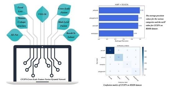
Figure 10 shows the mAP values of CF2PN in the DIOR dataset and RSOD dataset, respectively, as well as the average accuracy (AP) values of various categories on both datasets. As can be seen in DIOR dataset, there are 12 categories with AP values exceeding 0.7, namely, basketball court, tennis court, windmill, airplane, airport, ground track field, baseball field, ship, golf field, expressway service area, chimney and stadium. In addition, the AP values for dam, overpass, harbor, storage tank, expressway toll station and train station all exceed 0.5. In the RSOD dataset, the AP values for oil tanks, playgrounds and aircraft are above 0.95, and only the AP value for the overpass category is below 0.9.

However, the results of our model are not satisfactory for the two categories of vehicles and bridges in the DIOR dataset, namely, vehicles and bridges. There are two reasons for this result. First, the number of vehicles is more than any other objects, and the vehicles’ scenes are too complex. We used five feature layers for fusion in CSFM, which increases the contextual information provided by the scene. Second, samples from bridges have an inter-class similarity with samples from overpasses, which greatly increases the likelihood of misidentifying bridges as overpasses.

In addition, the reason why our method did not work very well in the RSOD dataset for detecting objects of the class overpass is due to the small number of training samples in the RSOD dataset. In Table 4, it can be seen that overpass is the class of objects with the lowest number of samples. Therefore, the improvement of the detection accuracy for small samples will also be included in our future research.

Figure 11 shows the confusion matrix detected by CF2PN in the DIOR dataset. The vertical coordinates of the matrix are the real labels and the horizontal coordinates are the prediction labels. The diagonal in the matrix is the number of samples of TP. In addition, the confusion matrix also shows that 57 bridge samples are predicted to be overpass, which also verifies the existence of interclass similarity between bridge and overpass.

Figure 12 shows the P_R curve of each class of target in the DIOR dataset. The larger the area of shaded part is, the better the algorithm effect will be. When bridge and vehicle have high accuracy, the recall rate is too low, resulting in poor detection effect.

As shown in Figure 13 and Figure 14, our proposed method achieved good results in the RSOD dataset.

4.2. Comparative Experiment

We executed multiple experiments on the DIOR dataset to confirm the effectiveness of our proposed CF2PN method. And our proposed CF2PN method produced the most advanced level of results with a mAP of 67.29%.

As shown in

Table 6. Comparison of the mAP values for different methods obtained for the DIOR dataset, where the results in bold represent the best performances. Each class corresponds to Table 5.

Detection Methods	Backbone	Class	Class	Class	Class	Class	Class	Class	Class	Class	Class	Class	Class	Class	Class	Class	Class	Class	Class	Class	Class	mAP (%)	F1 Score (%)
	Network	1	2	3	4	5	6	7	8	9	10	11	12	13	14	15	16	17	18	19	20
Faster RCNN [20]	ResNet-101	41.28	67.47	66.01	81.36	18.24	69.21	38.35	55.81	32.58	68.73	48.96	34.14	43.66	18.5	51.02	19.96	71.81	41.37	5.76	41.03	45.76	26.06
SSD [34]	VGG-16	82.55	54.79	78.76	88.92	35.75	74.39	52.02	71.39	58.67	52.21	74.9	44.52	49.59	78.35	69.32	60.12	89.92	38.23	39.54	82.46	63.82	40.58
RetinaNet [35]	ResNet-101	75.39	70.3	73.39	85.61	31.34	72.11	62.86	78.45	50.26	74.73	76.7	56.46	53.3	72.37	71.81	48.33	87.67	41.57	26.9	78.01	64.38	38.88
YOLOv3 [27]	Darknet53	66.98	79.71	78.39	85.89	39.64	72.44	70.69	85.65	65.01	74.61	79.83	44.97	58.93	33.67	59.61	34.58	89.14	61.72	37.88	79.16	64.93	44.49
YOLOV4-tiny [43]	CSPdarknet53-tiny	59.22	65.01	71.55	80.01	27.13	72.49	56.2	70.39	47.22	67.3	70.16	48.41	49.97	30.65	69.43	28.35	80.56	49.49	15.49	50.94	55.5	34.52
M2Det [42]	VGG-16	68.03	78.37	69.14	88.71	31.48	71.94	68.05	74.57	48.14	73.98	73.15	54.97	54.55	29.96	68.87	30.58	85.79	54.06	17.94	65.52	60.39	37.03
CF2PN	VGG-16	78.32	78.29	76.48	88.4	37	70.95	59.9	71.23	51.15	75.55	77.14	56.75	58.65	76.06	70.61	55.52	88.84	50.83	36.89	86.36	67.25	38.01

, the mAP value of Faster RCNN is the lowest, whereas the AP value for vehicles is only 5.76%. This is caused by the poor detection of small target objects by Faster RCNN on the one hand, and the lack of a good solution for targets with inter-class similarity by Faster RCNN on the other hand.

The mAP values of SSD, RetinaNet and YOLOv3 also all reached over 63%, because they all use multi-scale feature layers for prediction and obtain different size perceptual fields by different scale feature layers, thus improving the accuracy of detection. Additionally, M2Det also uses multi-scale feature layers for prediction where its network depth is too deep. Due to constant pooling operations, M2Det leads to the disappearance of shallow features used to detect small targets, thus reducing the performance. CF2PN aims at using M2DET to conduct cross-scale operation on the feature layer extracted from the backbone extraction network, to enrich its feature information.

The detection performance of M2Det is low in the DIOR dataset compared to that of the other detectors. This is due to the fact that the M2Det network only fuses the last two layers of the feature maps in the backbone extraction network, which greatly reduces the contextual semantic information. The reason why the performance of M2Det applied directly to remote sensing images is not significant is that the remote sensing image scenes are very complex. Therefore, the performance applied to remote sensing images is worse than that applied to natural images.

The CF2PN network detected more than 75% of the values for airplane, airport, baseball field, basketball court, golf field, ground track field, ship, tennis court, and wind mill. As can be seen, the proposed CF2PN method can detect not only large targets such as baseball fields and basketball courts, but also small targets, such as airplanes, ships and windmills.

Table 7. Comparison of the mAP values for different methods obtained for the RSOD dataset, where the results in bold represent the best performances.

Detection Methods	Backbone Network	Aircraft	Oil Tank	Overpass	Playground	mAP (%)	F1 Score (%)
Faster RCNN [20]	ResNet-101	50.20	98.12	95.45	99.31	85.77	77.00
SSD [34]	VGG-16	57.05	98.89	93.51	100.00	87.36	79.75
RetinaNet [35]	ResNet-101	75.01	99.23	54.68	94.66	80.90	75.75
YOLOv3 [27]	Darknet53	84.80	99.10	81.20	100.00	91.27	88.00
YOLOV4-tiny [43]	CSPdarknet53-tiny	66.47	99.42	80.68	99.31	86.47	82.25
M2Det [42]	VGG-16	80.99	99.98	79.10	100.00	90.02	80.50
CF2PN	VGG-16	95.52	99.42	83.82	95.68	93.61	89.25

shows the results of different algorithms on RSOD data. The proposed method shows advantages of small target detection such as aircrafts. Compared with YOLOv3, the AP value of our method increased by 10.72% for aircraft.

4.3. Ablation Experiments and Discussion

The contrast experiments were designed to evaluate the effectiveness of the proposed CF2PN, using the cross-scale feature fusion and focal loss function, respectively.

In

Table 8. Ablation study for the DIOR dataset, where the results in bold represent the best performances and the total parameters of each network.

Detection Methods	mAP(%)	F1 Score(%)	Parameters
M2Det	60.39	37.03	86.5M
M2Det + CSFM	57.76	35.16	86.2M
M2Det + focal loss	63.32	32.95	91.9M
CF2PN	67.25	38.01	91.6M

and

Table 9. Ablation study for the RSOD dataset, where the results in bold represent the best performances and the total parameters of each network.

Detection Methods	mAP (%)	F1 Score (%)	Parameters
M2Det	90.02	80.50	86.5M
M2Det + CSFM	87.30	76.75	86.2M
M2Det + focal loss	91.00	86.50	91.9M
CF2PN	93.61	89.25	91.6M

, the M2Det + CSFM method represents a fusion of five feature layers extracted from the VGG-16 backbone network, and its performance is lower than that of the M2Det approach. This is due to the fact that the fusion of the five feature layers enriches the scene with contextual information and adds a large amount of background, leading to an imbalance of positive and negative samples and an increase the error detection rate.

In Table 6, the average precision value of the ship in class 14 detected using the M2Det detector was 29.96%, while the AP value of the ship detected by our proposed CF2PN network reached 76.06%. This is due to the more complex background and rich semantic information of the image containing the ship. Therefore, we enhanced the semantic information by using CSFM and achieved balanced positive and negative samples via focal loss.

Several sets of experiments on the DIOR dataset were compared and analyzed to demonstrate that the proposed CF2PN method reaches the most advanced performance and that it demonstrates a superior performance in detecting multi-scale and complex objects. However, for some of the object classes in Table 6, such as bridge and vehicle, the detection accuracy is still very low, and it is difficult to achieve satisfactory results with the existing methods. This problem may be due to the relatively low image quality of these two types of scenes and their overly complex and cluttered backgrounds, which leads to objects being missed.

Thus, the accurate detection of objects in DIOR datasets with more complex scenarios remains a challenge. In future work, the more accurate detection of objects with complex scenarios will be the key goal.

5. Conclusions

Nowadays, the technology of optical remote sensing images with high resolution target detection is the focus of the majority of researchers, and a large number of optical remote sensing images target detection algorithms have appeared that have focused mainly on two-stage target detection methods based on Faster-RCNN and SSD one-stage target detection. However, both types of target detection algorithms for high-resolution remote sensing images face the following three problems: (1) there is great variability in objects sizes in remote sensing images with high resolution, and the ground objects vary in size even when they are in the same class; (2) since high-resolution remote sensing images are characterized by a large field of view (usually covering several square kilometers), a variety of backgrounds may be included in the field of view, which can interfere strongly with their object detectors; and (3) many of the objects in high-resolution remote sensing images are small (tens of, even a few, pixels), which leads to low object information. CNN-based target detection methods have achieved good results in traditional target detection datasets, but for small objects, further information reduction will be achieved by the CNN pooling layer, which ultimately makes low dimensions too difficult to identify.

For solving the above problems, CF2PN as a new object detector is proposed, which resolves the large size differences between objects in remote sensing images with high-resolution by means of feature fusion via multi-level and multi-scale methods. To address the problem of high background complexity in high-resolution remote sensing images, we balanced the positive and negative samples by using a focal loss function.

However, although the proposed method achieved the most advanced results, its performance for more complex scenes is still not satisfactory. In further work, we will address how to extract useful features from complex scene contextual information, and combine the natural language processing domain. In addition, remote sensing images may also appear hazy due to light, weather, and other factors. This is still a big challenge for the performance of the algorithm. Therefore, the detection of hazy images is also a direction of our future exploration.

References

- Hou, Y.; Zhu, W.; Wang, E. Hyperspectral Mineral Target Detection Based on Density Peak. Intell. Autom. Soft Comput. 2019, 25, 805–814. [Google Scholar] [CrossRef]
- Sun, L.; Wu, F.; He, C.; Zhan, T.; Liu, W.; Zhang, D. Weighted Collaborative Sparse and L1/2 Low-Rank Regularizations With Superpixel Segmentation for Hyperspectral Unmixing. IEEE Geosci. Remote Sens. Lett. 2020. [Google Scholar] [CrossRef]
- Papageorgiou, C.P.; Oren, M.; Poggio, T. A general framework for object detection. In Proceedings of the Sixth International Conference on Computer Vision, Bombay, India, 4–7 January 1998. [Google Scholar]
- Dalal, N.; Triggs, B. Histograms of oriented gradients for human detection. In Proceedings of the IEEE Computer Society Conference on Computer Vision and Pattern Recognition (CVPR), San Diego, CA, USA, 20–26 June 2005; pp. 886–893. [Google Scholar]
- Fu, L.; Li, Z.; Ye, Q. Learning Robust Discriminant Subspace Based on Joint L2,p- and L2,s-Norm Distance Metrics. IEEE Trans. Neural Netw. Learn. Syst. 2020. [Google Scholar] [CrossRef] [PubMed]
- Ye, Q.; Li, Z.; Fu, L.; Yang, W.; Yang, G. Nonpeaked Discriminant Analysis for Data Representation. IEEE Trans. Neural Netw. Learn. Syst. 2019, 30, 3818–3832. [Google Scholar] [CrossRef] [PubMed]
- Ye, Q.; Yang, J.; Liu, F.; Zhao, C.; Ye, N.; Yin, T. L1-Norm Distance Linear Discriminant Analysis Based on an Effective Iterative Algorithm. IEEE Trans. Circuits Syst. Video Technol. 2018, 28, 114–129. [Google Scholar] [CrossRef]
- Ye, Q.; Zhao, H.; Li, Z.; Yang, X.; Gao, S.; Yin, T.; Ye, N. L1-norm Distance Minimization Based Fast Robust Twin Support Vector k-plane clustering. IEEE Trans. Neural Netw. Learn. Syst. 2018, 29, 4494–4503. [Google Scholar] [CrossRef]
- Gunn, S.R. Support vector machines for classification and regression. ISIS Tech. Rep. 1998, 14, 5–16. [Google Scholar]
- Xu, F.; Zhang, X.; Xin, Z.; Yang, A. Investigation on the Chinese Text Sentiment Analysis Based on ConVolutional Neural Networks in Deep Learning. Comput. Mater. Contin. 2019, 58, 697–709. [Google Scholar] [CrossRef] [Green Version]
- Guo, Y.; Li, C.; Liu, Q. R2N: A Novel Deep Learning Architecture for Rain Removal from Single Image. Comput. Mater. Contin. 2019, 58, 829–843. [Google Scholar] [CrossRef] [Green Version]
- Wu, H.; Liu, Q.; Liu, X. A Review on Deep Learning Approaches to Image Classification and Object Segmentation. Comput. Mater. Contin. 2019, 60, 575–597. [Google Scholar] [CrossRef] [Green Version]
- Zhang, X.; Lu, W.; Li, F.; Peng, X.; Zhang, R. Deep Feature Fusion Model for Sentence Semantic Matching. Comput. Mater. Contin 2019, 61, 601–616. [Google Scholar] [CrossRef]
- Hung, C.; Mao, W.; Huang, H. Modified PSO Algorithm on Recurrent Fuzzy Neural Network for System Identification. Intell. Auto Soft Comput. 2019, 25, 329–341. [Google Scholar]
- Girshick, R.; Donahue, J.; Darrell, T.; Malik, J. Rich feature hierarchies for accurate target detection and semantic segmentation. In Proceedings of the IEEE Conference on Computer Vision and Pattern Recognition (CVPR), Columbus, OH, USA, 23–27 June 2014; pp. 580–587. [Google Scholar]
- Everingham, M.; VanGool, L.; Williams, C.K.I.; Winn, J.; Zisserman, A. The PASCAL Visual Object Classes (VOC) Challenge. IJCV 2010, 88, 303–338. [Google Scholar] [CrossRef] [Green Version]
- Li, X.; Shang, M.; Qin, H.; Chen, L. Fast Accurate Fish Detection and Recognition of Underwater Images with Fast R-CNN; IEEE: Piscataway, NJ, USA, 2015; pp. 921–925. [Google Scholar]
- Qian, R.; Liu, Q.; Yue, Y.; Coenen, F.; Zhang, B. Road Surface Traffic Sign Detection with Hybrid Region Proposal and Fast R-CNN; IEEE: Piscataway, NJ, USA, 2016; pp. 555–559. [Google Scholar]
- Wang, K.; Dong, Y.; Bai, H.; Zhao, Y.; Hu, K. Use Fast R-CNN and Cascade Structure for Face Detection; IEEE: Piscataway, NJ, USA, 2016; p. 4. [Google Scholar]
- Ren, S.; He, K.; Girshick, R.; Sun, J. Faster R-CNN: Towards Real-Time Target detection with Region Proposal Networks. In Advances in Neural Information Processing Systems; IEEE: Piscataway, NJ, USA, 2015; Volume 28. [Google Scholar]
- Mhalla, A.; Chateau, T.; Gazzah, S.; Ben Amara, N.E.; Assoc Comp, M. PhD Forum: Scene-Specific Pedestrian Detector Using Monte Carlo Framework and Faster R-CNN Deep Model; IEEE: Piscataway, NJ, USA, 2016; pp. 228–229. [Google Scholar]
- Zhai, M.; Liu, H.; Sun, F.; Zhang, Y. Ship Detection Based on Faster R-CNN Network in Optical Remote Sensing Images; Springer: Singapore, 2020; pp. 22–31. [Google Scholar]
- Redmon, J.; Divvala, S.; Girshick, R.; Farhadi, A. You Only Look Once: Unified, Real-Time Target detection. In Proceedings of the 2016 IEEE Conference on Computer Vision and Pattern Recognition, Las Vegas, NV, USA, 27–30 June 2016; pp. 779–788. [Google Scholar]
- Zhang, X.; Qiu, Z.; Huang, P.; Hu, J.; Luo, J. Application Research of YOLO v2 Combined with Color Identification. In Proceedings of the 2018 International Conference on Cyber-Enabled Distributed Computing and Knowledge Discovery, Zhengzhou, China, 18–20 October 2018; pp. 138–141. [Google Scholar]
- Itakura, K.; Hosoi, F. Automatic Tree Detection from Three-Dimensional Images Reconstructed from 360 degrees Spherical Camera Using YOLO v2. Remote Sens. 2020, 12, 988. [Google Scholar] [CrossRef] [Green Version]
- Bi, F.; Yang, J. Target Detection System Design and FPGA Implementation Based on YOLO v2 Algorithm; IEEE: Singapore, 2019; pp. 10–14. [Google Scholar]
- Redmon, J.; Ali, F. Yolov3: An incremental improvement. arXiv 2018, arXiv:1804.02767. [Google Scholar]
- Zhang, X.; Yang, W.; Tang, X.; Liu, J. A Fast Learning Method for Accurate and Robust Lane Detection Using Two-Stage Feature Extraction with YOLO v3. Sensors 2018, 18, 4308. [Google Scholar] [CrossRef] [Green Version]
- Adarsh, P.; Rathi, P.; Kumar, M. YOLO v3-Tiny: Target detection and Recognition Using One Stage Improved Model; IEEE: Piscataway, NJ, USA, 2020; pp. 687–694. [Google Scholar]
- Liu, G.; Nouaze, J.C.; Mbouembe, P.L.T.; Kim, J.H. YOLO-Tomato: A Robust Algorithm for Tomato Detection Based on YOLOv3. Sensors 2020, 20, 2145. [Google Scholar] [CrossRef] [PubMed] [Green Version]
- Liu, M.; Wang, X.; Zhou, A.; Fu, X.; Ma, Y.; Piao, C. UAV-YOLO: Small Object Detection on Unmanned Aerial Vehicle Perspective. Sensors 2020, 20, 2238. [Google Scholar] [CrossRef] [Green Version]
- Li, J.; Gu, J.; Huang, Z.; Wen, J. Application Research of Improved YOLO V3 Algorithm in PCB Electronic Component Detection. Appl. Sci. 2019, 9, 3750. [Google Scholar] [CrossRef] [Green Version]
- Huang, Z.; Wang, J. DC-SPP-YOLO: Dense connection and spatial pyramid pooling based YOLO for target detection. Inf. Sci. 2020, 522, 241–258. [Google Scholar] [CrossRef] [Green Version]
- Liu, W.; Anguelov, D.; Erhan, D.; Szegedy, C.; Fu, C.; Berg, A.C. SSD: Single Shot Multibox Detector. In Proceedings of the European Conference on Computer Vision, Amsterdam, The Netherlands, 8–16 October 2016; pp. 21–37. [Google Scholar]
- Lin, T.Y.; Goyal, P.; Girshick, R.; He, K.; Dollár, P. Focal loss for dense object detection. In Proceedings of the IEEE International Conference on Computer Vision (ICCV), Venice, Italy, 2–29 October 2017; pp. 2980–2988. [Google Scholar]
- Zhao, W.; Ma, W.; Jiao, L.; Chen, P.; Yang, S.; Hou, B. Multi-scale image block-level f-cnn for remote sensing images target detection. IEEE Access 2019, 7, 43607–43621. [Google Scholar] [CrossRef]
- Sergievskiy, N.; Ponamarev, A. Reduced focal loss: 1st place solution to xview target detection in satellite imagery. arXiv 2019, arXiv:1903.01347. [Google Scholar]
- Chen, C.; Gong, W.; Chen, Y.; Li, W. Target detection in remote sensing images based on a scene-contextual feature pyramid network. Remote Sensing 2019, 11, 339. [Google Scholar] [CrossRef] [Green Version]
- Yang, X.; Yang, J.; Yan, J.; Zhang, Y.; Zhang, T.; Guo, Z. SCRDet: Towards more robust detection for small, cluttered and rotated objects. In Proceedings of the IEEE International Conference on Computer Vision (ICCV), Seoul, Korea, 22 April 2019; pp. 8232–8241. [Google Scholar]
- Yang, X.; Yan, J.; Yang, X.; Tang, J.; Liao, W.; He, T. SCRDet++: Detecting small, cluttered and rotated objects via instance-level feature denoising and rotation loss smoothing. arXiv 2020, arXiv:2004.13316. [Google Scholar]
- Li, K.; Wan, G.; Cheng, G.; Meng, L.; Han, J. Target detection in optical remote sensing images: A survey and a new benchmark. ISPRS 2020, 159, 296–307. [Google Scholar]
- Zhao, Q.; Sheng, T.; Wang, Y.; Tang, Z.; Ling, H. M2det: A single-shot object detector based on multi-level feature pyramid network. In Proceedings of the AAAI Conference on Artificial Intelligence, Honolulu, HI, USA, 27 January–1 February 2019; Volume 33, pp. 9259–9266. [Google Scholar]
- Wang, C.Y.; Bochkovskiy, A.; Liao, H.Y.M. Scaled-YOLOv4: Scaling Cross Stage Partial Network. arXiv 2020, arXiv:2011.08036. [Google Scholar]
- Hu, J.; Shen, L.; Albanie, S.; Sun, G.; Wu, E. Squeeze-and-excitation networks. In Proceedings of the IEEE Conference on Computer Vision and Pattern Recognition, Honolulu, HI, USA, 21–26 July 2017; pp. 7132–7141. [Google Scholar]
- Sun, L.; Tang, Y.; Zhang, L. Rural Building Detection in High-Resolution Imagery Based on a Two-Stage CNN Model. IEEE Geosci. Remote Sens. Lett. 2017, 14, 1998–2002. [Google Scholar] [CrossRef]
- Cheng, G.; Zhou, P.; Han, J. Learning Rotation-Invariant Convolutional Neural Networks for Target detection in VHR Optical Remote Sensing Images. IEEE Geosci. Remote Sens. 2016, 54, 7405–7415. [Google Scholar] [CrossRef]
- Chen, C.Y.; Gong, W.G.; Hu, Y.; Chen, Y.L.; Ding, Y. Learning Oriented Region-based Convolutional Neural Networks for Building Detection in Satellite Remote Sensing Images. Int. Arch. Photogramm. Remote Sens. Spat. Inf. Sci. 2017, XLII-1/W1, 461–464. [Google Scholar] [CrossRef] [Green Version]
- Deng, Z.; Sun, H.; Zhou, S.; Zhao, J.; Lei, L.; Zou, H. Multi-scale target detection in remote sensing imagery with convolutional neural networks. ISPRS J. Photogramm. Remote Sens. 2018, 145, 3–22. [Google Scholar] [CrossRef]
- Yang, X.; Sun, H.; Fu, K.; Yang, J.; Sun, X.; Yan, M.; Guo, Z. Automatic Ship Detection in Remote Sensing Images from Google Earth of Complex Scenes Based on Multiscale Rotation Dense Feature Pyramid Networks. Remote Sens. 2018, 10, 132. [Google Scholar] [CrossRef] [Green Version]
- Gao, X.; Sun, X.; Zhang, Y.; Yan, M.; Xu, G.; Sun, X.; Jiao, J.; Fu, K. An end-to-end neural network for road extraction from remote sensing imagery by multiple feature pyramid network. IEEE Access. 2018, 6, 39401–39414. [Google Scholar] [CrossRef]
Figure 1.
Inter-class similarity as shown in (a,b), intra-class variability as shown in (c,d).
Figure 2.
The CF2PN architecture.
Figure 3.
Convolution kernel substitution module.
Figure 4.
CSFM: cross-scale fusion module.
Figure 5.
Single TUM module.
Figure 6.
FFM2 module. This module is used to merge base features with the TUM.
Figure 7.
SFAM.
Figure 8.
DIOR dataset.
Figure 9.
Visualization results for the CF2PN on the DIOR dataset in (a–l); visualization results for the CF2PN on the RSOD dataset in (m–p).
Figure 10.
The average precision (AP) values for the various categories and the mAP value for CF2PN in the DIOR dataset and RSOD dataset as shown in (a,b), respectively.
Figure 11.
Confusion matrix of CF2PN on DIOR dataset. The index of each category is shown in Table 5.
Figure 12.
P-R curves of CF2PN for each category on the DIOR dataset, where the horizontal axis represents the recall for each class of target and the vertical axis represents the precision for each class of target and the scale is the normalized probability.
Figure 13.
Confusion matrix of CF2PN on RSOD dataset.
Figure 14.
P-R curves of CF2PN for each category on the RSOD dataset, where the horizontal axis represents the recall for each class of target and the vertical axis represents the precision for each class of target and the scale is the normalized probability.