Implementation of an Improved Water Change Tracking (IWCT) Algorithm: Monitoring the Water Changes in Tianjin over 1984–2019 Using Landsat Time-Series Data

Abstract

Tianjin is the largest open city along the coastline in Northern China, which has several important wetland ecosystems. However, no systematic study has assessed the water body changes over the past few decades for Tianjin, not to mention their response to human activities and climate change. Here, based on the water change tracking (WCT) algorithm, we proposed an improved water change tracking (IWCT) algorithm, which could remove built-up shade noise (account for 0.4%~6.0% of the final water area) and correct omitted water pixels (account for 1.1%~5.1% of the final water area) by taking the time-series data into consideration. The seasonal water product of the Global Surface Water Data (GSWD) was used to provide a comparison with the IWCT results. Significant changes in water bodies of the selected area in Tianjin were revealed from the time-series water maps. The permanent water area of Tianjin decreased 282.5 km² from 1984 to 2019. Each time after the dried-up period, due to government policies, the land reclamation happened in Tuanbo Birds Nature Reserve (TBNR), and, finally, 12.6 km² of the lake has been reclaimed. Meanwhile, 488.6 km² of land has been reclaimed from the sea along the coastal zone in the past 16 years at a speed of 28.74 km² yr⁻¹ in the Binhai New Area (BHNA). The method developed in this study could be extended to other sensors which have similar band settings with Landsat; the products acquired in this study could provide fundamental reference for the wetland management in Tianjin.

1. Introduction

Inland water systems often provide critical ecosystem functions, i.e., water and food provision, local climate regulation, conservation of biological diversity [1,2,3]. However, due to intensive human activities (e.g., land reclamation and water conservancy projects), the area of inland water decreased sharply in China [4,5]. Thus, accurate monitoring the long-term changes of inland water bodies is important to both scientific community for water research and local governments for water-resource planning and management [6,7,8,9,10,11].

Remote sensing has become one of the most efficient methods in water area monitoring with synoptic and repeated observations. Various methods have been developed to discriminate and map water using multi-spectral, hyperspectral and radar images [12,13,14]. The most simple and popular method was basis on threshold segmentation by using a single band, or a ratio of two bands of data (e.g., Normalized Difference Vegetation Index (NDVI), Normalized Difference Water Index (NDWI) [15] and the Modified Normalized Difference Water Index (MNDWI) [16,17]). However, as the spectral characteristics of lakes vary temporally and spatially, the single threshold may not be suitable for large areas and long time-interval due to varied band configurations and illumination conditions [14]. The supervised classification, decision tree and machine learning algorithms were also used to classify the water body [18,19], while they need training data from different regions and different seasons to serve as prior knowledge or auxiliary data.

The daily global water map data set from 2001 to 2016 was generated based on 500-m resolution time-series daily MODIS (Moderate Resolution Imaging Spectroradiometer) reflectance data [20,21]. The MODIS 250-m resolution data collected between 2000 and 2010 were used by Feng et al. [13] to document the temporal inundation changes of Poyang Lake with Floating Algae Index (FAI) and a gradient method. Han and Niu [21] constructed a new Global Surface Water Extent Dataset (GSWED) covering 2000–2018 with a temporal resolution of 8 days and a spatial resolution of 250 m based on MODIS data and Google Earth Engine (GEE) cloud computing platform. Although, the 250-m and 500-m resolution MODIS data can be used to effectively analyze the long-term water body changes in large areas, the results obtained from the MODIS images may misinterpret the small-scale inland water bodies due to a mixing pixels problem [22]. The publicly accessible Landsat archive makes the historical water body mapping feasible at 30-m level [23]. Based on classification tree models and top of atmosphere (TOA) reflectance of 3.4 million Landsat scenes, Pickens et al. [19] generated the global water maps and assessed the accuracy using sub-pixel analysis based on samples from 5-m resolution RapidEye imagery. Hou, et al. [24] delineated the lake boundaries using a thresholding method based on Landsat-derived NDWI to track reclamation-induced changes in the Yangtze Plain lakes. The Function of mask (FMASK) was developed to detect cloud, cloud shadow, water and snow for time-series Landsat images [25,26]. With Landsat time-series, the global inland water dynamic was documented by different methods (multiple indices and thresholds, the expert system based on a procedural sequential decision tree, etc.) [19,27,28]. The multi-source remote sensing data were also used for small-coverage inland water detection [29,30,31,32]. These methods need a large number of auxiliary data and thus cannot be fully automated employed to extract long-term water areas.

Recently, a water change tracking (WCT) algorithm based on Minimum Normalized Water Score (MNWS) for accurate inland water mapping was proposed and has been proven to be a promising method for Landsat images to extract water bodies automatically. Compared with FMASK and G1WBM methods, the WCT algorithm seems to be more robust for inland water extraction. However, while the WCT algorithm has been validated on large lakes, non-urban areas and wetland water extraction in China, its ability for small lakes and urban-dominated area water extraction has not been discussed. When this method was applied to extract water bodies in urban-dominant area in Tianjin, lots of very bright water pixels were omitted and the algorithm performed poorly in urban areas with high buildings. Hence, given the availability of the time-series Landsat images and lack of systematic assessment of the Tianjin water bodies, this study has two objectives:

(1)

Improve the existing WCT algorithm to extract the water bodies in Tianjin using Landsat images;

(2)

Document water changes in Tianjin over 1984–2019 and understand their linkage with human activities and climate changes.

The IWCT can remove the built-up shades and correct the omitted pixels using the time-series remote sensing data. Furthermore, the IWCT will be fully validated in the urban dominated areas.

2. Materials and Methods

2.1. Study Area

Tianjin, located at the downstream of Haihe river Basin (116°42′7.5″–118°3′37.6″E and 38°33′23″–40°15′7.5″N, Figure 1), is the largest open city along the coastline in northern China. Influenced by temperate monsoon climate, Tianjin has two seasons: dry season (September to June) and wet season (July to August), and more than 60% of annual precipitation occurs in the wet season [33]. The wetland resources in Tianjin serve as the main resting places for migratory birds from East Asia to Australia. To conserve the rare and endangered migratory birds, the government has constructed several nature reserves: Beidagang Wetland Nature Reserve (BWNR), Dahuangpu Wetland Nature Reserve (DWNR), Ancient Coast and Wetland National Nature Reserve (ACWNNR) and Tuanbo Birds Nature Reserve (TBNR). The other major water bodies of Tianjin distributed in the Yuqiao Reservoir (YR) which is the important source of drinking water for Tianjin, and Binhai New Area (BHNA).

2.2. Dataset

Landsat surface reflectance data, including Landsat 8 Operational Land Imager (OLI), Landsat 7 Enhanced Thematic Mapper Plus (ETM+), Landsat 5 Thematic Mapper (TM) and Landsat 4 Thematic Mapper (TM) with 30-m resolution were downloaded from the U.S. Geological Survey (USGS) (http://glovis.usgs.gov/) and used to map Tianjin water bodies and their spaito-temporal changes. The entire study region is covered by four Landsat footprints (path 122 row 032, path 122 row 033, path 123 row 032 and path 123 row 033). After excluding images with significant cloud covers based on visual inspection, 1087 Landsat images between 1984 and 2019 were kept. The temporal distribution of the data is shown in the bubble chart (Figure 2). The size of the bubbles represents the valid observation area after removing the “bad pixels” (snow, ice or cloud covered areas in the satellite images), and arranges from small (the smallest valid observation area, 500 km²) gradually to large (the largest valid observation area, 13,000 km²).

The high-resolution images on Google Earth could be used as ground truth for the water classification. Two high-resolution images (acquisition on 21 November 2005 and 27 May 2018) that 1 day ahead and on the same day with the objective Landsat images (20051122123LE07 and 20180527122LE07) were used to discriminate the water and non-water pixels. The seasonality dataset of Global Surface Water-Data (GSWD) for Tianjin was downloaded from the website (https://global-surface-water.appspot.com/) [3]. The Seasonality map provides the intra-annual changes of water surface in the period of October 2014 to October 2015 and shows the number of months water was present. The images were used to select ground truth water samples to validate the Landsat extract water maps. The Shuttle Radar Topography Mission (SRTM) DEM data of Tianjin were downloaded from USGS. The urban boundary was downloaded from the website (http://data.ess.tsinghua.edu.cn/) [34]. The GaoFen (GF)-2 PMS data were downloaded from China Centre for Resources Satellite Data and Application (http://www.cresda.com/CN/). Precipitation and temperature data were obtained from the three meteorological stations (Baodi, Tianjin and Tanggu, shown in Figure 1) through China Meteorological Data Service Center (CMDC) (http://data.cma.cn/en).

Furthermore, the boundary of YR used in this study was calculated based on the largest inundation of YR during the whole study period. The boundary of four nature reserves and BHNA was obtained from Tianjin Institute of Surveying and Mapping (http://tjch.com.cn/).

2.3. Method

The WCT algorithm is designed to automatically extract multi-temporal water maps for large area. The processing steps could be summarized as follows:

• Collection of Reliable Water Samples (RWS): The RWS was extracted by the criteria that MNDWI was larger than 0.3 and the minimum reflectance of the red, green, and near infrared bands (MGRN) lower than 0.15 [27,35].
• Water sample clustering for the Reliable Water Samples: The k-means clustering method was applied to the visible bands of the RWS to cluster the water bodies into eight classes. The spectral statistical parameters (the mean and standard deviation values) for each band of each cluster were calculated.
• Calculation of the Minimum Normalized Water Score (MNWS): The Normalized Water Score (NWS) were calculated for all the images and the MNWS was calculated by the Equations (1) and (2).

  $$NW{S}_i=\sqrt{\frac{1}{m}{\displaystyle \sum _{j=1}^m{\left(\frac{\left(x_j-\overline{x_{i,j}}\right)}{{\sigma }_{i,j}}\right)}^2}},$$

  (1)

  $$MNWS={\min }_{i=1}^n\left\{NW{S}_i\right\},$$

  (2)

  $\overline{x_{i,j}}$ and ${\sigma }_{i,j}$ is the mean and standard deviation of cluster $i$ and band $j$,$m$ is the number of the band, $n$ is the number of the cluster.
• Extraction of Water Body: The water body extracted by the criteria that the MNWS < 2.5.

When applied the WCT algorithm to the study region for the Landsat time-series images of 1984–2019, we found that the WCT algorithm has some defects. The defects of the WCT could be summarized as follows:

(1)

Water pixels with very high reflectance may be misclassified as background. The k-means clustering method was applied to the RWS to divide water bodies into different clusters according to the local environment. The WCT is highly dependent on the RWS selected from the images. The water pixels in the sun glint and in shallow areas affected by sand bottoms may be observed as high reflectance data. The water samples of these regions always did not meet the criteria of RWS and would be misclassified to non-water pixels.

(2)

Urban building shadows may be misclassified as water. The built-up shade noise account for 0.4%~6.0% of the final water areas from June to December/next January. The spectral characteristics of the materials under the shadows were not represented and the shadows share similar spectral characters with water. If the shadows in the images were not masked, they may be misinterpreted as water.

(3)

The time-series data were used to detect the changes of the water in the WCT algorithm, rather than extracting water. The omitted water pixels account for 1.1%~5.1% of the final water areas.

Based on the WCT algorithm, we proposed an improved water change tracking (IWCT) algorithm to overcome the defects of the WCT. The flow chart (Figure 3) shows the details of the data processing steps. The practical processing steps show as follows:

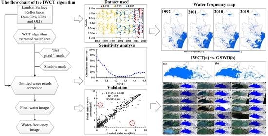
• The WCT algorithm: Implied the WCT algorithm described in the Section 2.3 to the Landsat (TM/ETM+ and OLI) images to extract preliminary water body map [12].
• “Bad pixel” mask: When the water pixel is covered by snow, cloud or ice, the spectral characteristic of the pixel changes greatly. The automatic cloud detection methods may be not suitable in this study because of their limits, such as ① The ground objects with high reflectance may be misclassified as clouds; ② It is hard to determine the boundary of optically thin clouds and their shadows; ③ Water may be misclassified to cloud shadows. In this study, visual interpretation method was used to remove bad pixels. Red-Green-Blue “true-color” composite images were generated using three bands (Red Band: 655, Green Band: 536, Blue Band: 480 nm) from the Landsat data. The regions where the RGB images showed “bad pixels” were manually delineated using the region of interest (ROI) Tool. The pixels within the ROI will be set as non-valid observations and discarded.
• Shadow mask: The spectral characteristics of the terrain and building shadows are similar to water and are always misinterpreted as water in the original algorithms. The water bodies and terrain shadows could be separated using the DEM data with the criteria that if the slopes of the pixels are greater than 5° [27]. In the urban-dominated areas, the shadows of high buildings will affect the water extraction accuracy. Building shadows is seasonally dependent, and will be related to the changes in the solar angle. When the sun is directly over the Tropic of Cancer on 21 June of the year, the sun has highest elevation angle in the northern hemisphere. Considering the geographic coordinates of Tianjin area, the images collected in June–July were less affected by the urban shade, and thus can be used to distinguish urban shades in the urban areas delineated by the urban boundary and water bodies for the rest data of the year.
• Omitted water pixels correction: Using only one index combination often leads to omission errors for those water pixels with high reflectance. With the repeat monitoring, the remote sensing not only provides spatial information, it also provides the temporal coverage of water bodies. Thus, the time-series water classification results and Landsat reflectance data were used to correct the water pixels which were omitted in the WCT algorithm. Images in the same month within a four-year window (i.e., two years before and later) were selected, if the data were classified as water within four years, and the data meet the criteria (MNDWI > 0 or NDWI > 0 or NDVI < 0 and NDVI < 0.3) it will set as omitted water.
• Water frequency and water area mapping: For each pixel, the water frequency map is calculated as the ratio of the number of pixels detected as water and the number of valid observations within one year. To quantify the water area changes of Tianjin during the last three decades, the water areas of the six typical regions (ACWNNR, BWNR, DWNR, TBNR, BHNA and YR) were calculated for all the cloud-free Landsat images of these specific regions. Pixels with water frequency equals 1 were classified as permanent water.

2.4. Accuracy Assessment

The omission and commission errors at pixel scale were used to evaluate the performance of the IWCT. For the selected two Landsat images, 2000 random points for water and non-water pixels in the IWCT images were generated within the overlapped region between Google earth high-resolution images and Landsat data (20051122123LE07 and 20180527122LE07). The points were visually classified as water/non-water on the Google Earth high-resolution image, and were used for validation of the result.

As both of the seasonal GSWD products and IWCT-based water map were calculated with the entire archive of the Landsat images and have the same spatial resolution, the GSWD product can be used to assess the accuracy of IWCT-based results. The seasonality map of the water surfaces for a single year (2014–2015) was available on the website, and was chosen to make a comparison with the data calculated in this study. If all the pixels in the valid observations are water pixels, the data will be marked as permanent water in the GSWD. As the water frequency was calculated based on the ratio between the number of pixels detected as water and the number of valid observations, the pixels with water frequency equal to 1 would be treated as permanent water for IWCT. The permanent water in the GSWD and the permanent water in IWCT were calculated based on the same principle. The permanent water data of the two images were resampled to the same resolution as 3 km × 3 km, and then the correlation analysis was conducted for all the points in the data. To test the applicability of proposed algorithm, it was applied to a FLAASH atmospheric corrected GF-2 PMS image. The extraction result based on 3.9-m resolution GF-2 PMS was then compared with Landsat result.

3. Results

The water bodies were extracted using the IWCT method excluding the bad pixels and shadows. The omitted water pixels were corrected using the time-series Landsat images and primary water results. To assess the accuracy of IWCT product, the commission and omission errors of the WCT and IWCT were estimated using the same validation samples. The results show that the IWCT method was much better than the WCT by providing lower commission errors and omission errors (

Table 1. Classification accuracy of the WCT and IWCT.

	WCT		IWCT
Image	Commission Error	Omission Error	Commission Error	Omission Error
20051122123LE07	9.5%	4.3%	5.1%	3.2%
20180527122LE07	0.8%	2.4%	0.8%	0.9%

). The IWCT presented lower commission and omission errors for 20051122123LE07 and 20180527122LE07 images than WCT algorithm (commission error: 0.8–5.1% for IWCT versus 0.8–9.5% for WCT, omission error: 0.9–3.2% for IWCT versus 2.4–4.3% for WCT). Scatterplots of permanent water area from IWCT, corresponding to 3 km × 3 km resolution, were made against GSWD. The result indicated that the two data have extremely high consistency with a determination coefficient (R²) of 0.97 and RMSE of 0.46 (p < 0.05) (Figure 4).

Figure 5 shows the dynamic water body maps of Tianjin between 1984 and 2019. Each map was generated using the Landsat time-series images in the corresponding year. The water bodies with higher frequencies are presented in dark blue and seasonal water with lower frequencies are shown in lighter blue. The spatial distributions of the water bodies were clearly demonstrated within each panel, and the long-term water frequency changes were also revealed across each panel. In general, the water bodies with high frequencies located mainly in the BHNA, YR and TBNR. The water frequencies are more variable in the ACWNNR, BWNR and DWNR in different years. The water landscape shows the trend of fragmentation from 1984 to 2019. The water area of TBNR shows significant variability in different years, with a larger area of water has been reclaimed in after 2002. In addition, land has been reclaimed from sea along the coastal zone after 2003 in the BHNA.

To present the details of the water changes in Tianjin, six typical regions were selected from Tianjin to show the long-term changes of water area. Figure 6 plots the estimated areas of water and permanent water bodies between 1984 and 2019, Figure 6a–g represent the results of ACWNNR, BWNR, DWNR, TBNR, BHNA, YR and Tianjin, respectively. All the cloud-free images in the corresponding area were considered when calculating the long-term changes. The coverages of the water area showed a seasonal and annual fluctuation trend during 1984–2019 for the ACWNNR, BWNR and DWNR (Figure 6a–c). The water area within TBNR showed a remarkable seasonal and annual fluctuation from 1984 to 2019, which almost dried up in the periods (1992–1994, 1999–2004, and 2008–2011) and remained at a fluctuated level (46.2~54.6 km²) after 2012 (Figure 6d). Specifically, the water area showed a fluctuation trend in the period (1984–2003) and a significant shrinking trend (−28.7 km² yr⁻¹, p < 0.05) after 2003 for the BHNA (Figure 6e). The water area of YR had a significant seasonal variation (Figure 6f). The permanent water area (including permanent shallow marine water and inland water) of Tianjin decreased 282.5 km² from 1984 to 2019.

4. Discussion

4.1. Driving Forces

To test whether the area of water bodies was driven by precipitation, the relationship between water area in each selected study area and local precipitation from the nearest meteorological station was examined. Correlation analysis showed a statistically significant correlation between the total precipitation of three months before the image acquisition dates and water area during July to September for four out of six sites, with the determination coefficients (R²) of 0.25 (N = 35, p < 0.01) for the BWNR, 0.07 (N = 71, p < 0.05) for DWNR, 0.16 (N = 72, p < 0.01) for TBNR and 0.29 (N = 61, p < 0.01) for YR, which are statistically significant. Specifically, the water area of the BHNA and precipitation showed a statistically significant correlation (R² = 0.71, p < 0.01) if the result in 1984 (red circled points) was not considered due to very low sea level in 1984. Note that the red data points in the TBNR and BHNA were collected after the land reclamation activities happened in the local study area, were not taken into consideration when making the correlation analysis (Figure 7). The precipitation appears to negatively correlate with the water area in ACWNNR (R² = 0.04, p > 0.05) and DWNR (R² = 0.07, p < 0.05). After checking the land use map, we found that the main vegetation types are dry land crop and paddy field crop for ACWNNR and DWNR, respectively (http://www.dsac.cn/DataProduct/Detail/20081103). The water bodies could be affected by the surface vegetation types. Thus, the changes in local precipitation might be partially associated to water area changes in July to September for parts of study regions.

The long-term change of water area or water quality could be taken as the indicators characterizing the ecosystem change. With historical surface water changing trends and ancillary data, we can document the impact of the human activities and climate change on the ecosystem. The water bodies of TBNR was considerably fluctuated in different years and remained at a low coverage level during the periods (1992–1994, 1999–2004, 2008–2011) (Figure 6d and Figure 8d,h,l) cloud be linked to important government policies. The reservoir was built in 1978, the storage capacity of the reservoir was 0.98 hundred million m³. The running out of water happened in 1992 is due to a project which increased the storage capacity of the reservoir (Figure 8c). The dike of the reservoir faced some safety problem after operation for a long time, the reservoir was repaired and carefully maintained after 2008 (http://www.docin.com/p-525234617.html); thus, the water ran out after 2008 (Figure 8k). Each time after the running out of water period, parts of the water area were reclaimed (Figure 8e,i,m) and finally 12.6 km² lake has been reclaimed. The decreasing of the water area after 2003 in the BHNA was attributed to the sea reclamation activities (Figure 9) [36]. Figure 9 showed the coastal line of the Tianjin in 2004, 2009, 2014 and 2019, indicating the land expanded towards sea, with an average trend of 28.7 km² yr⁻¹ from 2004 to 2019. The decrease of permanent water area in Tianjin was obtained in accordance with the decrease of permanent water area in BHNA. The permanent shallow marine waters gradually reduced due to sea reclamation activities in the BHNA after 2004. The permanent inland water areas fluctuated in different years. The decrease of permanent water area (including permanent shallow marine water and inland water) in Tianjin was due to sea reclamation activities.

Additionally, changes in other meteorological factors (i.e., temperature) might influence the evapotranspiration of water and thus the water coverage, no significant relationship was found between the temperature and water area over the six study regions.

4.2. Validity of the Results and Future Applications

Long-term changes of water in Tianjin were clearly revealed and quantified via Landsat observation. However, are these Landsat derived water areas valid?

IWCT method achieved much better performance than the WCT by providing lower commission errors and omission errors. The correlation analysis between the maximum water frequency maps from IWCT result (a) and GSWD result shows the two results are highly consistent except for several points (Figure 4). The red circled points located in the YR (Figure 10) show great difference were analyzed. There is a big difference for the water map between IWCT result (Figure 10a) and GSWD result (Figure 10b) for the two points (Figure 4). After inspecting all the water classification results and the corresponding RGB images from October 2014 to October 2015, we found that the IWCT-based water frequency map is more reliable. Although lots of cloud mask algorithms had been developed before, the algorithms still have issues that cannot be ignored for the time-series images and will induce uncertainties to the final water map [26]. After a more robust cloud mask algorithm was developed in the further, the algorithm will be used to automatically extract water map.

Several points classified as omitted water were used to carry out the sensitivity analysis in this study. We kept the criteria (MNDWI > 0 or NDWI > 0 or NDVI < 0) stable, and then changed the NDVI values from 0 to 0.5. The sensitivity analysis results can reflect the impact of different NDVI criteria on the omitted water detection. Results show that the classification error rate decreases with the increasing NDVI values, but increases as the NDVI > 0.3. The reason is that when NDVI > 0.3, the vegetation will be more probably misclassified as omitted water (Figure 11). Overall, the criteria (NDVI < 0.3) give satisfied results in the sensitivity analysis section.

The Chinese government has launched a series of high-resolution (GF) mapping satellites in the last seven years. The sensors onboard have similar spectral bands with the Landsat images and higher resolutions. We applied the proposed algorithm to 3.9-m resolution GF-2 PMS data which were collected on 29 May 2019 and on the same day as the OLI image. The water bodies for the two images were upscaled to 0.015° latitude and 0.007° longitude, respectively (Figure 12). A comparison showed that the water bodies extracted from GF-2 is consistent with the OLI-based result. The result shows that the algorithm can be used for GF-2 image water extraction and the high-resolution GF-2 image could be used to extract more small area of water (narrow rivers, small lakes).

5. Conclusions

In this study, we developed the IWCT method which could remove built-up shade noise and correct omitted water pixels by taking the time-series data into consideration. The algorithm shows better performance in the urban dominated areas. With the IWCT algorithm, we documented the time-series water body changes of Tianjin using observations during 1984–2019. The annual water frequency map shows significantly decreasing trends after the land reclaimed activities. In addition, 488.6 km² of land has been reclaimed from the sea along the coastal zone in the last 16 years at the speed of 28.74 km² yr⁻¹ in the BHNA. Overall, the change of water bodies in July to September could be partly attributed to precipitation except for the dry land crop and paddy field crop dominated areas, and the decrease of the water coverage appears to be a result of human activities.

IWCT method achieved much better performance than the WCT by providing lower commission and omission errors. However, this study still has some limitations. Although the urban boundary has been used to correct the IWCT algorithm in urban-dominated areas, parts of the urban shades (account for 2.9% of the randomly selected water pixels in the validation) were still misclassified as water. In the summer, the shadow of the skyscraper was misclassified as water. Very dark surface (the ground covered by coal, account for 0.1% of the randomly selected water pixels in the validation) will be misclassified as water. A more robust urban shade detection model is needed in the further research to remove the urban shades. The inclusion of manual clouds removal in the algorithm seriously limits its automatic application in large-scale dynamic inland water mapping. After developing a more robust cloud mask algorithm, the algorithm will be used to automatically extract water map. As several high-resolution sensors share similar bands with Landsat data, the method developed in this study can be extended to other sensors to study the long-term changes of even smaller water bodies in response to human activities and climate variability.

References

1. Sheng, Y.; Song, C.; Wang, J.; Lyons, E.A.; Knox, B.R.; Cox, J.S.; Gao, F. Representative lake water extent mapping at continental scales using multi-temporal Landsat-8 imagery. Remote Sens. Environ. 2016, 185, 129–141. [Google Scholar] [CrossRef] [Green Version]
2. Palmer, S.C.J.; Kutser, T.; Hunter, P.D. Remote sensing of inland waters: Challenges, progress and future directions. Remote Sens. Environ. 2015, 157, 1–8. [Google Scholar] [CrossRef] [Green Version]
3. Pekel, J.; Cottam, A.; Gorelick, N.; Belward, A.S. High-resolution mapping of global surface water and its long-term changes. Nature 2016, 540, 418–422. [Google Scholar] [CrossRef] [PubMed]
4. Ma, R.; Duan, H.; Hu, C.; Feng, X.; Li, A.; Ju, W.; Jiang, J.; Yang, G. A half-century of changes in China’s lakes: Global warming or human influence? Geophys. Res. Lett. 2010, 37. [Google Scholar] [CrossRef]
5. Gong, P.; Niu, Z.; Cheng, X.; Zhao, K.; Zhou, D.; Guo, J.; Liang, L.; Wang, X.; Li, D.; Huang, H.; et al. China’s wetland change (1990–2000) determined by remote sensing. Sci. China-Earth Sci. 2010, 53, 1036–1042. [Google Scholar]
6. Piao, S.; Ciais, P.; Huang, Y.; Shen, Z.; Peng, S.; Li, J.; Zhou, L.; Liu, H.; Ma, Y.; Ding, Y. The impacts of climate change on water resources and agriculture in China. Nature 2010, 467, 43–51. [Google Scholar] [CrossRef]
7. Oki, T.; Kanae, S. Global Hydrological Cycles and World Water Resources. Science 2006, 313, 1068–1072. [Google Scholar] [CrossRef] [Green Version]
8. Duan, W.; Zou, S.; Chen, Y.; Nover, D.; Fang, G.; Wang, Y. Sustainable water management for cross-border resources: The Balkhash Lake Basin of Central Asia, 1931–2015. J. Clean. Prod. 2020, 263, 121614. [Google Scholar] [CrossRef]
9. Duan, W.; Chen, Y.; Zou, S.; Nover, D. Managing the water-climate-food nexus for sustainable development in Turkmenistan. J. Clean. Prod. 2019, 220, 212–224. [Google Scholar] [CrossRef]
10. Liu, D.; Chen, W.; Menz, G.; Dubovyk, O. Development of integrated wetland change detection approach: In case of Erdos Larus Relictus National Nature Reserve, China. Sci. Total Environ. 2020, 731, 139166. [Google Scholar] [CrossRef]
11. Chen, W.; Cao, C.; Liu, D.; Tian, R.; Wu, C.; Wang, Y.; Qian, Y.; Ma, G.; Bao, D. An evaluating system for wetland ecological health: Case study on nineteen major wetlands in Beijing-Tianjin-Hebei region, China. Sci. Total Environ. 2019, 666, 1080–1088. [Google Scholar] [CrossRef] [PubMed]
12. Chen, X.; Liu, L.; Zhang, X.; Xie, S.; Lei, L. A Novel Water Change Tracking Algorithm for Dynamic Mapping of Inland Water Using Time-Series Remote Sensing Imagery. IEEE J. Sel. Top. Appl. Earth Obs. Remote Sens. 2020, 13, 1661–1674. [Google Scholar] [CrossRef]
13. Feng, L.; Hu, C.; Chen, X.; Cai, X.; Tian, L.; Gan, W. Assessment of inundation changes of Poyang Lake using MODIS observations between 2000 and 2010. Remote Sens. Environ. 2012, 121, 80–92. [Google Scholar] [CrossRef]
14. Khandelwal, A.; Karpatne, A.; Marlier, M.E.; Kim, J.; Lettenmaier, D.P.; Kumar, V. An approach for global monitoring of surface water extent variations in reservoirs using MODIS data. Remote Sens. Environ. 2017, 202, 113–128. [Google Scholar] [CrossRef]
15. McFeeters, S.K. The use of the Normalized Difference Water Index (NDWI) in the delineation of open water features. Int. J. Remote Sens. 1996, 17, 1425–1432. [Google Scholar] [CrossRef]
16. Xu, H. Modification of normalised difference water index (NDWI) to enhance open water features in remotely sensed imagery. Int. J. Remote Sens. 2006, 27, 3025–3033. [Google Scholar] [CrossRef]
17. Huang, W.; Duan, W.; Nover, D.; Sahu, N.; Chen, Y. An integrated assessment of surface water dynamics in the Irtysh River Basin during 1990–2019 and exploratory factor analyses. J. Hydrol. 2021, 593, 125905. [Google Scholar] [CrossRef]
18. Wang, S.; Zhang, L.; Zhang, H.; Han, X.; Zhang, L. Spatial–Temporal Wetland Landcover Changes of Poyang Lake Derived from Landsat and HJ-1A/B Data in the Dry Season from 1973–2019. Remote Sens. 2020, 12, 1595. [Google Scholar] [CrossRef]
19. Pickens, A.H.; Hansen, M.C.; Hancher, M.; Stehman, S.V.; Tyukavina, A.; Potapov, P.; Marroquin, B.; Sherani, Z. Mapping and sampling to characterize global inland water dynamics from 1999 to 2018 with full Landsat time-series. Remote Sens. Environ. 2020, 243, 111792. [Google Scholar] [CrossRef]
20. Ji, L.; Gong, P.; Wang, J.; Shi, J.; Zhu, Z. Construction of the 500-m resolution daily global surface water change database (2001–2016). Water Resour. Res. 2018, 54, 10–270. [Google Scholar] [CrossRef]
21. Han, Q.; Niu, Z. Construction of the Long-Term Global Surface Water Extent Dataset Based on Water-NDVI Spatio-Temporal Parameter Set. Remote Sens. 2020, 12, 2675. [Google Scholar] [CrossRef]
22. Carroll, M.L.; Townshend, J.R.G.; Dimiceli, C.; Noojipady, P.; Sohlberg, R.A. A new global raster water mask at 250 m resolution. Int. J. Digit. Earth 2009, 2, 291–308. [Google Scholar] [CrossRef]
23. Zhu, Z.; Wulder, M.A.; Roy, D.P.; Woodcock, C.E.; Hansen, M.C.; Radeloff, V.C.; Healey, S.P.; Schaaf, C.B.; Hostert, P.; Strobl, P. Benefits of the free and open Landsat data policy. Remote Sens. Environ. 2019, 224, 382–385. [Google Scholar] [CrossRef]
24. Hou, X.; Feng, L.; Duan, H.; Chen, X.; Sun, D.; Shi, K. Fifteen-year monitoring of the turbidity dynamics in large lakes and reservoirs in the middle and lower basin of the Yangtze River, China. Remote Sens. Environ. 2017, 190, 107–121. [Google Scholar] [CrossRef]
25. Zhu, Z.; Woodcock, C.E. Object-based cloud and cloud shadow detection in Landsat imagery. Remote Sens. Environ. 2012, 118, 83–94. [Google Scholar] [CrossRef]
26. Qiu, S.; Zhu, Z.; He, B. Fmask 4.0: Improved cloud and cloud shadow detection in Landsats 4–8 and Sentinel-2 imagery. Remote Sens. Environ. 2019, 231, 111205. [Google Scholar] [CrossRef]
27. Yamazaki, D.; Trigg, M.A.; Ikeshima, D. Development of a global ~90 m water body map using multi-temporal Landsat images. Remote Sens. Environ. 2015, 171, 337–351. [Google Scholar] [CrossRef]
28. Aires, F.; Prigent, C.; Fluet-Chouinard, E.; Yamazaki, D.; Papa, F.; Lehner, B. Comparison of visible and multi-satellite global inundation datasets at high-spatial resolution. Remote Sens. Environ. 2018, 216, 427–441. [Google Scholar] [CrossRef] [Green Version]
29. Sun, F.; Ma, R.; He, B.; Zhao, X.; Zeng, Y.; Zhang, S.; Tang, S. Changing Patterns of Lakes on The Southern Tibetan Plateau Based on Multi-Source Satellite Data. Remote Sens. 2020, 12, 3450. [Google Scholar] [CrossRef]
30. Schwatke, C.; Dettmering, D.; Seitz, F. Volume Variations of Small Inland Water Bodies from a Combination of Satellite Altimetry and Optical Imagery. Remote Sens. 2020, 12, 1606. [Google Scholar] [CrossRef]
31. Chen, T.; Song, C.; Ke, L.; Wang, J.; Yao, F.; Liu, K.; Wu, Q. Estimating seasonal water budgets in global lakes by using multi-source remote sensing measurements. J. Hydrol. 2020, 593, 125781. [Google Scholar] [CrossRef]
32. Zhang, W.; Pan, H.; Song, C.; Ke, L.; Wang, J.; Ma, R.; Deng, X.; Liu, K.; Zhu, J.; Wu, Q. Identifying emerging reservoirs along regulated rivers using multi-source remote sensing observations. Remote Sens. 2019, 11, 25. [Google Scholar] [CrossRef] [Green Version]
33. Zhao, N.; Yue, T.; Li, H.; Zhang, L.; Yin, X.; Liu, Y. Spatio-temporal changes in precipitation over Beijing-Tianjin-Hebei region, China. Atmos. Res. 2018, 202, 156–168. [Google Scholar] [CrossRef]
34. Liu, H.; Gong, P.; Wang, J.; Clinton, N.; Bai, Y.; Liang, S. Annual Dynamics of Global Land Cover and its Long-term Changes from 1982 to 2015. Earth Syst. Sci. Data Discuss. 2019, 12, 1217–1243. [Google Scholar] [CrossRef]
35. Irish, R.R. Landsat 7 automatic cloud cover assessment. In Proceedings of the Algorithms for Multispectral, Hyperspectral, and Ultraspectral Imagery VI, Orlando, FL, USA, 24–26 April 2000; pp. 348–355. [Google Scholar]
36. Duan, H.; Zhang, H.; Huang, Q.; Zhang, Y.; Hu, M.; Niu, Y.; Zhu, J. Characterization and environmental impact analysis of sea land reclamation activities in China. Ocean Coast. Manag. 2016, 130, 128–137. [Google Scholar] [CrossRef]
Figure 1. The location of study area. The true-color image is the Landsat-8 OLI image collected on 12 September 2017 and 26 October 2018. The boundaries of the four nature reserves (Beidagang Wetland Nature Reserve (BWNR), Dahuangpu Wetland Nature Reserve (DWNR), Ancient Coast and Wetland National Nature Reserve (ACWNNR), Tuanbo Birds Nature Reserve (TBNR)), Binhai New Area (BHNA) and Yuqiao Reservoir (YR) of Tianjin are delineated with red lines and yellow lines. Note that the two red boundaries near BWNR all belong to BWNR.
Remotesensing 13 00493 g001
Figure 2. Scene acquisition dates for the Landsat images from 1985 to 2019. The size of the bubbles indicates useful observation areas which masked the “bad pixels” for the whole study area. The size of bubbles represents the valid data areas changed from 500 (the smallest size) to 13,000 km2 (the largest size).
Remotesensing 13 00493 g002
Figure 3. The flow chart of the Landsat-based water extraction method improved water change tracking (IWCT) algorithm developed in this study.
Remotesensing 13 00493 g003
Figure 4. Validation of the IWCT-based water map using existed water bodies image from GSWD seasonality product. The two red circled points showed great differences, and the corresponding water area will be discussed in the Discussion section below.
Remotesensing 13 00493 g004
Figure 5. Annual water frequency map of Tianjin during 1984–2019.
Remotesensing 13 00493 g005
Figure 6. Long-term water area (blue dots) and permanent water area (red dots) changes for ACWNNR (a), BWNR (b), DWNR (c), TBNR (d), BHNA (e), YR (f) and Tianjin (g) during 1984–2019. The permanent water refers to pixels which were water for the duration of a calendar year. Note that the vertical dashed red lines represent the year when large area of land reclamation activities begins. The horizontal dashed red line in (d) represents mean largest water area before and after 2009. The oblique dashed red line in (e) represents the regression line for the water area after 2003.
Remotesensing 13 00493 g006
Figure 7. Relationship between the water area of the six study sites and accumulated precipitation of three months before the image acquisition dates in the nearest meteorological station. The red dots data were collected after the land reclamation and were not considered when calculated the regression functions. (a) Relationship between ACWNNR water area and precipitation of Baodi meteorological station, (b) Relationship between BWNR water area and precipitation of Tianjin meteorological station, (c) Relationship between DWNR water area and precipitation of Baodi meteorological station, (d) Relationship between TBNR water area and precipitation of Tianjin meteorological station, (e) Relationship between BHNA water area and precipitation of Tanggu meteorological station, (f) Relationship between YR water area and precipitation of Baodi meteorological station.
Remotesensing 13 00493 g007
Figure 8. Illustration of land reclamation and images of running out water period in the TBNR from Landsat images of different periods. (a,c,e,g,i,k,m) represent true-color Landsat image of TBNR, the corresponding water bodies are shown in (b,d,f,h,j,l,n). Note, the years in the brackets represent the image selected year.
Remotesensing 13 00493 g008
Figure 9. Sea reclamation in Tianjin coastal area for 2004, 2009, 2014 and 2019. The coastal line spatially extended towards the sea.
Remotesensing 13 00493 g009
Figure 10. The maximum water frequency maps of YR for IWCT result (a) and GSWD result (b). The rest images are the Table 2014. to October 2015.
Remotesensing 13 00493 g010
Figure 11. The classification error rate with different values for the omitted water.
Remotesensing 13 00493 g011
Figure 12. Comparison of water classification result and water area for 30-m 29 May 2019 OLI and 3.9-m resolution GF-2 PMS images using IWCT algorithm. IWCT-based water maps for Landsat OLI (a), IWCT-based water maps for GF-2 PMS (b), water body area for each 0.015° latitude (c) and water body area for each 0.007° longitude (d).
Remotesensing 13 00493 g012