
Automated Low-Cost LED-Based Sun Photometer for City Scale Distributed Measurements


1
Space and Planetary Exploration Laboratory (SPEL), Faculty of Physical and Mathematical Sciences, University of Chile, Santiago 8370448, Chile
2
Laboratoire de Météorologie Dynamique, Institut Pierre Simon Laplace, Ecole polytechnique-IP Paris, ENS-PSL Université, Sorbonne Université, CNRS, 91128 Palaiseau, France
3
Electrical Enginering Department, Faculty of Physical and Mathematical Sciences, University of Chile, Santiago 8370451, Chile
4
Department of Geophysics, Faculty of Physical and Mathematical Sciences, University of Chile, Santiago 8370449, Chile
5
Center for Climate and Resilience Research, University of Chile, Santiago 8370449, Chile
*
Author to whom correspondence should be addressed.
Remote Sens. 2021, 13(22), 4585; https://doi.org/10.3390/rs13224585
Submission received: 30 September 2021
/
Revised: 25 October 2021
/
Accepted: 1 November 2021
/
Published: 15 November 2021
(This article belongs to the Special Issue Remote Sensing of Aerosols and Gases in Cities)
Abstract
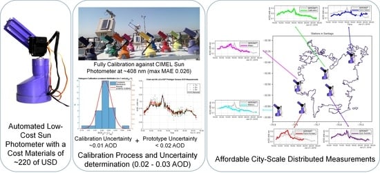
:We propose a monochromatic low-cost automatic sun photometer (LoCo-ASP) to perform distributed aerosol optical depth (AOD) measurements at the city scale. This kind of network could fill the gap between current automatic ground instruments—with good temporal resolution and accuracy, but few devices per city and satellite products—with global coverage, but lower temporal resolution and accuracy-. As a first approach, we consider a single equivalent wavelength around 408 nm. The cost of materials for the instrument is around 220 dollars. Moreover, we propose a calibration transfer for a pattern instrument, and estimate the uncertainties for several units and due to the internal differences and the calibration process. We achieve a max MAE of 0.026 for 38 sensors at 408 nm compared with AERONET Cimel; a mean standard deviation of 0.0062 among our entire sensor for measurement and a calibration uncertainty of 0.01. Finally, we perform city-scale measurements to show the dynamics of AOD. Our instrument can measure unsupervised, with an expected error for AOD between 0.02 and 0.03.
1. Introduction
Atmospheric aerosols are the small solid, liquid or mixed phase particles suspended in the air, with diameters ranging from 10 to 10m. These particles may be originated by natural processes (sea salt, volcano ashes or pollen), but also by anthropogenic sources (combustion engines, industries, wood burning) [1,2]. They also can accumulate and react among them in the atmosphere. Depending on their size, they can stay in the atmosphere for hours or days [3]. Aerosols impact on many areas, such as climate and health.
Aerosols have a complex effect on the earth’s energy budget. Depending on the aerosol properties, they may produce net cooling by reflection or scattering of the incident solar radiation, but also net heating when solar radiation absorption predominates [4,5,6,7]. Additionally, aerosols have a major impact on climate due to their role as condensation nuclei, necessary for cloud formation [8,9,10]. Moreover, the effects of aerosols are the largest sources of uncertainties in climate changes and weather predictions [11].
Besides the impact on the climate of aerosols, they can also produce important effects on human health. Exposure to airborne particulate matter and ozone has been associated with increases in mortality and hospital admissions due to respiratory and cardiovascular diseases [12].
The aforementioned context justifies the need for a better understanding of aerosol properties and their geographical distribution. However, modeling the generation and transport of aerosols is a challenging task [13,14]. Observational approaches based on satellites or ground-based instruments have shown promising results to support the models [15,16,17,18]. Although, these observational approaches still tend to present limitations in terms of costs, time availability or spatial extent and resolution.
Ground-based instruments such as particle counters, sun photometers and LIDARS measure in one place for a long time with a high cadence, having a good time sampling, but low spatial resolution due to the location constraints and costs of the instruments [19,20,21].
In contrast, aerosols can be measured from space. Low earth orbit satellites (for instance the MODIS radiometer) cover most of the surface of the earth but only passes twice per day at a given location [22], hence cadence is low. This issue has been addressed by geostationary satellites, such as GOES-16 or Himawuari-8. However, the spatial resolution for this type of satellite is poorer than that from lower orbit satellites. In addition, GOES-16 and Himawuari-8 have reported uncertainties for satellite products much higher than those from ground measurements [23,24,25,26,27]. In particular, for cities, the uncertainties of satellite products skyrocket due to the changes in the reflecto-properties of ground [28]. However, due to the cost of the current ground-based instruments, it is prohibited to use a high number of these instruments in urban areas, having available only limited distributed campaigns at regional scale [21]. Other examples of distributed campaigns involve hand-held sum photometers [16,29,30] to compare in situ measurements with satellite data for a short time (for example, some hours per day for a month) and cannot be maintained for a long time, due to the requirement of at least an operator per instrument.
In this article, we present a new low-cost automatic sun photometer (LoCo-ASP), together with its calibration method, capable of performing continuous and unsupervised measurements of aerosol optical depth. Its lower cost with respect to current market alternatives enables its use in an array, comprising several observation points in an urban-sized area. Hence, with this work, we start to solve the trade-off among cost, cadence and spatial coverage for the measurements of aerosols in cities.
LoCo-ASP was developed and tested in the city of Santiago de Chile (3327S 7040O), where the complex topography induces significant differences in the aerosol daily cycle, even for points located less than 15 km apart [16,17]. This variability was also part of the study motivation, since different aerosol concentrations could introduce inequalities in localized variables, such as solar energy production [31] or human health [32].
Section 2.1 presents an overview of our proposed solution, calibration method and operational strategy. Section 2.2 presents the measurement principle and hardware of the instrument. Section 2.3 presents the calibration strategy for several LoCo-ASP prototypes that would be later installed at different points in the city of Santiago. Section 3.1 compares a typical Langley calibration process with the proposed pattern-instrument method for several units. Section 3.2 studies the sources of uncertainty for the instruments and the calibration. Section 3.3 presents the testing of the calibration strategy with a real implementation of the aerosol monitoring network. Finally, in Section 4, the results are discussed, and Section 5 presents our conclusions, highlighting the main results and the lessons learned for future implementations of this urban aerosol monitoring concept.
2. Materials and Methods
The objective of this work is to continuously measure aerosol optical depth (AOD) with high temporal (every 5 min or less) and spatial resolution (10 km or less) at mesoscale (10–100 km).
Ground-based sun photometers are passive remote sensing instruments, capable of performing continuous AOD retrievals of the local atmospheric column. Therefore, a network of sun photometers should be able to provide as many observation points as available instruments. However, this approach is limited by the number of resources that are needed. Automatic sun photometers are expensive, and at present, it constrains the number of observation points in this scale. This partially explains why, in the AERONET or SKYNET networks, it is rare to find cities with more than one or two observation points [20,33]. Another approach is the use of handheld low-cost sun photometers. This reduces the cost of the instruments, at least an order of magnitude, yet limitations still appear by the need of individual operators at each measurement site (labor costs and/or limited time availability) [16,34,35].
Considering these restrictions, we develop a solution that combines the advantages of both automatic and manual instruments. To achieve our solution, we address the following goals:
- To design and develop an automatic sun photometer under a low-cost constraint.
- To calibrate and compare the instruments using a ground truth instrument (Cimel Sun Photometer [36]).
- To perform measurements at an urban scale. The calibration of the instrument shall assure that all the measurements from each instrument are comparable among them, with an acceptable level of uncertainty.
Step 1 is discussed in Section 2.2, step 2 in Section 2.3, and step 3 in Section 3.1, Section 3.2, Section 3.3.
2.1. Measurement Principle
Sun photometers use approximately monochromatic optical sensors to measure the spectral irradiance of direct solar radiation at specific wavelengths. When observing irradiance from the surface, its value will change depending on the solar constant, the solar angle, and an attenuation term introduced by the presence of gases and aerosols in the atmospheric column. This relationship is quantified by the Beer–Lambert law, presented in Equation (1) [37].
In Equation (1), represents the approximately monochromatic wavelength of the irradiance measurement. The term is the measured irradiance at the observation point, while is the irradiance at the top of the atmosphere. is the distance between Earth and the Sun at the moment of the measurement in AU. is the Rayleigh scattering optical depth and represents the extinction caused by Rayleigh scattering of solar radiation on air particles. represents the extinction of radiation due to absorption in the spectral bands of some atmospheric gases (especially oxygen and ozone). is the aerosol optical depth and corresponds to the integrated extinction of solar radiation by the presence of aerosols in the atmospheric column. This variable considers, at the same time, extinction due to scattering and absorption. Finally, m represents the relative airmass, with respect to the atmospheric column. Its value is a function of the zenith solar angle z, ranging from when (sun is at zenith), to when (sun is at the horizon). For z values under ⪅, m can be approximated by [38]. The operation of our prototype includes the use of larger angles. However, it requires the inclusion of atmospheric diffraction and Earth’s curvature effects [35,39].
Then, the aerosol optical depth for a wavelength can be retrieved by measuring the ratio between and , as indicates Equation (2).
Using the observation wavelength of the sun-photometer sensors, it is possible to calculate and ( is only necessary when is within a gas absorption band) [16,35]. m and are calculated from the sun position, associated with the coordinates and time of each observation [35]. Finally, the ratio can be estimated using the sun photometer sensor measurements. When exposed to sunlight, each sensor outputs a voltage directly proportional to solar irradiance ( in this context is the equivalent monochromatic wavelength of the photodiode [16,35]). Therefore, the ratio is equivalent to the ratio , where is a calibration constant associated with the sensor. This calibration constant can be retrieved using different methods, such as the Langley plot, or the intercomparison with reference instruments (see Section 2.3).
Hence, when the sensor calibration constant is known, can be estimated by combining the measured photodiode voltage with the theoretical calculation of the remaining terms.
2.2. Instrument Description
The instrument requires to detect the solar irradiation at a visible wavelength. To achieve this, the device is developed using LEDs working as photo-diodes. Those LEDs generate a small current when the sunlight is received. This current is proportional to the solar irradiance at the equivalent wavelength of the photo-diode. The current is amplified and converted to voltage through an operational amplifier. Finally, the voltage is digitized using an analog to digital converter (ADC) to be saved in a SD card. Those values can be used directly in Equation (2), as explained in Section 2.1.
In addition to the raw voltage, other parameters should be measured to calculate . In particular, we need to estimate the air mass m, the Rayleigh scattering , and the gasses optical depth .
The air mass m is calculated using the procedure presented by [39]. To calculate m, it is needed to know the zenithal angle to the sun. This magnitude can be calculated if the time of the measurement and the position of the instrument is known at the moment of the measurement. This information is gathered by using a GPS receiver, which was included in the instrument. The zenithal angle and are calculated using the algorithm introduced by [40].
The Rayleigh scattering is estimated using the approximation proposed by [41], which is dependent on the equivalent wavelength of the sun-photometer sensor. Moreover, depends on the amount of air over the instrument. This dependence is added using the ratio between the measurement’s place pressure and the sea level pressure. Therefore, a pressure sensor was included in the instrument.
In the case of the gasses optical depth , it depends on the wavelength of the measurement. The most important gasses to take into consideration in the visible spectrum are mainly ozone and water vapor. Both can be neglected for measurements near 400 nm, as demonstrated by [16].
LED sensors have a wide spectral response. Therefore, the equivalent wavelength () must be estimated [35]. In addition, the simulations performed by [16] demonstrated that, when the gasses effects are not present, a monochromatic sensor and a wide spectral sensor produce similar responses.
Furthermore, the Langley constant and the equivalent wavelength () are the calibration constants required to obtain a measurement. Typically, those constants are obtained using the Langley plot method and the spectral response of the photo-diode, respectively. However, this approach shows some issues, such as the place to perform a Langley plot calibration and the equipment required to study the response of the LED sensor. Those issues are magnified if we consider the calibration of several units of the same instrument. In Section 2.3, an alternative approach is proposed.
Here, is the equivalent wavelength of the LED-sensor; is the Langley constant; both must be obtained through a calibration process; is the airmass and z is the zenith angle at the time of the measurement. Moreover, is the measured voltage in the LED-sensor; P is the site pressure at the time of the measurement (both are measured), and is the atmospheric pressure at sea level (we use the typical value 1013.25 hPa).
In addition to the scientific requirements, the instrument should be automatic to allow measurements from different places at the same time, without human supervision and/or intervention. It must be low cost and simple to be manufactured in large numbers. In the following, we present the instrument architecture and how this device addresses the presented requirements.
Instrument Architecture
The instrument is an automated and upgraded version of the handheld sun photometer proposed by [16]. The improvements to the handhld version include a GPS to storage time and position, the capability to use four sensors instead of two, a more precise and faster analog to digital converter (ADC), and an upgraded amplification system. Moreover, it can work with a 12 V power source and a rain detector can be added (although not yet included in this version). All the custom components designs (parts and PCBs) are available in the project repository.
Regarding the sensor, we use the same kind of sensors for the four spaces in each prototype for simplicity in the calibration process and redundancy. This sensor is the same type of sensor used by [16]. It is a commercial 8000 mcd blue LED. The luminous intensity allows us to neglect the dark current of the sensor and the temperature effect in the semiconductor for a normal temperature range (between 0 and 40). Unfortunately, the vendor does not provide the model of the LED, but there is a previous characterization of the sensor response, with an equivalent wavelength around 408 nm [16].
Furthermore, the contribution to the optical depth due to absorptive gasses, such as ozone and water vapor, can be neglected according to simulations from [16]. In addition, the same article demonstrated by simulation that there is not a significant difference between using a sensor with a wide spectral response (for instance, a LED) or a monochromatic sensor if there are no external effects in the AOD. Therefore, we do not need an optical filter and only use a cover, thus we use direct light over the sensor.
The LoCo-ASP sun photometer can be divided into two main subsystems: the measurement subsystem and the robotic arm to track the Sun. The design philosophy was to improve technically the measurement system and emulate the human operation by the robotic arm.
While the measurement subsystem is in charge of gathering the measurements from different sensors, the robotic arm is in charge of turning on and off the instrument and aligning the sensors with the sun to perform measurements. To achieve the low-cost constraint, the proposed sun photometer uses low-cost commercial off the shelf (COTS) components. Since the LED is small, the arm resulted in a low-weight structure, which allowed the use of a low-cost motor to move the arm. The motor is a standard position servomotor (Model DSS-M15S with 270 degrees of range of movement).
Due to the low precision of the servo motors to point to the sun, the robotic arm is randomly moved around the estimated line of sight between the instrument and the sun. To guarantee measurements passing through the sun position, we use a high acquisition rate for measuring during the gathering period. The used analog to digital converter (12 bit MCP3204 ADC) can take 100 kilo samples per second (ksps). Considering the four sensors, each one of them is sampled 25,000 times per second. Moreover, the datasheet reports a speed of the servo motors of 3 milliseconds per degree. Therefore, the instrument samples 75 times per degree. That implies a resolution of 0.013 degrees per sample. Because the alignment and measurement processes are performed by different microcontrollers, there is no delay between sampling and tracking.
The development philosophy of the instrument consists of defining and designing different subsystems for the instrument, then testing each one individually. After that, a first prototype is assembled to develop the software and to improve the first designed hardware (doing changes in deficient subsystems) until a stable prototype was achieved. That approach allowed us to satisfy the scientific and operational requirements while maintaining the low cost of the instrument, with a final cost in materials close to 220 US dollars per prototype. The details of the bill of materials and their costs are included in Table A1 in Appendix A.1.
Figure 1 shows the main systems and components of the instrument, while the working procedure for each measurement is described as follows:
- The alarm clock indicates the Sun tracker CPU when starting a measurement.
- The sun tracker CPU gets time from the alarm clock and sets the alarm for the measurement.
- The sun tracker CPU calculates the sun position and defines whether the sun position is too low to measure AOD (night time).
- If the internal calculation of the sun tracker CPU defines it as good to measure, the CPU turns on the servomotors and sets them to the calculated sun position.
- Due to the low precision of this estimation, the sun tracker also uses the solar sensor to improve the sun position estimation, and moves the servos around the estimated alignment position.
- The sun tracker CPU turns on the photometer CPU to start measuring. At the same time, the Sun tracker continues moving the servos around the alignment position.
- The photometer CPU takes measurements of for one and a half minutes. It only saves the highest measured values.
- After one and a half minutes, the sun tracker moves the servos to the park position and turns them off.
- The Photometer CPU gets the time and position from the GPS module, the pressure and temperature from the barometer and temperature sensors, and from the LED, saving all of them in the SD card.
- The sun tracker CPU turns off the photometer CPU and waits until the next measurement time.
The measurements where a cloud is present must be removed. To do that, we implement an outlier remover. We calculate each measurement slope with its neighbors in the time series (the measurements immediately before and after) and calculate the difference between both slopes. For a single day, we calculate the quartiles of the calculated quantities and remove all measurements over the third quartile, plus 1.5 the difference between the first and the third quartile, and under the first quartile and the same difference. This method is useful to remove single outliers. However, for longer times with clouds, defective measurements must be removed by hand.
2.3. Instrumental Network Calibration
The calibration procedure of a LED-based sun photometer consists of determining and . To obtain , we need to know the sensor response spectrum and to estimate the center of the spectrum [35]. In addition, [16] showed through simulation that there is not a significant difference between the estimation and a monochromatic sensor response for the case of LED-based sensors in wavelengths when is negligible.
To obtain , the Langley plot extrapolation method [16] is usually used. This method consists of taking several measurements at different sun altitudes with a stable level of aerosols. By using Equation (1), it is possible to obtain Equation (4). If we consider that does not change in all the measurements, we will have a linear equation where the airmass m is the independent variable and the dependent variable. Both variables can be obtained using the instrument and knowing the place and the time of each measurement. Therefore, it is possible to estimate using a linear regression.
However, the conditions required to perform a Langley plot calibration are difficult to achieve. Calibration sites are usually in high-altitude places without important sources of aerosols nearby [42]. This issue is more difficult to address if we consider the number of instruments that need to be calibrated in the case of sun photometer networks. For instance, the AERONET network only calibrates using this method for two of their instruments, which are used as pattern instruments to calibrate the rest of the network [20].
We propose a calibration process using an AERONET Cimel Sun Photometer as a pattern instrument to calibrate our prototypes. The challenge of our case compared with the calibration of AERONET instruments is the fact that the equivalent wavelengths are different between the Cimel sun photometer and our instrument. Fortunately, there is a method to interpolate from two other aerosol optical depths at different wavelengths.
Equation (5) shows the Ångström exponent equation [43]. This equation allows us to determine any aerosol optical depth by knowing and an aerosol optical depth at any wavelength. The exponent is called the Ångström exponent, and can be estimated by using Equation (6). This exponent is also related to the particle size distribution of aerosols [44]. In practice, we only use Equation (6) to calculate the aerosol optical depth given two wavelengths, the optical depth for one of them and the Ångström exponent.
Using Equation (6), we can estimate the AOD from the original Cimel measurement bands ( and in Equation (6)) to the equivalent wavelength of our instruments. We only have to change one of the wavelengths for the desired new wavelength, as shown in Equation (7), where is the wavelength, where the AOD wants to be estimated.
We propose to calibrate our prototype instruments by taking measurements next to the pattern instrument and then adjusting and using non-linear least-squares optimization. Equation (8) exhibits the cost function. All the functions where is a variable are decreasing, while is an increasing function. The optimization equation is a square difference between a decreasing and an increasing function. Therefore, the cost function always has a minimum in the cases where can be neglected.
In the case of our prototype, we used the same blue LED studied by [16] for all the measurements, which has a sensor response spectrum between 350 and 450 nm (a typical sensor response can be seen in Figure 2) with an equivalent wavelength near 408 nm. In the same article, it was demonstrated that the absorption spectrum by atmospheric gases can be neglected at regions with no absorption (for example, O and water vapor).
Moreover, there are other trace gases such as SO and NO near the response band of the sensor. In the case of SO, their absorption bands are under 350 nm [45], which means, the SO is outside the sensor response band. In the case of NO, it is absorption fall in the LED-sensor response band [46]. However, the reported estimated error for high concentrations of NO events is around from MODIS satellite AOD estimations [47]. In our case, we measure AOD values under 0.45, which means an expected error due to NO lower than 0.005, which is under the expected AOD error for our sensors (higher than 0.01). In addition, we consulted the NO concentration using TROPOMI NO data [48] for the calibration and measurement days. From this search, we can tell that there were no relevant events that could affect the measurements. Thus, we neglect the NO effect in our estimations and measurements. However, this NO checking procedure will be included systematically to future campaigns.
For that reason, we can use the optimization process proposed before without any additional consideration. The main advantages of this process are that it is not necessarily a calibration site with constant aerosol optical depth and to know the sensor response (if there is no significant gases effect in the response band of the sensor). Furthermore, the measurements are immediately comparable with the pattern instrument, and can be re-calibrated if the pattern instrument is calibrated after the measurements. On the other side, an important disadvantage is that all the systematic errors are transferred from the pattern instrument to the prototype. Another important disadvantage is that we are estimating the wavelength, so it will have some uncertainty associated.
3. Results
First, we need to check if the proposed calibration method is comparable with typical calibration methods. Section 3.1 compares the results from a Langley plot calibration and our proposed calibration process. Then, we determine the uncertainties of our prototypes, comparing the measurements after calibration of different sensors and studying statistics in the determination of the calibration constants. These results are presented in Section 3.2. Finally, we exhibit some field campaign results in Section 3.3 to demonstrate the utility of this kind of instrument in urban aerosol studies.
3.1. Comparison between Langley Plot Calibration and Optimization Process
As a first approach, we perform a Langley plot calibration and compare the calibration constants with the proposed calibration process. The chosen place for the Langley calibration was Valle Nevado at the East of Santiago de Chile and around 3000 m.a.s.l. This place has a low and stable optical depth. However, it is near a city and the aerosols could anyway affect the optical depth there. In the case of the optimization process, we use the Cimel sun photometer of the Santiago Beauchef station. Those kinds of instruments are part of the AERONET sun photometer, and they are considered as ground truth [21].
Figure 3 shows the results of the Langley plot calibration process, while Table 1 and Table 2 exhibit the differences in the calibration constants obtained by both calibration processes. The results show a mean difference around 1% and a variation around 1% among all the sensors used for the experiment. In the case of the Rayleigh constant, we compare the results with the mean value used by [16] for the same sensor: 408 nm and a Rayleigh constant of 0.033.
Regarding the Langley constant, the mean difference between both calibration methods was −0.09 (−1.10%) for all sensors, while the standard deviation was ±0.13 (± 1.61%). In the case of the Rayleigh constant, there is not an average difference between the estimations, but the standard deviation was ±0.03 (± 7.84%). This means that the calibration constants are similar from both methods, although there is a bias in the Langley constant estimation.
This experiment has some limitations. On one hand, the Langley plot calibration was performed in a place near the city, thus the conditions to perform the calibration were not optimal. On the other hand, we only compare two single-day calibrations using both methods. However, the differences between the calibration constants and the Langley plot from Figure 3 are close enough to verify the proposed calibration method to retrieve reasonable Langley constants as a first approach.
In essence, our prototype can perform a Langley plot calibration, and our proposed calibration method can retrieve the calibration constants with an undetermined uncertainty.
After calibration, it is useful to know the difference between the measurements of our prototypes and the pattern instrument. Figure 4 shows a scatter plot with measurements of one sensor after calibration and the Cimel sun photometer. The details for each sensor are in Table A2 in Appendix A.2. These results show that after the calibration process, the mean difference among the measurements of the Cimel sun photometer and our sensors (4 in an instrument) can be neglected (the mean bias for all the measurements is 0.0002), while the variation is represented as the maximum root mean square error (RMSE) is 0.068, and the maximum mean absolute error (MAE) is 0.026.
At the beginning of the AERONET program, the reported error for the Cimel instruments was 0.02 if the wavelength was under 550 nm [20]. Nowadays, the reported error has decreased to 0.01 [21]. Furthermore, there is an increase in the error estimation when we calculate the AOD in our equivalent wavelength from original AERONET sun photometers wavelengths using Equation (7). We found by propagation that the error of from the AERONET sun photometer is around 0.0131, in the mean case of Santiago (a detailed explanation is included in Appendix A.2). As a result, the variation of our instrument is comparable with those errors.
Similarly, in Figure 4, the linear regression presents a slope of 0.98, which is an error around 2% between both instruments. Otherwise, if we consider the estimation error from the AERONET Cimel sun photometer of 0.0131 and the max of AOD measurement range (around 0.45 from Figure 4), the uncertainty is around 2.9% (for lower values, this value increases). Thus, this difference is under the significance level of the measurements, and can be neglected.
3.2. Uncertainty Estimation
The uncertainties in the measurement can come from two main sources: the calibration and the internal prototype differences. For that reason, we perform experiments to identify both error sources. First, we measured and calibrated several prototypes at the same time, and compared the same measurements after calibration. Then, we performed calibration for a single prototype for several days to identify the variability in the calibration process.
3.2.1. Prototypes Uncertainty
To perform a city-scale campaign, we need to manufacture and calibrate several prototypes. However, measurements are subjected to uncertainties. For example, uncertainties are introduced by misalignment when aiming at the sun or sensor noise. For that reason, we compare the measurements of the sensors under the same conditions to determine the uncertainties in the AOD estimation among different prototypes.
We measure together with the Cimel sun photometer and seven of our LoCo-ASP prototypes over the course of two days (26 November and 27 November 2018). To avoid differences among the systematic calibration errors, all the prototypes were calibrated with the measurements of the first day. The measurements of the second day were used to compare among them. In other words, we calculated the mean and the standard deviation of our prototypes measurements for each measurement time (we have 28 measurements every time).
Figure 5 presents a comparison among different sensors’ measurements for the same place and time. In other words, all the calibrated prototypes are measuring at the same time and place. The top panel shows the standard deviation for the join measurements for all sensors each time, while the down panel shows the single measurements for each sensor. Red dots are the measurements under one standard deviation, green dots between one and two standard deviations, and blue dots over two standard deviations. The black line corresponds to the AERONET Cimel sun photometer equivalent AOD at 408 nm.
Those results show that the standard deviations for all the measurements at the same time are always under 0.02. Moreover, the sensors follow the measurements of the pattern instrument after calibration (most of the red dots are around the black line). Finally, the mean bias for the measurements and the Cimel sun photometer was −0.0017, while the mean of the standard deviation from the top panel is 0.0062, as Table 3 shows. These results are comparable with the reported error for the Cimel sun photometer, under 0.02 for [20] or 0.01 using the newer estimation techniques [21].
3.2.2. Calibration Uncertainty
An important advantage of an automatic sun photometer is the number of days that it can measure without important surveillance, compared with a handheld sun photometer that requires a human operator. This feature allowed us to measure, together with the pattern instrument, one of our prototypes for 32 days during January and February of 2019 (summer break at the southern hemisphere).
Every day, we performed the calibration process and obtained the equivalent wavelength and the Langley constant. In other words, we obtained several estimations of the calibration constants to study the statistical distribution of our calibration process. This experiment was inspired by the work performed by [42] in the AERONET Cimel sun photometers.
Regarding the proposed calibration process, we used Equation (8) to estimate the Langley constant and the equivalent wavelength for the sensor. The uncertainties from both variables are coupled because of the optimization process. In other words, the real uncertainty for the calibration process must include the contribution from both variables at the same time and not each one independently, since these errors always have opposite signs.
To estimate the calibration error, we need to consider the two first elements that compound the calibration equation, Equation (9). In this equation, each calibration constant is separated (Langley constant first and equivalent wavelength second). It is possible to see that the Langley constant is divided by the air mass, while the Rayleigh scattering () is multiplied by the pressure ratio between the local pressure and the sea level pressure. Therefore, both magnitudes are involved in the calibration error estimation.
Figure 6 shows a histogram of with and . We performed the Kolmororov–Smirnov test with a of confidence level to check if the distribution can be considered as a normal distribution. The results indicate that it can be considered as a normal distribution at that significance level. In addition, Table 4 presents the mean and the standard deviation of the calibration constant. From this table, the accuracy in the estimation is ± 3 nm, while the errors of and are around ±0.01 and ±0.02.
The distribution of calibration constants does not exhibit degradation of the sensor for the time of the experiment, requiring longer measurements to determine a degradation rate. Figure A1 and Figure A2 in Appendix A.3 present the obtained calibration constants over time.
Finally, Figure 7 presents different standard deviations for different values of and . In general, the calibration error is under 0.01. Adding this magnitude to the error among the prototypes gives us an expected measurement error between 0.02 and 0.03.
The Langley constant error achieves the maximum contribution when the air mass is near the unit because in Equation (9), the air mass divides the Langley constant. While the air mass increases, the contribution of the Langley constant in AOD decreases. For high air mass values, we only have the contribution from the equivalent wavelength estimation error through in Equation (9). Because of the calibration procedure, the Langley constant error and the equivalent wavelength error always have opposite signs in the AOD estimation.
3.3. Network Measurement Case Studies: Santiago de Chile
3.3.1. Case Study: 30 July 2018
The objective of the first experiment is to verify whether we can repeat previous results obtained using manual instruments with our new automatic sun photometers. Indeed, previous AOD measurements made by [16] relied on a similar instrument, but it is a manual one. This manual instruments were able to reproduce Cimel measurements and provide some observations of the AOD life cycle in a city, Santiago. Specifically, these observations validated previous results from models, that predicted the increase of aerosol concentration at downtown in the morning, due to an increase of local emissions, which are later transported eastward by the valley circulation in the afternoon [49].
Figure 8 presents the results of the campaign of the 30 July 2018, where we observed the aforementioned behavior, but this time using our new automatic sun photometers (LoCo-ASP). The instruments were installed in a similar disposition, time of the year and atmospheric conditions with respect to the [16] study. They are placed ∼13 km apart from each other, at the city center (downtown, Santiago Beauchef site), east (La Reina) and south (La Florida). AOD is measured the full day, using a Cimel sun photometer at the Santiago Beauchef site, and two LoCo-ASP sun photometers at La Reina and La Florida sites. The calibrations of the LoCo-ASP sun photometers were done following the procedure described in Section 2.3. The beginning and ending times of the samples are only limited by the hours with direct solar radiation at each site, which may be influenced by the local topography.
Results are consistent with previous observations and models. Indeed, the upper panel shows that AOD starts to increase first at downtown, by 10:00 local time (14:00 UTC). High values of AOD last for about three hours, after which it has a sharp decrease by 18:30. This decrease at downtown coincides with a simultaneous increase in AOD at the eastern side of the city (La Reina), which had a much lower AOD value until that time. This behavior is compatible with aerosol displacement eastward, and matches the results previously modeled and observed [16,49]. Later in the day, by 19:45, there is a new sharp increase in AOD at the Santiago Beauchef site. This is explained by aerosol re-circulation above the boundary layer, happening during the evenings due to orographic airlifting on the slopes of the Andes mountains [50].
Meanwhile, the lower panel shows that the behavior at the south of Santiago follows a cycle that is closer to what is observed in downtown, with a delay of AOD peaks of approximately one hour and slightly lower AOD values. This may indicate that some aerosols move from downtown to the south, since local aerosol production in the southern part of the city is lower (it is mainly a residential area). The study of this and other hypotheses would benefit from the installation of more observation points (to reach the desired spatial resolution of 5 km or less), which is the motivation of the case study of Section 3.3.3.
3.3.2. 12 December 2018
The case presented in Figure 9 shows the significant spatial variation of aerosols in small areas. In this campaign, we used three LoCo-ASPs: the first was placed next to the AERONET station in Santiago Beauchef, in the border of downtown (Calibration unit, upper panel), the second was in Juan Gomez Milla Campus of the University of Chile in the east of the city (Ciencias, middle panel) at 6.5 km from the first one, and the third was in Cerro Calan in the northeast of the city (Cerro Calan, lower panel) at 9.6 km from the second station and 13.7 from the first one.
The data exhibit an increase in AOD around midday, and the displacement of this increase to the east and the northeast during the afternoon. Another relevant observation is an increment of AOD during the morning in Ciencias station. Furthermore, there is another increase during the afternoon for all the stations. On one hand, the higher increase displacement follows the typical behavior observed by [16] and modeled by [49]. On the other hand, the minor displacements may be explained by the human activity of the city.
Inside the triangle of the measurement points, we can find Santiago’s downtown and the commercial and financial centers of the city. Most of the population lives south of this area (in the southeast of the city). During the morning, the displacements of people are from outside to inside the triangle. Meanwhile, in the afternoon, the displacement is in the opposite direction. The increase in AOD in Ciencias station in the morning may be related to the displacement of people from the south. However, more points are needed to understand where the aerosol sources are now, and how they move into the city daily.
Moreover, [31] presented the annual mean AOD using measurements from the AQUA satellite product. This satellite usually measures the area of Santiago during the afternoon and the results of the article exhibit that there is an aerosol concentration in the area covered by our LoCo-ASP stations. Thus, the measurements presented in this campaign support this evidence, although the general behavior of AOD is more complex during the rest of the day.
3.3.3. 21 January 2019
In this case, we placed six units of LoCo-ASP from the southwest to the northeast. According to the models, this is the mean wind direction in Santiago city [49]. Two of these instruments were placed outside the city in the southwest (Malloco and Padre Hurtado stations). One LoCo-ASP was placed on the border of the city (Maipu station), and two near the center (AERONET, which is the control instrument next to Santiago Beauchef AERONET station, and Gran Avenida). The last instrument was placed in Cerro Calan station. Unfortunately, Ciencias prototype was not available that day.
Figure 10 shows a map with the prototypes position of each instrument in the city. The other panels present the time series for each station on that day. The AERONET station is presented in the upper panel and the other stations from the west to the east, from upper to lower panels. Some points were removed due to obstacles in the measurement site such as trees or towers.
From the data, the Malloco station does not show any important AOD increment during the day. However, all other stations present a rise displaced in time and moving from the southwest to the northeast. This behavior is similar to that presented in Figure 9; the main difference is that the increment of AOD started between Malloco and Padre Hurtado stations, and then moved towards the city. This result clearly exhibits the utility of Sun Photometer Networks at a city scale, which allowed us to capture the rich dynamics of aerosols in Santiago.
4. Discussion
In this work, we present three main contributions. First, we developed a monochromatic low-cost automatic sun photometer (LoCo-ASP) for AOD measurements. Second, we proposed and evaluated a calibration algorithm. The algorithm uses a pattern instrument to calibrate the LED-based sensors to estimate the unknown Langley constant and equivalent wavelength. The method takes advantage of the gasses contribution to the optical depth, and can be considered negligible at the operation wavelength; this is the reason for the chosen LED used in the LoCo-ASP. Finally, we performed city-scale measurements with several units to evaluate the performance of the instruments by comparing the AOD behavior over Santiago with previous works that used simulations, satellite data and handheld sun photometers.
4.1. LoCo-ASP Instrument
Regarding the photometer, we achieved an instrument with a cost of material near 220 dollars. This cost is comparable with the cost of LED-based handheld sun photometers. For instance, the reported cost of materials for the photometer presented by [16] is around 150 dollars. The low cost per unit of this work was achieved by avoiding oversizing the components and subsystems. In addition, the replacement of the user interface components (e.g., display) by the automatic subsystem also helped to reduce the cost.
The quality of the measurements has been estimated and compared with the pattern instrument. We obtained a maximum RMSE of 0.068 and a maximum MAE of 0.026. The maximum MAE is comparable with the reported error for the AERONET network at its beginnings (0.02 for wavelengths under 550 nm [20]). Nowadays, after improvements in the AERONET procedure, the reported error has improved to 0.01.
In the case of the MAE, the maximum value was 0.026, with only three of the 38 sensors tested over 0.02 (92% of the sensors had an MAE under 0.02). Similarly, the maximum value of the RMSE was 0.068, but only four of the 38 sensors had an RMSE over 0.03 (89% of the sensors had an RMSE under 0.03). The difference between the MAE and the RMSE indicates measurements with large error in some sensors, this can be due to the fact that we use a less conservative procedure, compared with the Cimel sun photometer [20], to estimate and remove measurements affected by clouds or misalignment.
The work developed by [16] reports an RMSE of 0.009 for the same LED sensor used in this work. However, these results were limited to three sensors with less than 200 measurements per sensor. These instruments required knowing the spectral responses of the sensors and be calibrated by a Langley plot procedure performed in a proper location. In our case, we performed measurements for 38 sensors, without the necessity of knowing the LED’s spectral responses and a Langley plot calibration. This number of sensors were distributed in ten prototypes of sun photometers with average measurements per sensor of 1340. This number is higher than the typical number of calibration measurements for handheld photometers, such as [16] or [51], mainly due to the automation of the instruments.
Furthermore, we could compare our measurements among our prototypes after calibration. Figure 5 shows that the standard deviations for all the AOD measurements were under 0.02, with a mean standard deviation of 0.0062 for all the measurements. This result gave us an independent error estimation comparable with that obtained by the MAE (under 0.026, with a 90% of the sensors under 0.02) and RMSE (under 0.068, with a 89% of the sensors under 0.03), which compares the difference between a prototype and the pattern instrument.
The main limitation of our instrument is the number of wavelengths available. To enhance their capabilities, we need to include more wavelengths to estimate the Ångström exponent, which relates to the particle size distribution. Other possible improvements are to increase the reliability of the instrument and develop the subsystem to remotely access the instruments and their data.
4.2. Calibration Procedure
The proposed calibration procedure provides several advantages. We only need a pattern instrument to calibrate the low cost instruments, instead of the facilities to characterize the spectral response of the sensor and the place to perform a Langley plot calibration. Typically, for handheld sun photometers, it is only possible to perform a calibration over the course of one or two days [16], since it requires a person that needs to be exposed to the sun radiation, which in the end is a risk to his/her health. We compared a Langley plot calibration with our calibration method, the results differ around −1.1% in average and 1.61% in standard deviation. Taking into consideration that the calibration place was not the most suitable (high but close to the city) and the limited availability number of Langley calibrations, the results are comparable.
In the case of the automatic sun photometers, we could stay measuring next to the pattern instrument for 32 days with one prototype (the others were usually distributed around the city for measurements). With this amount of data, we could obtain a more reliable statistic for our calibration, being able to verify the distribution of our calibration constants and estimating the error with higher precision. Similar work was developed by [42] to study the calibration sites for the AERONET sun photometers. The current work has provided the data to replicate those analyses with our prototypes. Moreover, the procedure allows the simultaneous calibration of several units without moving them to a high isolated site, facilitating the implementation and operation of a sun photometer network. Figure 6 exhibits a Gaussian behavior in the calibration error, this result shows the actual performance of the instrument, and it can be used to improve the calibration process.
Regarding the degradation of the sensors, the data collected are not enough to determine a degradation trend. For instance, Ref. [42] reports a degradation of 0.4% in 5.6 years of calibrations for the Cimel sun photometers. In our case, we only have continuous calibration constants for 32 days. Therefore, we need to measure for a much longer time to study the sensor degradation. Thus far, we can guarantee that the degradation of the calibration is negligible in a month-long period. We can adapt the operations to this period. For instance, if we cover a city of 25 km by 25 km with 25 instruments, the spatial resolution might be close to 5 km. If we have some extra well calibrated instruments, we might take each instrument for recalibration every 25 days, leaving a spare instrument at the location where the removed-for-calibration sun photometer was measuring. The frequent re-calibrations will allow the study of changes in calibration constants. This approach permits us a degradation study in the long term, without affecting the quality of the measurements.
The main advantage of this calibration process is that AOD measurements are directly comparable with the measurements of the pattern instrument. If the pattern instrument is part of a larger network, the data can be confidently added to the network data base. Moreover, past LoCo-ASP measurements can be corrected with new calibration constants in the pattern instrument if this is re-calibrated.
However, this process has some disadvantages. One of them is that this process transfers all systematic errors from the pattern instrument to our device. In addition, the current calibration procedure requires that the gasses optical depth () is negligible at the wavelength band of the used LED-sensor. This is true for the currently chosen LED, but must be taken into consideration if the number of wavelengths (LEDs) is extended. This can be useful to estimate the Ångström exponent.
4.3. Case Studies
The case studies have demonstrated the capabilities of a sun photometer network at a city scale. We showed, in our case studies, the different behavior of AOD at different points inside the city of Santiago (Chile), which justify the increment of measurement points. We were able to find sources and variations of AOD. Satellites, which have a higher spatial resolution, cannot measure with this level of precision AOD, due to the uncertain reflecto properties of the ground. In addition, low orbit satellites cannot capture the aerosol dynamics, due to poor temporal resolution. Figure 8 presents a good motivation to implement more than a unit per city, while Figure 9 and Figure 10 show displacements of AOD during the day from the southwest to the northeast, and local emissions of aerosols. Furthermore, the results are coherent with simulations [49] and satellite measurements of AOD in Santiago [31].
We have presented results coming from some preliminary campaigns. However, the city-scale campaign concept has some challenges that can be considered. One of them is to find optimal places to install the instruments. For instance, the calibration process is performed in a terrace specially adapted to facilitate long term measurements, while during the campaigns, the instruments are placed, in many cases, on sub-optimal places to avoid shadows during the day, such as the rooves of houses, with a simple installation and verification protocol (usually using electrical extension to provide energy). These differences in measurement conditions can impact on the quality and fidelity of the gathered data. The operational conditions can also impact on the capacity of instruments to stay properly measuring. For instance, an unfavorable installation can facilitate rollovers with wind and earthquakes (something frequent in Chile). Sub-optimal places are difficult and prolong the installation and removal processes. Thus, the reliability of the network can be improved by adapting places around the city to facilitate the installation of the instruments, and providing connectivity, either to verify the state of the instrument or to communicate the data (facilitating the logistics). These changes can have an increase in the cost of the system. However, it can vary from one city to another.
The case studies have shown the potentialities of a sun photometer network. A glance at these potentialities was presented by [16]. However, in this work, we have filled the gap for an automatic sun photometer network, based on a low cost instrument to improve the reliability of measurements in metropolitan’s areas. We identified the requirements to develop a sun photometer network, and implemented a small automatic network based on these requirements.
A sun photometer network can help us to better understand the behavior of aerosols inside cities during the day. This information can improve the understanding of the local weather and the development of public policies to mitigate the pollution. Future work can include performing larger campaigns (with more units by longer times), combining our measurements with data obtained by other means (such as models and satellite products), and extending the wavelength channels to provide estimations of the particle size distribution.
To estimate the particle size distribution, there are several challenges. We need to increase the number of wavelength channels to calculate the Ångström exponent with good accuracy. This implies improving the calibration method by including the gasses effect on the AOD estimation.
5. Conclusions
In this work, we achieved the development of an automatic low-cost instrument capable of taking measurements automatically, with similar accuracy compared with other ground sun photometers. We also proposed a calibration procedure, which was compared to the typical Langley plot calibration. In addition, we estimated the uncertainties of the measurements due to constructive variation among prototypes and the calibration process. Finally, we presented some cases of study to show the capabilities of an automatic sun photometer network.
The LoCo-ASP instrument, introduced in this work, has an estimated cost of materials around 220 dollars per prototype. The comparison between the Langley plot calibration and our method gave an error of −1.1% on average, and a variability of 1.6%. The results of the uncertainty estimation exhibit a mean standard deviation of 0.0062 for all the sensors measuring at the same time, and an error of 0.01 due to calibration uncertainties.
Additionally, we performed a field campaign with 7 LoCo-ASP in several places in the city of Santiago (Chile). The results of those tests show a rich dynamic aerosol behavior in the city with generation and transportation of them through the city along the day. The results are in line with wind simulations and satellite AOD measurements. The LoCo-ASP accuracy is comparable to commercial (mid-cost) sun photometers, although it has to be improved to achieve the accuracy of the best commercial sun photometers (e.g., Cimel). However, the LoCo-ASP accuracy is better than that reached by AOD measurements gathered by low orbit and geostationary satellites. Thanks to the low cost of the LoCo-ASP, the number of possible points might allow a spatial resolution in cities of 5 km or better at a high cadence.
With this work, we identified the gap that we wanted to cover with this instrument and the requirements to develop it. Going over cities is complex to measure aerosols. There are too many random sources of aerosol with complex and changing topographies (buildings, structures, parks, etc.). To capture this, dynamic behavior requires many measuring points (25 to 100) to gather data at a high cadence (at least one sample every 5 min). The measurement can be performed either from ground or space. The measurements gathered from the ground tend to be more accurate than those taken from space, mainly due to the uncertainties of reflecto-properties of ground in cities. Although the automatic ground instruments are less expensive than satellites, they are still prohibitively expensive to be deployed in large numbers in cities, especially considering the numbers of cities that might require monitoring. The commercial automatic ground instruments are currently used for gathering data at a regional level (resolution of 100 km). There are also commercial handheld sun photometers, which are less expensive than the commercial automatic instruments. However, the handheld instruments require operators, which makes mid- or long-term campaigns practical. The proposed instrument in this work, the LoCo-ASP, is at least two orders of magnitude cheaper than automatic ground-based instruments. This cost will allow us to have the required number of measuring points, with a similar cost to having an additional commercial automatic instrument (e.g., Cimel). It can perform campaigns at least an order of magnitude longer (from few days to few months) at high cadence, since it is automatic. However, a technician is required to perform logistic, maintenance and programmed calibration of the instruments. The accuracy of the instrument is much better than satellite products, similar to the commercial handheld sun photometers, and only half of automatic ones. Future work should be oriented toward increasing the reliability of the instrument for field campaigns and estimation of the particle size distribution of aerosols by increasing the number of channels available.
The geographic and atmospheric conditions for Santiago de Chile are well known compared with other cities. It would be of interest to test this in less studied cities, where aerosol dynamics are still not understood. Therefore, we need to expand the studies to other places and add more stations to achieve a better spatial resolution.
In summary, our concept allows precise and automated measurements at a low cost per unit. A complete application of this kind of instrument would be useful for the characterization of aerosol dynamics in complex areas with several sources, diverse surfaces, and different geographic relief and wind profiles.
Author Contributions
Conceptualization, C.G. and M.D.; methodology, C.G., M.D. and R.R.; software, C.G.; validation, C.G., M.D. and F.T.; formal analysis, C.G.; investigation, C.G.; resources, M.D. and R.R.; data curation, C.G. and F.T.; writing—original draft preparation, C.G. and F.T.; writing—review and editing, C.G., F.T. and M.D.; visualization, C.G.; supervision, M.D.; project administration, C.G.; funding acquisition, M.D. and R.R. All authors have read and agreed to the published version of the manuscript.
Funding
This research was funded by the Air Force Office of Scientific Research under award number FA9550-18-1-0249, CONICYT-QUIMAL 190004 and CONICYT-PFCHA/MagísterNacional/2018-2218120.
Data Availability Statement
All data used in this work can be found in https://github.com/spel-uchile/Fotometro-V3, (last accessed on 21 October 2021), where there is information regarding the instrument design and the data collected and processed for this work.
Acknowledgments
The authors would like to acknowledge Marcos Díaz’s family for allowing La Reina, Maipu and Gran Avenida station measurements.Thanks to Jose Miguel Campillo and Patricio Mella from the Department of Geophysics at the University of Chile, who helped us to install some prototypes. Thanks to Nicolás Hunneus, his family, and Luis Merchant for allowing the Malloco station installation. In addition, we want to thank to the Juan Alejandro Valdivia from Science Faculty at the University of Chile for letting us install the Ciencias station, César Fuentes for helping us with Cerro Calan station, Cristobal Garrido’s Family for La Florida Station, to Humberto Luhr for the use of his house in Padre Hurtado, and to MCI company for helping in the initial design of the prototype. We acknowledge the free use of tropospheric NO column data from the TROPOMI sensor from www.temis.nl. and the AERONET network.
Conflicts of Interest
The authors declare no conflict of interest. The funders had no role in the design of the study; in the collection, analyses and interpretation of data; in the writing of the manuscript, or in the decision to publish the results.
Appendix A
Appendix A.1. Cost of Materials of the Instrument

Table A1.
Cost of Materials for the LoCo-ASP Sun Photometer.
| Component | Cost (US) | Units | Total Cost (US) |
|---|---|---|---|
| Arduino UNO | 22 | 1 | 22 |
| Arduino pro mini | 9.95 | 1 | 9.95 |
| PCB Sun Photometer Sensor | 5 | 0.2 | 1 |
| PCB Robotic Arm Shield | 5 | 0.2 | 1 |
| LEDs | 0.5 | 8 | 4 |
| Amplifier LMC6484 | 3.88 | 2 | 7.76 |
| ADC MCP3204 | 4.06 | 1 | 4.06 |
| Electronics Components | 10 | 1 | 10 |
| Pin Headers | 10 | 1 | 10 |
| Cables | 10 | 1 | 10 |
| Case | 10 | 1 | 10 |
| Logger Shield | 49.95 | 1 | 49.95 |
| Servo Motor 270 | 14.9 | 2 | 29.8 |
| SD Card | 9.95 | 1 | 9.95 |
| Power Supply | 12 | 1 | 12 |
| BMP180 | 9.95 | 1 | 9.95 |
| DS3231 RTC Clock | 17.5 | 1 | 17.5 |
| Total | 218.92 |
Appendix A.2. Difference Comparison between Cimel Sun Photometer and LoCo-ASP
In this section, we present the detailed algebra to estimate the uncertainties of obtained from Equation (7) and the complete table with the difference for each sensor measurement with the estimated .
From Equation (7), we need to estimate the error from and . For the first one, we assume the error reported by [21] of 0.01. For the second one, we assume that there is not an error in the wavelengths and the only uncertainty is due to . To estimate this error, we use the equation presented by [52], Equation (A1).
Here, is the uncertainty of the Ångström exponent, while and are uncertainties from the AOD measurements from the original wavelengths from the AERONET cimel Sun Photometer. In both cases, we assume an uncertainty of 0.01.
The uncertainty for is given by Equation (A2)
For simplicity, to propagate the error, we assume that there is no correlation between and . Thus, the estimated uncertainty is a lower bound of the real one. Equation (A3) shows the estimate error from Equation (7).
Finally, to estimate this value, we used the mean AOD for the year 2019 in Santiago Beauchef 2 station in the wavelengths of 380 nm () and 440 nm , and the Ångström exponent of . The result was an estimated uncertainty of 0.0131 for nm.
On the other side, Table A2 presents the average difference and standard deviation between Cimel and each sensor.
Table A2.
Average difference and standard deviation between Cimel and each sensor.
| Unit and Sensors | Number of Measures | Average Difference | RMSE | MAE |
|---|---|---|---|---|
| Unit 1, Sensor 1 | 4575 | −0.0003 | 0.016 | 0.011 |
| Unit 1, Sensor 2 | 4641 | −0.0009 | 0.021 | 0.013 |
| Unit 1, Sensor 3 | 4093 | −0.0004 | 0.036 | 0.024 |
| Unit 1, Sensor 4 | 3362 | 0.0040 | 0.043 | 0.016 |
| Unit 2, Sensor 1 | 1532 | −0.0011 | 0.019 | 0.010 |
| Unit 2, Sensor 2 | 1336 | −0.0034 | 0.013 | 0.011 |
| Unit 2, Sensor 3 | 1561 | −0.0009 | 0.016 | 0.010 |
| Unit 2, Sensor 4 | 1195 | −0.0007 | 0.023 | 0.011 |
| Unit 3, Sensor 1 | - | - | - | - |
| Unit 3, Sensor 2 | 1371 | 0.0001 | 0.013 | 0.010 |
| Unit 3, Sensor 3 | 1381 | 0.0012 | 0.013 | 0.009 |
| Unit 3, Sensor 4 | 1345 | 0.0017 | 0.013 | 0.009 |
| Unit 4, Sensor 1 | 1051 | 0.0003 | 0.011 | 0.008 |
| Unit 4, Sensor 2 | 610 | −0.0015 | 0.013 | 0.009 |
| Unit 4, Sensor 3 | 541 | 0.0022 | 0.045 | 0.022 |
| Unit 4, Sensor 4 | 524 | −0.0004 | 0.010 | 0.008 |
| Unit 5, Sensor 1 | 1229 | −0.0022 | 0.068 | 0.026 |
| Unit 5, Sensor 2 | 1258 | −0.0020 | 0.026 | 0.012 |
| Unit 5, Sensor 3 | 1839 | 0.0001 | 0.039 | 0.015 |
| Unit 5, Sensor 4 | - | - | - | - |
| Unit 6, Sensor 1 | 567 | −0.0001 | 0.028 | 0.016 |
| Unit 6, Sensor 2 | 569 | −0.0003 | 0.015 | 0.010 |
| Unit 6, Sensor 3 | 902 | 0.0011 | 0.032 | 0.014 |
| Unit 6, Sensor 4 | 1217 | 0.0013 | 0.014 | 0.010 |
| Unit 7, Sensor 1 | 1087 | −0.0031 | 0.050 | 0.019 |
| Unit 7, Sensor 2 | 1240 | −0.0021 | 0.033 | 0.012 |
| Unit 7, Sensor 3 | 1365 | 0.0018 | 0.017 | 0.013 |
| Unit 7, Sensor 4 | 1309 | 0.0016 | 0.012 | 0.009 |
| Unit 8, Sensor 1 | 1367 | −0.0004 | 0.011 | 0.008 |
| Unit 8, Sensor 2 | 1410 | −0.0007 | 0.016 | 0.010 |
| Unit 8, Sensor 3 | 1352 | 0.0018 | 0.013 | 0.010 |
| Unit 8, Sensor 4 | 1340 | −0.0009 | 0.011 | 0.008 |
| Unit 9, Sensor 1 | 692 | 0.0024 | 0.013 | 0.010 |
| Unit 9, Sensor 2 | 602 | 0.0002 | 0.012 | 0.009 |
| Unit 9, Sensor 3 | 709 | 0.0032 | 0.010 | 0.008 |
| Unit 9, Sensor 4 | 599 | 0.0022 | 0.011 | 0.009 |
| Unit 10, Sensor 1 | 309 | 0.001 | 0.012 | 0.009 |
| Unit 10, Sensor 2 | 305 | −0.0026 | 0.013 | 0.010 |
| Unit 10, Sensor 3 | 214 | 0.0027 | 0.019 | 0.015 |
| Unit 10, Sensor 4 | 309 | 0.0026 | 0.015 | 0.012 |
Appendix A.3. Calibration Constants Time Series
Figure A1.
Langley Constant for different days of calibration.

Figure A2.
Equivalent wavelength for different days of calibration.

References
- Wallace, J.M.; Hobbs, P.V. Atmospheric Science: An Introductory Survey; Elsevier: Amsterdam, The Netherlands, 2006; Volume 92. [Google Scholar]
- Zhang, R.; Wang, G.; Guo, S.; Zamora, M.L.; Ying, Q.; Lin, Y.; Wang, W.; Hu, M.; Wang, Y. Formation of urban fine particulate matter. Chem. Rev. 2015, 115, 3803–3855. [Google Scholar] [CrossRef] [PubMed]
- Ghan, S.J.; Schwartz, S.E. Aerosol properties and processes: A path from field and laboratory measurements to global climate models. Bull. Am. Meteorol. Soc. 2007, 88, 1059–1084. [Google Scholar] [CrossRef] [Green Version]
- Kim, D.; Ramanathan, V. Solar radiation budget and radiative forcing due to aerosols and clouds. J. Geophys. Res. Atmos. 2008, 113. [Google Scholar] [CrossRef] [Green Version]
- Huang, J.; Fu, Q.; Su, J.; Tang, Q.; Minnis, P.; Hu, Y.; Yi, Y.; Zhao, Q. Taklimakan dust aerosol radiative heating derived from CALIPSO observations using the Fu-Liou radiation model with CERES constraints. Atmos. Chem. Phys. 2009, 9, 4011–4021. [Google Scholar] [CrossRef]
- Pope, F.D.; Braesicke, P.; Grainger, R.; Kalberer, M.; Watson, I.; Davidson, P.; Cox, R. Stratospheric aerosol particles and solar-radiation management. Nat. Clim. Chang. 2012, 2, 713–719. [Google Scholar] [CrossRef]
- Dayou, J.; Chang, J.H.W.; Sentian, J. Ground-Based Aerosol Optical Depth Measurement Using Sunphotometers; Springer: Berlin/Heidelberg, Germany, 2014. [Google Scholar]
- Cruz, C.N.; Pandis, S.N. A study of the ability of pure secondary organic aerosol to act as cloud condensation nuclei. Atmos. Environ. 1997, 31, 2205–2214. [Google Scholar] [CrossRef]
- VanReken, T.M.; Rissman, T.A.; Roberts, G.C.; Varutbangkul, V.; Jonsson, H.H.; Flagan, R.C.; Seinfeld, J.H. Toward aerosol/cloud condensation nuclei (CCN) closure during CRYSTAL-FACE. J. Geophys. Res. Atmos. 2003, 108. [Google Scholar] [CrossRef]
- Che, H.; Zhang, X.; Wang, Y.; Zhang, L.; Shen, X.; Zhang, Y.; Ma, Q.; Sun, J.; Zhang, Y.; Wang, T. Characterization and parameterization of aerosol cloud condensation nuclei activation under different pollution conditions. Sci. Rep. 2016, 6, 24497. [Google Scholar] [CrossRef]
- Li, Z.; Rosenfeld, D.; Fan, J. Aerosols and their impact on radiation, clouds, precipitation, and severe weather events. In Oxford Research Encyclopedia of Environmental Science; U.S. Department of Energy Office of Scientific and Technical Information: Richland, WA, USA, 2017. [Google Scholar]
- Brunekreef, B.; Holgate, S.T. Air pollution and health. Lancet 2002, 360, 1233–1242. [Google Scholar] [CrossRef]
- Bessagnet, B.; Hodzic, A.; Vautard, R.; Beekmann, M.; Cheinet, S.; Honoré, C.; Liousse, C.; Rouil, L. Aerosol modeling with CHIMERE—preliminary evaluation at the continental scale. Atmos. Environ. 2004, 38, 2803–2817. [Google Scholar] [CrossRef]
- Myhre, G.; Myhre, C.; Samset, B.; Storelvmo, T. Aerosols and their relation to global climate and climate sensitivity. Nat. Educ. Knowl. 2013, 4, 7. [Google Scholar]
- He, T.Y.; Stanič, S.; Gao, F.; Bergant, K.; Veberič, D.; Song, X.Q.; Dolžan, A. Tracking of urban aerosols using combined LIDAR-based remote sensing and ground-based measurements. Atmos. Meas. Tech. 2012, 5, 891–900. [Google Scholar] [CrossRef] [Green Version]
- Toledo, F.; Garrido, C.; Díaz, M.; Rondanelli, R.; Jorquera, S.; Valdivieso, P. AOT Retrieval Procedure for Distributed Measurements With Low-Cost Sun Photometers. J. Geophys. Res. Atmos. 2018, 123, 1113–1131. [Google Scholar] [CrossRef] [Green Version]
- Lapere, R.; Menut, L.; Mailler, S.; Huneeus, N. Soccer games and record-breaking PM 2.5 pollution events in Santiago, Chile. Atmos. Chem. Phys. 2020, 20, 4681–4694. [Google Scholar] [CrossRef] [Green Version]
- Lapere, R.; Mailler, S.; Menut, L. The 2017 Mega-Fires in Central Chile: Impacts on Regional Atmospheric Composition and Meteorology Assessed from Satellite Data and Chemistry-Transport Modeling. Atmosphere 2021, 12, 344. [Google Scholar] [CrossRef]
- Sasano, Y. Tropospheric aerosol extinction coefficient profiles derived from scanning lidar measurements over Tsukuba, Japan, from 1990 to 1993. Appl. Opt. 1996, 35, 4941–4952. [Google Scholar] [CrossRef] [PubMed] [Green Version]
- Holben, B.N.; Eck, T.F.; Slutsker, I.; Tanre, D.; Buis, J.; Setzer, A.; Vermote, E.; Reagan, J.A.; Kaufman, Y.; Nakajima, T.; et al. AERONET—A federated instrument network and data archive for aerosol characterization. Remote Sens. Environ. 1998, 66, 1–16. [Google Scholar] [CrossRef]
- Holben, B.N.; Kim, J.; Sano, I.; Mukai, S.; Eck, T.F.; Giles, D.M.; Schafer, J.S.; Sinyuk, A.; Slutsker, I.; Smirnov, A.; et al. An overview of mesoscale aerosol processes, comparisons, and validation studies from DRAGON networks. Atmos. Chem. Phys. 2018, 18, 655–671. [Google Scholar] [CrossRef] [Green Version]
- King, M.D.; Menzel, W.P.; Kaufman, Y.J.; Tanré, D.; Gao, B.C.; Platnick, S.; Ackerman, S.A.; Remer, L.A.; Pincus, R.; Hubanks, P.A. Cloud and aerosol properties, precipitable water, and profiles of temperature and water vapor from MODIS. IEEE Trans. Geosci. Remote Sens. 2003, 41, 442–458. [Google Scholar] [CrossRef] [Green Version]
- Lyapustin, A.; Wang, Y.; Korkin, S.; Huang, D. MODIS collection 6 MAIAC algorithm. Atmos. Meas. Tech. 2018, 11, 5741–5765. [Google Scholar] [CrossRef] [Green Version]
- Virtanen, T.H.; Kolmonen, P.; Sogacheva, L.; Rodríguez, E.; Saponaro, G.; Leeuw, G.D. Collocation mismatch uncertainties in satellite aerosol retrieval validation. Atmos. Meas. Tech. 2018, 11, 925–938. [Google Scholar] [CrossRef] [Green Version]
- Liu, B.; Ma, Y.; Gong, W.; Zhang, M.; Wang, W.; Shi, Y. Comparison of AOD from CALIPSO, MODIS, and sun photometer under different conditions over central China. Sci. Rep. 2018, 8, 10066. [Google Scholar] [CrossRef] [PubMed] [Green Version]
- Zhang, H.; Kondragunta, S.; Laszlo, I.; Zhou, M. Improving GOES Advanced Baseline Imager (ABI) aerosol optical depth (AOD) retrievals using an empirical bias correction algorithm. Atmos. Meas. Tech. 2020, 13, 5955–5975. [Google Scholar] [CrossRef]
- Wei, J.; Li, Z.; Sun, L.; Peng, Y.; Zhang, Z.; Li, Z.; Su, T.; Feng, L.; Cai, Z.; Wu, H. Evaluation and uncertainty estimate of next-generation geostationary meteorological Himawari-8/AHI aerosol products. Sci. Total Environ. 2019, 692, 879–891. [Google Scholar] [CrossRef] [PubMed]
- Escribano, J.; Gallardo, L.; Rondanelli, R.; Choi, Y.S. Satellite retrievals of aerosol optical depth over a subtropical urban area: The role of stratification and surface reflectance. Aerosol Air Qual. Res. 2014, 14, 596–607. [Google Scholar] [CrossRef] [Green Version]
- Boersma, K.; De Vroom, J. Validation of MODIS aerosol observations over the Netherlands with GLOBE student measurements. J. Geophys. Res. Atmos. 2006, 111. [Google Scholar] [CrossRef] [Green Version]
- De Almeida Castanho, A.; Prinn, R.; Martins, V.; Herold, M.; Ichoku, C.; Molina, L. Analysis of Visible/SWIR surface reflectance ratios for aerosol retrievals from satellite in Mexico City urban area. Atmos. Chem. Phys. 2007, 7, 5467–5477. [Google Scholar] [CrossRef] [Green Version]
- Del Hoyo, M.; Rondanelli, R.; Escobar, R. Significant decrease of photovoltaic power production by aerosols. The case of Santiago de Chile. Renew. Energy 2020, 148, 1137–1149. [Google Scholar] [CrossRef]
- Ostro, B.; Sanchez, J.M.; Aranda, C.; Eskeland, G.S. Air pollution and mortality: Results from a study of Santiago, Chile. J. Expo. Anal. Environ. Epidemiol. 1996, 6, 97–114. [Google Scholar]
- Nakajima, T.; Campanelli, M.; Che, H.; Estellés, V.; Irie, H.; Kim, S.W.; Kim, J.; Liu, D.; Nishizawa, T.; Pandithurai, G.; et al. An overview of and issues with sky radiometer technology and SKYNET. Atmos. Meas. Tech. 2020, 13, 4195–4218. [Google Scholar] [CrossRef]
- Morys, M.; Mims, F.M., III ; Hagerup, S.; Anderson, S.E.; Baker, A.; Kia, J.; Walkup, T. Design, calibration, and performance of MICROTOPS II handheld ozone monitor and Sun photometer. J. Geophys. Res. Atmos. 2001, 106, 14573–14582. [Google Scholar] [CrossRef] [Green Version]
- Brooks, D.R.; Mims, F.M., III. Development of an inexpensive handheld LED-based Sun photometer for the GLOBE program. J. Geophys. Res. Atmos. 2001, 106, 4733–4740. [Google Scholar] [CrossRef]
- Barreto, A.; Cuevas, E.; Granados-Muñoz, M.J.; Alados-Arboledas, L.; Romero, P.M.; Gröbner, J.; Kouremeti, N.; Almansa, A.F.; Stone, T.; Toledano, C.; et al. The new sun-sky-lunar Cimel CE318-T multiband photometer—A comprehensive performance evaluation. Atmos. Meas. Tech. 2016, 9, 631–654. [Google Scholar] [CrossRef] [Green Version]
- Brooks, D.R. Bringing the Sun Down to Earth: Designing Inexpensive Instruments for Monitoring the Atmosphere; Springer Science & Business Media: Berlin/Heidelberg, Germany, 2008. [Google Scholar]
- Seinfeld, J.H.; Pandis, S.N. Atmospheric Chemistry and Physics: From Air Pollution to Climate Change; John Wiley & Sons: Hoboken, NJ, USA, 2016. [Google Scholar]
- Young, A.T. Air mass and refraction. Appl. Opt. 1994, 33, 1108–1110. [Google Scholar] [CrossRef] [PubMed]
- Reda, I.; Andreas, A. Solar position algorithm for solar radiation applications. Sol. Energy 2004, 76, 577–589. [Google Scholar] [CrossRef]
- Bucholtz, A. Rayleigh-scattering calculations for the terrestrial atmosphere. Appl. Opt. 1995, 34, 2765–2773. [Google Scholar] [CrossRef]
- Toledano, C.; González, R.; Fuertes, D.; Cuevas, E.; Eck, T.F.; Kazadzis, S.; Kouremeti, N.; Gröbner, J.; Goloub, P.; Blarel, L.; et al. Assessment of Sun photometer Langley calibration at the high-elevation sites Mauna Loa and Izaña. Atmos. Chem. Phys. 2018, 18, 14555–14567. [Google Scholar] [CrossRef] [Green Version]
- Ångström, A. On the atmospheric transmission of sun radiation and on dust in the air. Geogr. Ann. 1929, 11, 156–166. [Google Scholar]
- Schuster, G.L.; Dubovik, O.; Holben, B.N. Angstrom exponent and bimodal aerosol size distributions. J. Geophys. Res. Atmos. 2006, 111. [Google Scholar] [CrossRef] [Green Version]
- Gersen, S.; Van Essen, M.; Visser, P.; Ahmad, M.; Mokhov, A.; Sepman, A.; Alberts, R.; Douma, A.; Levinsky, H. Detection of H2S, SO2 and NO2 in CO2 at pressures ranging from 1-40 bar by using broadband absorption spectroscopy in the UV/VIS range. Energy Procedia 2014, 63, 2570–2582. [Google Scholar] [CrossRef] [Green Version]
- Mobley, C.D.; Werdell, J.; Franz, B.; Ahmad, Z.; Bailey, S. Atmospheric Correction for sAtellite Ocean Color Radiometry. 2016. Available online: https://www.researchgate.net/publication/321536667_Atmospheric_Correction_for_Satellite_Ocean_Color_Radiometry (accessed on 20 October 2021).
- Ahmad, Z.; McClain, C.R.; Herman, J.R.; Franz, B.A.; Kwiatkowska, E.J.; Robinson, W.D.; Bucsela, E.J.; Tzortziou, M. Atmospheric correction for NO2 absorption in retrieving water-leaving reflectances from the SeaWiFS and MODIS measurements. Appl. Opt. 2007, 46, 6504–6512. [Google Scholar] [CrossRef] [PubMed] [Green Version]
- Van Geffen, J.; Eskes, H.; Boersma, K.; Maasakkers, J.; Veefkind, J. TROPOMI ATBD of the Total and Tropospheric NO2 Data Products, Report S5P-KNMI-L2-0005-RP, 21AD. Available online: https://sentinel.esa.int/documents/247904/2476257/Sentinel-5P-TROPOMI-ATBD-NO2-data-products (accessed on 20 October 2021).
- Schmitz, R. Modelling of air pollution dispersion in Santiago de Chile. Atmos. Environ. 2005, 39, 2035–2047. [Google Scholar] [CrossRef]
- Huneeus, N.; Lapere, R.; Mazzeo, A.; Ordóñez, C.; Donoso, N.; Muñoz, R.; Rutllant, J.A. Deep winter intrusions of urban black carbon into a canyon near Santiago, Chile: A pathway towards Andean glaciers. Environ. Pollut. 2021, 291, 118124. [Google Scholar] [CrossRef] [PubMed]
- Wendt, E.A.; Quinn, C.W.; Miller-Lionberg, D.D.; Tryner, J.; L’Orange, C.; Ford, B.; Yalin, A.P.; Pierce, J.R.; Jathar, S.; Volckens, J. A low-cost monitor for simultaneous measurement of fine particulate matter and aerosol optical depth–Part 1: Specifications and testing. Atmos. Meas. Tech. 2019, 12, 5431–5441. [Google Scholar] [CrossRef] [Green Version]
- Wagner, F.; Silva, A. Some considerations about Ångström exponent distributions. Atmos. Chem. Phys. Discuss. 2007, 7, 12781–12805. [Google Scholar]
Figure 1.
Main systems and components of the instrument: (a) Instrument architecture, (b) Instrument physical components.
Figure 1.
Main systems and components of the instrument: (a) Instrument architecture, (b) Instrument physical components.

Figure 2.
A typical blue LED sensor response used in our sun photometer and the transmittance for ozone and water vapor in the same band.
Figure 2.
A typical blue LED sensor response used in our sun photometer and the transmittance for ozone and water vapor in the same band.

Figure 3.
Langley plot calibration procedure.

Figure 4.
Scatter plot between sensor 1 of prototype 1 and the Cimel sun photometer measurements (over 4000 measurements).
Figure 4.
Scatter plot between sensor 1 of prototype 1 and the Cimel sun photometer measurements (over 4000 measurements).

Figure 5.
Variation for same measurements for different prototypes. (a) Standard deviation for every time of measurement. (b) Distribution of the measurements for every sensor over time ( is the standard deviation for each measurement time).
Figure 5.
Variation for same measurements for different prototypes. (a) Standard deviation for every time of measurement. (b) Distribution of the measurements for every sensor over time ( is the standard deviation for each measurement time).

Figure 6.
Calibration constants distribution.

Figure 7.
Standard deviation of the calibration constants for different air masses and ratios of pressure.
Figure 7.
Standard deviation of the calibration constants for different air masses and ratios of pressure.

Figure 8.
City-Scale AOD measurements, 30 July 2018.

Figure 9.
City-Scale AOD measurements, 12 December 2018.

Figure 10.
City-Scale AOD measurements, 21 January 2019.

Table 1.
Results of a Langley constant for both methods.
| Sensor | Langley Constant | Langley Constant | Absolute | Relative |
|---|---|---|---|---|
| Number | (Langley Method) | (Fitting Model) | Error | Error |
| Sensor 1 | 8.39 | 8.32 | −0.07 | −0.83% |
| Sensor 2 | 8.35 | 8.32 | −0.03 | −0.36% |
| Sensor 3 | 8.18 | 7.90 | −0.28 | −3.42% |
| Sensor 4 | 8.57 | 8.59 | 0.02 | 0.23% |
Table 2.
Rayleigh scattering obtained by the parameter fitting sensor and a blue sensors with a 408 nm equivalent wavelength.
Table 2.
Rayleigh scattering obtained by the parameter fitting sensor and a blue sensors with a 408 nm equivalent wavelength.
| Sensor | Rayleigh Constant | Rayleigh Constant | Absolute | Relative |
|---|---|---|---|---|
| Number | (408 nm) | (Fitting Model) | Error | Error |
| Sensor 1 | 0.33 | 0.30 | −0.03 | −8.86% |
| Sensor 2 | 0.33 | 0.32 | −0.01 | −2.79% |
| Sensor 3 | 0.33 | 0.34 | 0.01 | 3.29% |
| Sensor 4 | 0.33 | 0.36 | 0.03 | 9.36% |
Table 3.
Bias against Cimel and standard deviation among all the measurements for several LoCo-ASP prototypes.
Table 3.
Bias against Cimel and standard deviation among all the measurements for several LoCo-ASP prototypes.
| Bias Cimel and | Mean Standar Deviation |
|---|---|
| Mean All LoCo-ASP | for All LoCo-ASP Measurements |
| −0.0017 | 0.0062 |
Table 4.
Mean and standard deviation for several calibration constants.
| Variable | Mean | Standard Deviation |
|---|---|---|
| 3356 | 58.42 | |
| 8.118 | 0.017 | |
| 407.2 | 3.3802 | |
| 0.3313 | 0.0116 |
Publisher’s Note: MDPI stays neutral with regard to jurisdictional claims in published maps and institutional affiliations. |
© 2021 by the authors. Licensee MDPI, Basel, Switzerland. This article is an open access article distributed under the terms and conditions of the Creative Commons Attribution (CC BY) license (https://creativecommons.org/licenses/by/4.0/).
Share and Cite
MDPI and ACS Style
Garrido, C.; Toledo, F.; Diaz, M.; Rondanelli, R. Automated Low-Cost LED-Based Sun Photometer for City Scale Distributed Measurements. Remote Sens. 2021, 13, 4585. https://doi.org/10.3390/rs13224585
AMA Style
Garrido C, Toledo F, Diaz M, Rondanelli R. Automated Low-Cost LED-Based Sun Photometer for City Scale Distributed Measurements. Remote Sensing. 2021; 13(22):4585. https://doi.org/10.3390/rs13224585
Chicago/Turabian StyleGarrido, Cristobal, Felipe Toledo, Marcos Diaz, and Roberto Rondanelli. 2021. "Automated Low-Cost LED-Based Sun Photometer for City Scale Distributed Measurements" Remote Sensing 13, no. 22: 4585. https://doi.org/10.3390/rs13224585
Note that from the first issue of 2016, this journal uses article numbers instead of page numbers. See further details here.