
Characterizing Buoy Wind Speed Error in High Winds and Varying Sea State with ASCAT and ERA5


1
Center for Ocean-Atmospheric Prediction Studies and Department of Earth, Ocean and Atmospheric Science, Florida State University, Tallahassee, FL 32306, USA
2
Royal Netherlands Meteorology Institute (KNMI), 3730 AE De Bilt, The Netherlands
3
European Centre for Medium-Range Weather Forecasts, Reading RG2 9AX, UK
*
Author to whom correspondence should be addressed.
Remote Sens. 2021, 13(22), 4558; https://doi.org/10.3390/rs13224558
Submission received: 6 October 2021
/
Revised: 5 November 2021
/
Accepted: 9 November 2021
/
Published: 12 November 2021
(This article belongs to the Special Issue High Winds and High Seas)
Abstract
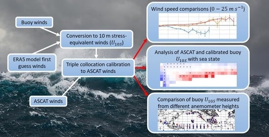
:Buoys provide key observations of wind speed over the ocean and are routinely used as a source of validation data for satellite wind products. However, the movement of buoys in high seas and the airflow over waves might cause inaccurate readings, raising concern when buoys are used as a source of wind speed comparison data. The relative accuracy of buoy winds is quantified through a triple collocation (TC) exercise comparing buoy winds to winds from ASCAT and ERA5. Differences between calibrated buoy winds and ASCAT are analyzed through separating the residuals by anemometer height and testing under high wind-wave and swell conditions. First, we converted buoy winds measured near 3, 4, and 5 m to stress-equivalent winds at 10 m (). Buoy from anemometers near 3 m compared notably lower than buoy from anemometers near 4 and 5 m, illustrating the importance of buoy choice in comparisons with remote sensing data. Using TC calibration of buoy to ASCAT in pure wind-wave conditions, we found that there was a small, but statistically significant difference between height adjusted buoy winds from buoys with 4 and 5 m anemometers compared to the same ASCAT wind speed ranges in high seas. However, this result does not follow conventional arguments for wave sheltering of buoy winds, whereby the lower anemometer height winds are distorted more than the higher anemometer height winds in high winds and high seas. We concluded that wave sheltering is not significantly affecting the winds from buoys between 4 and 5 m with high confidence for winds under 18 ms−1. Further differences between buoy and ASCAT winds are observed in high swell conditions, motivating the need to consider the possible effects of sea state on ASCAT winds.
1. Introduction
High-quality wind speed observations in extreme conditions over the ocean are important to many aspects of meteorology and oceanography. Weather forecasting for the purposes of ship routing depends on reliable observations of winds and waves in conjunction with numerical weather prediction (NWP) to advise ships of adverse conditions along their routes. The availability of reliable winds from remote sensing instruments has advanced the capability of NWP models in this effort, especially winds from scatterometry [1]. Moreover, the forcing of ocean currents with NWP generally relies on calculations of wind stress using wind speed as an input variable and the accuracy of the calculated wind stress values is a function of wind speed accuracy. Bulk formula calculations of wind stress scale with the square or cube of the input wind speeds, depending on the wind speed [2,3]. Therefore, these wind stress calculations are especially sensitive to error at high wind speeds. Applications using bulk formulations of wind stress, such as ocean surface fluxes of momentum, heat, and carbon, rely on accurate winds relative to the ocean surface and are a critical component of characterizing changes in the ocean with a warming climate.
Standard sources of in situ wind data include ships, buoys, and anemometers mounted on platforms such as oil rigs. The availability of observations away from coastal regions is complicated by accessibility for routine maintenance and the harshness of weather conditions in open ocean regions such as the Southern Ocean. For these reasons, remote sensing observations play a prominent role in characterizing winds over the open ocean. Meteorological buoys are a common source of data used for training retrieval functions for remotely sensed ocean vector winds [4,5,6]. The accuracy of buoy winds is complicated by errors which may scale with the wind speed and sea state. These error sources can be either defined by the physical errors inherent to the buoy instruments and platform or errors induced by the environment in which the buoy is located. Physical errors due to the buoy platform include the effects of flow distortion by either the buoy instruments or the platform itself [7]. Environmental errors in buoy wind speed include the near-surface flow distortion over large surface waves [8,9] and the errors due to the pitch and roll of the buoy in high seas.
The movement of buoys in high winds and associated high waves has been suggested to cause problems for the accurate measurement of buoy wind speeds. Buoys may exhibit a low wind speed bias in high winds due to the effects of wave sheltering of buoy anemometers in the troughs of large waves [3,5]. Further non-linear effects may exist in the averaging of winds with the vertical movement of buoys in a logarithmic profile of winds within the near surface boundary layer [10]. The problem with vertical averaging of the wind, is that waves are shaped such that the buoy spends more time in the trough than on the crest of waves, and that a logarithmic profile causes winds in the trough, in the absence of sheltering, to be reduced more than they are increased by an equal and opposite upward motion. Flow over surface waves distorts the notion of a logarithmic wind profile and the wave boundary layer (WBL) is a concern for estimating winds at 10 m from measurements below this height [11].
Traditional techniques used to calculate the wind speed bias of buoys in high winds have not directly accounted for sea state effects, but rather use comparisons of the differences between buoy winds and alternative wind sources at high wind speeds; some of which are uncalibrated [3,5]. To quantify a bias in buoy winds due to sea state, a reference dataset of unbiased observations which are not significantly affected by sea state is needed for comparison. One of the first studies to identify this low bias used buoys with anemometer heights between 3 and 5 m compared to winds from the European Centre for Medium Range Weather Forecasts (ECMWF) operational model to develop linear corrections of buoy winds at high wind speeds based on anemometer height [3]. An alternative study used surface air pressure data with buoys as input into a numerical model to infer a low bias for buoy winds at high wind speeds, but also did not account for sea state effects [5]. There are studies that have used sea state as a factor in comparisons of scatterometer and buoy winds [4], but the results from these studies are limited to the predominant meteorological and sea state conditions of the local area and the physical characteristics of the individual buoys used.
Modern comparisons using buoy data are typically performed with NWP, reanalysis products or remote sensing sources. Scatterometer winds are often compared with buoy winds adjusted to 10 m equivalent neutral winds (). Scatterometers measure electromagnetic backscatter from roughness elements on the ocean surface and are not sensitive to actual winds in the surface layer, but rather the roughness elements sensitive to stress on the ocean surface [12]. Roughness elements at the ocean surface are modified by stability-dependent stress rather than the stability dependent wind profile in the boundary layer. Therefore, comparisons of scatterometer derived winds with in situ winds cannot be soundly achieved without first accounting for the effects of stability. Calculations of equivalent neutral wind account for stability by using a stress and roughness length consistent with the observed atmospheric stratification and then setting the atmospheric stratification term in the modified log-wind profile equal to zero [13,14,15].
Recent work has shown that the measurements from scatterometers have a more direct relationship with surface stress than wind speed because knowledge of the air density improves the match between scatterometer measurements and in situ wind measurements [12,16]. Microwave backscatter from surface roughness elements depends on momentum transferred to the surface water waves, which is affected by both and boundary-layer stratification. Equivalent neutral winds account for boundary-layer stratifications, but not air density. Stress-equivalent winds account for both effects and are calculated using a ratio of to the global mean air-mass density above the ocean ( to convert to .
After comparing scatterometer winds to buoy , variability between ASCAT and buoys can be assessed for possible errors caused by flow distortion and sea state effects, but additional systematic errors due to differences in measurement scales must also be accounted for because we cannot assume that the two sets of observations are perfectly intercalibrated. Implicit assumptions about the errors of a comparison dataset can cause errors in a final calibrated product. Some of the errors that cannot be resolved by dual comparisons include temporal and spatial representation errors, geophysical representation errors, and the error distributions inherent to the individual sources [17]. With dual collocation analyses there is no clear way to differentiate these types of errors introduced by either system. A method introduced by [18] shows when the errors from three separate datasets are uncorrelated, errors may be estimated from the covariances of the three datasets. Triple collocation (TC) allows for the relative linear calibration of the three systems using one type of wind data as the reference system and rescaling the distributions with the estimated errors from mutual calibration [17,18]. While this approach remains sensitive to errors in the comparison data, it does allow for differentiation of the errors from each of the other datasets relative to the comparison data.
This study uses TC with buoy winds from the Global Telecommunications System (GTS), scatterometer winds from the Advanced Scatterometer (ASCAT), and model short range forecast winds used as first-guess (FG) in the ECMWF fifth reanalysis dataset (ERA5) to quantify the effects of sea state on buoy winds in extreme conditions by using ASCAT winds for reference and calculating the linear calibration coefficients of buoy winds under varying high wind and wave conditions. To assess the observational error of buoys at high wind speeds, this study flips the traditional method of using buoy data as “ground truth”. Scatterometer retrievals of wind have been extremely stable over time [19]; hence, they are reasonable to use as comparison data over the life of the missions and scatterometer observations are clearly not sensitive to the physical characteristics of buoys. Scatterometer winds are used as an independent record to test the changes of the observed buoy wind speeds but are not used as a wind standard for gauging the accuracy of the measured buoy winds. This approach does not require that buoy observations or scatterometer winds are correct. It is designed to determine if there is a sea state dependence in the height adjusted buoy winds.
The data are described in Section 2, including the adjustment of buoy and ERA5 FG winds to . The TC error model is described in Section 3. High wind speed comparisons in Section 4 show that buoy performs well when using the full range of winds and seas from all buoys but differs when isolating the statistics to buoys grouped by anemometer height ranges. Sea state comparisons in Section 5 show that knowledge of ocean swell may improve scatterometer wind accuracy and that there appears to be a small dependence of wind speed error on sea state for buoys with anemometer heights ranging from 4 to 5 m. The results section is followed by a discussion in Section 6 and the main conclusions in Section 7.
2. Data
A triple collocation dataset was produced to carry out the work described in this paper using winds from moored buoys acquired through the GTS, ERA5 FG winds, and stable ASCAT winds as the reference system. The ASCAT instrument is a scatterometer carried on the Meteorological Operational (Metop) satellites operated by the European Organization for the Exploitation of Meteorological Satellites (EUMETSAT). For this project, the EUMETSAT Ocean and Sea Ice Satellite Application Facility (OSI SAF) Level 2 ASCAT Coastal Wind product [6,20] on a 12.5-km grid was used with data ranging from 18 August 2010 from Metop-A and 29 October 2012 from Metop-B through 31 October 2019. For the ASCAT instrument onboard both satellites, the geophysical model function (GMF) used to generate equivalent neutral wind vectors based on normalized radar cross-section (NRCS) readings was CMOD7 [21].
The recent C-Band High and Extreme Force Speeds (CHEFS) report from KNMI [11] shows that ASCAT CMOD7 winds show good agreement with buoys at high winds between 15 and 25 ms−1, but lack good GMF calibration due to the lack of a consolidated in-situ wind speed reference for winds above 15 ms−1. The saturation of the GMF at extreme winds (>25 ms−1) is partially compensated by the high calibration stability of the ASCAT instrument. Other studies have examined the quality of ASCAT winds in hurricane force conditions. A recent study comparing ASCAT winds to moored buoys and microwave radiometer winds showed that ASCAT wind retrievals are accurate at high winds up to 25 ms−1, but start to show signal saturation above 42 ms−1 [22]; however, using a different ASCAT GMF. For the purposes of this study, we assessed the buoy wind quality using ASCAT winds below 25 ms−1, where ASCAT winds are shown to be stable, but degradation of buoy wind speed quality may occur. Note that buoy wind measurements above 25 ms−1 are rare and hence, not suitable for statistical analysis.
The in situ wind observations were obtained from buoy data reported through the GTS which are archived and quality controlled by the European Centre for Medium Range Weather Forecasts (ECMWF) [23]. The GTS buoys included in this study are provided by the centers listed in Table 1. The buoy locations are presented in Figure 1. Only buoys moored at least 15 km off shorelines which report both wind speed and direction are used in the TC analyses. The buoy winds are reported hourly by averaging the wind speed over 10 min. Note that many of the GTS buoy winds are binned every 1 ms−1 in speed and 10° in direction due to the GTS buffer message format.
Overall, there are 25 buoys in the anemometer height range shown in Figure 1 centered at 3 m (squares in Figure 1), 155 buoys in the range centered at 4 m (triangles), and 115 buoys in the range centered at 5 m (circles). Buoys with changes in anemometer height and/or hull configurations were treated separately in the analysis. After 2016, the NDBC replaced many of their buoys with anemometer heights near 5 m to buoys with a smaller hull and anemometer at a height closer to 4 m. These buoys are indicated with a star marker in Figure 1. We took advantage of this configuration to test the wind differences of these buoys with different anemometer heights moored at the same locations in the TC comparison results in Section 5. In addition, most of the TAO buoys with the Atlas configuration and hull were replaced with the TAO Refresh configuration during the study period [24] and these buoys were treated separately in the TC analysis.
ERA5 FG winds are used as the third dataset for TC. The ERA5 dataset has a grid spacing of 31 km with winds from 1-hourly forecasts initialized at 06 and 18 UTC [25]. Hourly output of ERA5 FG variables was matched in space and time with GTS buoys by using buoys within the overlying ERA5 grid cell to the closest hourly time. Since GTS buoys report a wind speed average from the last 10 min of each hour, the time difference between the ERA FG and buoy winds were usually within a few minutes. The scatterometer observations from ASCAT-A and ASCAT-B were collocated with buoy data in time and space within 25 km and 30 min (less than half the time of one orbit). Only the closest distance wind vector cell observation within the time and spatial range was chosen for each buoy collocation. With this criterion we have a total of 444,102 triplets. There are instances of matches outside of the ASCAT product grid spacing of 12.5 km but less than 25 km (less than 4.5% of the data). Although in-swath grid spacing for the ASCAT products improved from 25 to 12.5 km, the effective resolution shown by spectral analysis was larger than the grid spacing value [1,26].
Wind Adjustments
The first step in calculating buoy is the conversion of raw winds measured at the buoy anemometer height to buoy . The definition of equivalent neutral winds used for this study follows the conventions [14]. The Coupled Ocean-Atmosphere Response Experiment (COARE) 3.5 bulk model [27] was used for the conversion of raw winds to and the calculation of the friction velocity from both buoy and ERA5 FG winds. The modified log-wind profile is shown in Equation (2) where is the wind at the anemometer height, is the velocity frame of reference (the surface current), is the friction velocity, is von Karman’s constant, is the height above the ocean surface, is the roughness length, is a function of atmospheric stability [28,29], and L is the Monin–Obukhov scale length [30,31].
First, and were calculated using known values of from the buoy, and temperature and pressure from ERA5 which are factored into . The and values were used to calculate using Equation (2) with . was then calculated using Equation (1). In our analysis we assumed a value of ms−1 in the model.
The COARE algorithm parameterizes into two separate terms, with the first based upon the roughness of the ocean under aerodynamically smooth conditions while the second term accounts for the wind stress in the form of surface gravity waves (Equation (3)) [27].
is the kinematic viscosity and is the roughness Reynolds number for smooth flow ( from laboratory experiments [27]). The influences of sea state on are parameterized through the Charnock coefficient (). Based on data from four separate air-sea field experiments with momentum flux measurements, a wind speed dependent form of was calculated where with m−1s and .
Another form includes the parameterization of the influence of surface waves on the ocean roughness with:
where and is the significant wave height. Here, is also a function of the inverse wave age (). is defined as , where (Equation (19)) is the phase speed of the dominant wave, and is the spectral peak period. Since this study involves comparisons of buoy winds against ASCAT under varying sea state conditions, we first tested the sensitivity of the height adjustment of raw buoy winds to using both the wind speed dependent form of and the sea state form as a function of and .
Figure 2 shows scatterplots of ASCAT winds versus buoy derived from the COARE 3.5 model using both the “wind speed only” form of (Figure 2, left) and the parameterization based upon sea state conditions (Figure 2, right).
From Figure 2 it is apparent that the choice of COARE 3.5 parameterization has little effect on the height adjustment of buoy winds with our distribution of GTS buoy winds measured between 3 and 5 m. The correlation coefficient (r), bias (buoy − ASCAT) and standard deviation are closely matched for buoy compared to ASCAT for both parameterizations of . Although the changes in are important to consider for fluxes, the height adjustment of wind speed is rather insensitive to roughness length. The results in Section 5 were also tested with the wave age formulation, but they were not visually different from using the wind speed formulation. For simplicity, we chose the wind speed-dependent formulation in the COARE model for further analysis.
The distribution of buoy for each anemometer height used in the analysis is shown in Figure 3. Wind observations from buoys with 5 m anemometers were readily available for all wind ranges. The median observations of buoy from 4 and 5 m anemometers aligned well, but there was a higher occurrence of high with 5-m anemometers compared to 4- and 3-m anemometers. More buoys with 5-m anemometers were in the mid-latitude regions than buoys with 4- or 3-m anemometers and there was a more frequent occurrence of high winds in the mid-latitudes. The median values of buoy from 3 m anemometers was lower than for 4 and 5 m anemometers. Most of the 3-m observations were from the RAMA array in the Indian Ocean, and there is a more frequent occurrence of light winds in this region. The narrow PDF of 4 m buoy winds with the median winds near 6–7 ms−1 reflects the fact that most of these winds are from the TAO, PIRATA, and RAMA arrays in the tropical region where steady trade winds dominate the climatology. There is a much lower occurrence of high winds (greater than 10 ms−1) for buoys with anemometers near 4 m. The non-uniform nature of global winds combined with the steepness of the 4 m buoy PDF between 7 and 10 ms−1 is indicative of conditional sampling of winds at point locations where the wind climatology varies with latitude.
If the wind record of buoys around 4-m anemometer height were combined and compared to the wind record of 3- and 5-m winds, we may see an artificial bias in the 4-m buoy winds between 7 and 10 ms−1 due to the different distributions of wind speeds. Since the buoy wind climatologies vary with location the differences are expected, and the technique to assess differences associated with height adjustment must be robust to these different distributions. This will be accomplished by using only collocated observations with ASCAT in space and time. The buoy wind calibrations in the following sections are not performed on groups of buoys based on anemometer height, but rather the calibrations occur at the individual buoy level.
3. Buoy Validation Parameters
In this section, we determine the parameters to validate the buoy winds using the TC model first introduced by Stoffelen [18]. This approach considers errors in both the buoy winds and the reference ASCAT winds. Through this approach, we determined improved bias and standard deviations for the triple collocated data.
This procedure was applied to ASCAT-A and ASCAT-B data generated with the CMOD7 GMF [21]. ASCAT winds have been shown to be stable over time and therefore justified as a reference to test the buoy error dependency on sea state [1,19,32]. Instead of applying the TC on the entire buoy dataset, we first applied the procedure at the individual buoy level. The buoy dataset included buoys with many different physical characteristics such as different hull designs and instrument heights and are reported through the GTS by different organizations with their own calibration standards and quality control methods [23]. Performing TC at the individual buoy level more effectively isolates the error sources unique to the individual buoys. After the procedure was complete, buoys were grouped by anemometer height for an analysis of the residuals between the calibrated buoy and ASCAT winds and tested against sea state variables.
Triple Collocation
For a full discussion on the triple collocation error model, the reader is referred to [17,18,33,34]. We had three measurement systems () measuring the “truth” value () for , and if we assumed linear calibration suffices, then the measurements would satisfy the following set of equations where and are the linear scalings and bias calibration corrections relative to , and is the random error of system .
From this system of equations, we can derive the error variances based on the assumption that the random measurement errors are not biased (, where denotes the average). Calibration and wind retrieval errors often result in systematic wind speed errors and can be detected in wind speed comparisons alone. On the other hand, 3D turbulence and the different spatial and temporal aggregation in in situ, satellite, and NWP model winds provide, inherently, a vector nature to wind velocity differences [35]. When comparing different error sources, wind speed components, rather than magnitude and direction, have a more symmetric error distribution and are easier to describe with the linear TC model. Therefore, we performed the TC calibration on the u and v components of the three wind datasets instead of the wind speed magnitude. There are additional assumptions that must be satisfied to perform TC using the error model of Equation (6). The measurement errors must have constant variance over the whole range of measurement values and, except for spatial representation errors, must be uncorrelated with each other. The mixed second order moments relating the calibration factors are shown in Equation (7).
If system 0 and 1 have a better spatial resolution than system 2, they both may resolve actual wind variance not resolved by system 2. This representation error variance (r2) is part of the wind variances for systems 0 and 1 given as the covariance of the observation errors with TC (). In our example, since both ASCAT and buoys had better spatial resolution than ERA5, they both may have resolved true wind variance that is not resolved by ERA5 and is accounted for in the TC model. The calculation methods are discussed in following paragraphs.
The calibration scalings (slopes associated with errors in proportionality) are given in Equations (8)–(10) based upon different scenarios for choosing a reference and the assumption that system 2 has a coarser spatial resolution than both systems 0 and 1. The bias corrections are given by Equation (11), where is the 1st order moment of system i.
The calibrated datasets are created by:
As seen in Equations (8)–(11), has a direct influence on the calibration scalings () and the bias correction factors (); thus, care must be taken to separate and properly characterize these systematic and random errors. Methods to calculate typically involve using the difference of the power wind spectra of collocated scatterometer and coarser resolution model winds [36]. Another method was to calculate the cumulative variance of scatterometer and model winds as a function of scale and is found by taking the difference in cumulative variance between the scatterometer and model at the scale of the coarser model resolution [37]. By spatially analyzing the difference between scatterometer and model winds, the spatial content of the common variance t in Equation (6) can be further analyzed [38]. Both methods require series of wind data representative of global conditions across the ocean. Since our TC dataset includes observations which may be highly variable and localized, we sought an alternative method to compute .
Following the examples of [34,39], we performed TC using the coarsest measurement (ERA5 FG ) as the standard and repeat TC with different values until optimal intercalibration was reached. This is akin to using system 2 as the reference in the TC equations. The values for u and v that determine a wind speed magnitude bias close to zero () for the calibrated triplets were considered the best-estimated spatial representation error variance. To achieve this, we performed TC using the entire dataset and test different combinations of and until the aforementioned bias was approximately 0. The ratio of and for stable winds found using classical wind spectra based TC as defined by [36] is /. We took advantage of this ratio to simplify our search for the optimal values. For the overall TC dataset, we found that and m2s−2. These values are lower than many previous calculations of representation errors [21,34,40,41], but are reasonable given the small effect of and on the final results. We used ERA5 as the reference dataset for the calculation of and only. For the main analysis, TC was performed for individual buoys using ASCAT as the reference dataset with and m2s−2.
4. High Wind Speed Comparisons
For the purposes of this study, we defined low winds as winds less than 5 ms−1, moderate winds being between 5 and 15 ms−1, and high winds being between 15 and 25 ms−1. Above this range we considered extreme winds (>25 ms−1). No statistically significant sample of winds >25 ms−1 have been measured by buoys. In this section we show comparisons of winds less than 25 ms−1, with a focus on winds in the high wind speed category. As a first test, we compared the height adjusted buoy winds to ASCAT prior to calibration for comparison of wind speed magnitude in the high wind ranges. Figure 4 shows the comparisons of winds grouped by anemometer height and wind speed ranges based on the average of ASCAT and buoy .
The raw winds from the different anemometer heights (Figure 4, top) followed an expected pattern with higher winds from 5-m anemometers compared to 4- and 3-m winds in the same ASCAT wind speed ranges. The height adjustment to brought the winds closer together (Figure 4, bottom), but unexpectedly, there was still an organized separation with 3-m winds much lower than the 4- and 5-m buoy residuals for winds above 7.5 ms−1. For buoys with anemometers near 4- and 5-m, buoy was closely matched for the ranges shown in Figure 4, but both groups of buoy winds were above ASCAT for winds greater than 15 ms−1. Table 2 shows the same wind characteristics as the bottom panel of Figure 4, but the winds were grouped into 5 ms−1 ranges and it also provided the averages for each range using the entire buoy dataset. The high standard deviations for buoys with 2.5 to 3.5 m anemometers above 15 ms−1 reflects the lack of observations above this range and there was high uncertainty in these values. Nevertheless, the separation of buoy measured near 3 m with buoy measured near 4 and 5 m shows that the choice of buoys is an important factor in remote sensing comparisons.
Most of the high wind speed observations above 15 ms−1 are from buoys with anemometers near 5 m as shown in the PDFs of Figure 3. Even with the higher availability of 5-m winds, the standard deviation of the wind residuals in the 20–25 ms−1 range was greater than the standard deviation of buoy measured near 4-m anemometer heights, although the biases were the same with buoy winds higher than ASCAT by 0.73 ms−1. Given that there was a much larger sample of winds measured near 5 m compared to 4 m above 20 ms−1, we expected that the high variability in the residuals was driven more by the large variability of winds in the mid-latitude regions, corresponding to the location of most of the 5-m anemometer buoys shown in Figure 1.
The CHEFS report by the Royal Netherlands Meteorological Institute [11] showed a bias of 0.3 ms−1 for winds between 15 and 25 ms−1 (15 ms−1 < (ASCAT + buoy )/2 < 25 ms−1, N ≈ 9700) and a standard deviation of 1.27 ms−1 using the same buoy and ASCAT dataset, but not the exact same observations. If we make the same comparison using our data for the same range (15 ms−1 < (ASCAT + buoy )/2 < 25 ms−1, N ≈ 6674), we find a similar bias of 0.34 ms−1 with a standard deviation of 1.20 ms−1. However, if buoy is used, we find a slightly higher bias of 0.41 ms−1 with a similar standard deviation of 1.19 ms−1. It is apparent that the choice of buoys with different anemometer heights can significantly affect the overall statistics given the drastically different biases shown in Figure 4 and Table 2, and from the perspective of determining long-term trends, or return periods of extreme winds, this result indicates that changing buoy heights could have an impact on these statistics.
Several geophysical effects may lead to differences between buoy and ASCAT winds. Large wind variability in the extratropics and the effects of currents in the tropics are shown to affect buoy wind comparisons [16]. To isolate the error sources more effectively to the individual buoys and their locations, we performed TC at the individual level. Figure 5 shows the calibration scalings () for the buoy wind components calibrated using ASCAT as the reference winds. The calibration scalings were used in conjunction with the bias correction terms (, Figure 6) to linearly correct buoy towards ASCAT. The biases were simply the average differences between the datasets (Equation (11)). The combination of the scaling () and the offset () can be used to determine ranges over which an instrument overestimates or underestimates relative to one of the other datasets (Equation (12)). These were exactly analogous to changes in a line due to a regression of the slope and y-intercept. The key difference in concept is accounting for similarity in the sub-gridscale variability in two of the datasets relative to another when determining the slope (Equations (8)–(10)).
From a visual inspection of the buoy calibration scalings in Figure 5, we observed some areas with patterns in the calibration components. In the tropics, there is a large variation in and values with the TAO array. Given that all the TAO buoy winds are measured from a height of 4 m, this variation in wind components seems to not be systematically related to the anemometer height, but rather geophysical effects in this region. In the western tropical Pacific, the v-components for were nearly all positive and there was a large variation in the v-components for . Before calibration, most of the v-component wind values with the TRITON buoys were below ASCAT values for the entire wind range. Another area of interest is off the Pacific Northwest coast of the United States, where values for both u and v components are consistently less than 1. This is an area that experiences strong upwelling of cold water during the northern hemisphere summer.
It is important to note that sampling and the appropriateness of the TC error model determines the accuracy of the result [41], and individual buoy calibrations are subject to conditions local to the respective buoy area. The ERA5 variability and variability deficit depend on local conditions, particularly near the equator where both the root-mean-square deviation and bias change sharply with latitude [42]. The inter-tropical convergence zone moves over a year and hence the speeds, variability conditions, and errors at most tropical buoy locations change systematically over the year. This may violate the assumption of constant bias and random error as a function of speed. Most of the buoys in the 3.5–4.5 m anemometer height range are located in the trades and have a rather narrow dynamic range, which makes the results on the error estimates rather uncertain as distinction between and values is poor. This is important to consider with the given distribution of and values shown in Figure 5 and Figure 6. With the given caveats in the TC methodology, we did not observe any strong trends between the anemometer height ranges and the calibration components from Figure 5 and Figure 6 alone, but rather differences due to possible geophysical affects for specific areas.
Table 3 shows the average and standard deviation of the wind component residual biases for calibrated buoy and ERA5 FG grouped by anemometer height bins. Overall, the calibrated ERA5 FG and buoy wind components compare favorably with ASCAT for all anemometer height bins with low bias for each bin. The pattern of standard deviations from ERA5 FG winds and buoy are similar, where the standard deviation of components from buoys in the 3.5–4.5 m bin are smaller on average than the other two wind height bins. This again may reflect that the overwhelming number of buoys with anemometers near 4 m are in the tropical trade wind regions. Buoys in the 2.5–3.5 m bin appear mainly in tropical moist convective regions, hence the low winds and high variability.
In the following section we provide evidence that the differences in the calibrated residuals are intricately linked to the local sea state; therefore, we do not draw a conclusion about these biases in this section, other than that they are small when grouped as a whole. Since TC is performed at the individual buoy level, the calibration of each buoy to ASCAT is dependent on the dominant conditions of the local region. The following sections helps to contextualize the observed differences in the comparisons with ASCAT for buoy winds calibrated under different conditions. Since the interpretation of wind speed magnitude comparisons are easier understood than comparisons with individual components, we converted the calibrated u and v buoy components into wind speed magnitude for comparison with ASCAT in the following section.
5. Residual Analysis with Sea State
Sea State Comparisons
There are many ways to describe sea state [43,44,45], and the easiest to visualize is that wind-waves tend to be steeper, with a greater ratio of wave height to wavelength, while swell are more gently sloped. Swell waves can have quite large amplitudes, but they have longer wavelengths resulting in smaller slopes. The sea state parameters described herein are all derived from ERA5. The ERA5/ECMWF wave model used for the separation of wind-waves from swell is described in [46]. One of the output parameters at each ERA5 grid point is the two-dimensional wave spectrum, . The wave spectrum describes the distribution of wave energy as a function of frequency (, which is related to the wavelength via the dispersion relation) and wave propagation direction (). The spectral components subject to wind forcing are delineated by Equation (13), where is the wave phase speed (as a function of wave frequency) and is the wind direction. To a good approximation, waves are still subject to wind forcing when [46].
The moment of order n for , is defined by Equation (14) and the definition of significant wave height is shown by Equation (15). The zero-moment of Equation (14) () is the mean variance of the sea surface elevation [47].
is the significant wave height when the integral in Equation (14) is performed over all components of the spectrum. It is a statistical quantity of the wave field that roughly corresponds to the average height of the highest one-third of waves (trough to crest). By extension, the wind-wave significant wave height () is computed by only integrating Equation (14) over the components of that satisfy . For the purposes of our study, wind seas were classified with . The mean wave direction () was derived from the full 2-dimensional wave spectrum [46]. Swell and mixed seas were defined by and we delineated mixed seas and swell dominant conditions using the squared fraction of ERA5 and ERA5 in Equation (16).
If was at least twice the height of ( greater than 4.0), then we defined the sea state as swell dominated. In between values of 0.25 and 4.0 we defined a sea state of mixed wind-waves and swell. alone may not provide enough information on how either the buoy or ASCAT winds are affected by sea state. For this reason, we investigated the relationships between common sea state parameters and the calibrated wind residuals (buoy –ASCAT). The integral wave steepness is defined in Equation (17), where is the mean wavelength and is the mean wave period. Peak wave period () differs from in that represents the period of the waves with the highest energy versus which represents the weighted mean of all wave periods in the spectrum. The calculation method of and from the full 2-dimensional wave spectrum in the ERA5 wave model is given in [46]. Wave orbital velocity ( is defined in Equation (18) using and the wave phase speed () is shown in Equation (19). It has been theoretically demonstrated that straining of shorter waves by the orbital motion of the longer waves contributes to the steepening of the gravity waves [48] and consideration of orbital velocity leads to drag coefficient formulations that are in better agreement with experimental results [49,50]. Here, we did not define where the mean wave direction is in-line with or against the wind direction, but instead used the simple relationship shown in Equation (18) for all conditions. The correlations between the wave and thermal parameters calculated with ERA5 and the calibrated wind residuals are shown in Figure 7.
From Figure 7, the strongest correlations with the calibrated residuals occur with ERA5 air temperature and sea surface temperature (SST). Compared to Ku-band scatterometers, SST effects are shown to be much smaller at C-band frequencies (ASCAT) and are wind speed-dependent [51]. Since this study is concerned with the possible effects of wave sheltering of buoy winds, it is important to isolate the error sources which may confuse the interpretation of the buoy wind speed differences under high winds and waves. Here, we continue with the analysis of the residuals with sea state, but also examine the effects of SST on the residuals.
All of the sea state variables shown in Figure 7 are nearly independent from the wind speed residuals with extremely low correlations. shows a correlation near 0. However, we noted that the correlation may change when the conditions are limited to wind and wave directions that are nearly aligned. and have correlations close to zero, showing that the wind speed differences between ASCAT and buoys are not best described by a linear function of wave height alone. In fact, Figure 7 shows that the mean wave period is better related to the distribution of calibrated wind residuals than wave height. and have weak and opposite correlations. The calculations of and both include wave period and are traditional indicators for defining the sea state [44,49,52,53]. As increases, the sea state is more defined by wind seas than swell [45]. Here, we observed a positive correlation of the calibrated wind residuals with with the trend where either buoy increases in reference to ASCAT or ASCAT winds decrease in reference to the buoys as the sea state moves from more swell dominated to wind-wave conditions. The negative correlation with supports this idea given that large values are associated with swell dominant conditions. We observe a smaller correlation to than [54] and noted that their correlations with were dependent on the incidence angle of the wind readings. In addition, we noted that using either buoy or ASCAT winds in the formulation of in the calculation led to a larger correlation with the calibrated wind speed residuals, and we observed a similar correlation as [54] when using buoy winds in our formulation (not shown). We only used ERA5 model first-guess winds in our calculation to avoid a spurious cross-correlation.
These cases show that sea state was related with the distribution of wind speed residuals for sea state variables derived from and , but the relationship was weak when looking at individual correlations alone. Figure 8 shows the results of comparing the calibrated wind speed residuals (buoy –ASCAT) to with sea state defined by wind seas (), mixed seas () and swell (). The first noticeable trend is that the calibrated buoy values for swell dominated seas were below ASCAT and calibrated buoy values for wind-waves are above ASCAT. Unlike the swell dominated residuals, the wind-wave residuals did not strongly decrease with increasing . Swell conditions showed the strongest variability in the given range. To within uncertainty in these biases, the calibrated wind speed biases for mixed seas were usually between the residuals from the wind-wave and swell dominated seas. For the most part, these differences greatly exceeded one standard deviation of the random uncertainty, i.e., tended to be statistically significant.
As seen with the relatively low correlation in Figure 7, alone was not a great indicator of the differences between calibrated buoy and ASCAT. Since is a traditional indicator of sea development [27], we investigate how the residuals change combining both and in Figure 9. This figure shows that changes in both and were strongly related to the differences between buoy winds and ASCAT, and that these differences varied in a well-defined pattern. Young seas with a small wave age below 30 were generally associated with calibrated buoy above ASCAT wind speeds, while old seas with high and high were associated with ASCAT winds higher than calibrated buoy .
To have confidence in the results from Figure 8 and Figure 9, we also had to isolate possible effects on the ASCAT winds due to SST since SST had the highest direct correlation with the wind speed residuals (Figure 7) and varied with latitude and wind speed conditions. In Figure 10, we tested the calibrated residual (calibrated buoy –ASCAT) in relatively high seas with between 4 and 6 m and binned by both SST and ranges. We chose this range as it is where we observe the largest changes in the residuals from low to high in Figure 9. A shift of the entire PDF along the x-axis of Figure 8 would correspond to a change in the mean residuals, indicative of a dependency of the residuals on the variable in question. For SST, all categories of residual had the same bias, until SST exceeded 24 °C, at which point there was a small observable shift in the negative direction. There was a slightly more noticeable shift in the mean residuals with changing values of , where the residuals moved in the negative direction as increases. The same was true with increasing wind speed, where the residuals moved in the negative direction as ERA5 FG increased. The dependency of the wind speed residuals in this range was more sensitive to and ERA5 FG rather than SST, giving confidence that the large wind speed residuals in Figure 8 and Figure 9 are not due to shifting SST.
Since the value in was also derived from ERA5 FG winds, and has a direct relationship with wind speed [27], the PDFs in Figure 10 show a contrasting effect where increasing (and increasing ) is associated with a negative shift in the residuals (calibrated buoy decreasing w.r.t ASCAT), but increasing ERA5 FG also is associated with the negative shift, but decreasing . Therefore, the strong negative residuals with high and high were associated with light winds or long wave periods. For the same range between 4 and 6 m, if we averaged and into bins, we found that with increasing there was a more drastic decrease in compared to an increase in (not shown). Where we observed the significant negative residuals in Figure 9 with between 4 and 6 m and between 70 and 170, the average ERA5 FG value was a moderate 6.9 ms−1, while the average value was 14.1 s (with 22 ms−1) and an average value of 0.23 ms−1. Although the residuals were more sensitive to changes in compared to , we observed significant differences between calibrated buoy and ASCAT even at moderate winds speeds under these conditions. This example shows the differences with sea state are not only isolated to the extreme low and high wind speed ranges.
It is worth mentioning at this point that the TC calibration may affect the interpretation of these results. The residuals were statistically biased due to conditional sampling of high ERA5 winds in the given range between 4 and 6 m. Since SST has a strong relationship with changes in latitude, the calibrated buoy winds were influenced by changes in and values in this direction. and had a strong relationship with changes in longitude, and, hence, were affected by the changes in shown near the coast in Figure 5. Although calibration of the buoy winds reduced the overall bias with respect to ASCAT, it is important to consider how this may affect the results when limiting the sample to a range smaller than which the calibrations took place. Overall, TC calibration at the individual buoy level reduced the differences between ASCAT and the buoy winds (shown in Figure 8 and Figure 9) compared to TC calibration using all buoys (not shown). This gives confidence that TC at the individual buoy level is appropriate for use for the sea state comparisons shown here.
In the cases shown in this section, the TC calibration was not independent of the dominant sea state for the individual buoy locations. For example, if the 4-m buoys were in an area dominated by swell conditions for most of the timeseries, then the calibrated residuals for swell would be less than other buoys that were not in swell-dominated conditions. Organizing the residuals in this way does, however, give statistical evidence of the possible problems associated with either ASCAT or the buoys with the dominant sea states. To further isolate the differing effects of swell and wind-waves, we performed TC calibration at the individual buoy level explicitly using cases with wind-wave-dominated seas while still holding ASCAT as the reference dataset.
Wind-Wave-Dominated Seas
It has been established that the wind-wave portion of the wave spectrum that dominates the magnitude of the wind stress is directly affected by large gravity waves [55,56,57,58]. Our results up to this point indicate that wind stress might be affected by the presence of swell in addition to large wind-driven gravity waves and further investigation is required to separate the possible sea state effects on buoys versus the scatterometer winds. Here we again performed TC with ASCAT as a reference at the individual buoy level but isolated the observations to the predefined wind-wave conditions () using buoys which have at least 250 triplets under these conditions. This limits the collocated data to 13% of the original triplets corresponding to 82 of the original 295 buoys. Of these, only 2 of the buoys have anemometers with a height near 3 m and 13 have an anemometer height between 3.8 and 4.1 m. There was a much larger sample of 66 buoys with anemometer heights near 5 m. For this reason, we chose to base our comparisons in this section on winds from anemometers near 4 and 5 m. Performing TC in this manner allowed us to isolate possible wave flow distortion effects in high winds and associated wind-driven waves while limiting the swell effects illustrated in the previous section.
We tested the buoy winds measured from anemometers between 3.6 and 5.1 m to quantify the differences between calibrated buoy and ASCAT for different ranges of wind speed and (Figure 11). By taking the mean wind speed residuals from buoys with anemometers near 5 m and subtracting the mean residuals from buoys with anemometers near 4 m, we observed how increasing wave height and wind speeds contribute to buoy wind speed error relative to ASCAT. From Figure 11, there is not a strong trend in the differences of the residuals increasing with increasing wind speed and wave height until we reach above 4. We observe significant differences between the mean buoy residuals with between 4 and 5 m and ASCAT wind speeds between 12 and 18 ms−1. The significant differences between the residuals are negative in this range, indicating that calibrated buoy from anemometers near 4 m is generally greater than calibrated buoy from buoys with anemometers near 5 m under these specific conditions.
This finding is the opposite of what we would expect from previous arguments of wave sheltering, where winds measured from a lower height should compare lower to a reference in high winds and waves compared to winds from a higher anemometer [3]. If the wind profile is assumed to be close to logarithmic near the surface, we would expect to observe larger differences between 4 m anemometer height residuals as high waves may effectively lower the winds from lower anemometer heights more than higher anemometers compared to the wind reference. It is worth pointing out that the uncertainty in the differences of the binned residuals with above 4 m noticeably increases, but within the uncertainty bounds we do not observe a large separation between the residuals measured from the different anemometer heights. Our results in Figure 11 support the argument that wave sheltering is not a significant contributing factor to buoy wind speed error for winds measured at 4 and 5 m in the given ranges below 21 ms−1.
For a comparison of the calibration coefficients in wind-waves we plot the and values for the u and v components of the buoys with reference to ASCAT (Figure 12 and Figure 13). Compared to the values for the u-component calculated with the full range of winds (Figure 5, top), there is a more systematic change for values from the u-component in wind-waves only. South of 20°N the u-component values are all negative, and the majority of u-component values are positive north of 20°N. We can only speculate on the cause of the buoy and ASCAT differences in the u-component of the winds with latitude; however, since the sample is mixed with buoys that have anemometers near 4 and 5 m, we suggest that this change is not likely to be due to the physical characteristics of the individual buoys. Although our calibration was performed at the individual buoy level, a similar pattern was found in a study using global TC where the different errors in u and v of ERA5 are the main cause [42]. We did not observe a similar shift in the v-component values with changing latitude, but do note that many of the v-component values off the eastern coast of the United States are below 1 and u-component above 1, suggesting that many of the buoys underestimate the u-component and overestimate the v-component off the eastern United States and in the Gulf of Mexico. Compared to the values, there was less of an observable pattern in the values shown in Figure 13.
Since there are systematic changes in the values with latitude, a comparison of the wind calibration coefficients averaged together are skewed given that the distribution of buoy anemometer heights is also not consistent with latitude. In addition, the distribution of buoys with anemometer heights near 4 m are located further offshore than many of the buoys with anemometers near 5 m. This could affect the TC statistics given higher wind variability in the near coastal regions [34]. However, there are instances where the NDBC buoys changed from anemometers near 5 m to anemometers near 4 m in the same location. Of the 14 buoys in the 3.5 to 4.5 m anemometer height range that met the minimum number of triplets under the wind-wave criteria, 5 of the buoys have separate calibrations before and after a change from approximately 5 to 4 m. Since these buoys were in the same general area before and after the switch, we can directly compare the calibration coefficients to investigate any trends before and after the changes. Table 4 shows the calibration coefficients of these stations.
From this subset of 5 stations, there is not a strong trend of changes the calibration coefficients from the 5 m anemometer height buoys to the 4 m wind height. The a values do not strongly change from the higher to the lower anemometer height. The average of the differences for and from 5 to 4 m height are −0.012 and −0.0328, respectively, with standard deviations of 0.042 and 0.067. The standard deviations are both higher than the averaged differences between the scalings for the two anemometer heights. The averaged differences in the bias terms are a bit larger with the differences being −0.086 for and 0.198 ms−1 for with standard deviations of 0.29 and 0.38 ms−1. With the low sample of buoys and high standard deviation of the component differences relative to the averages, we cannot decisively show any real overall trends with the component differences for the buoys with changes from 5 and 4 m anemometer heights. This again supports the argument that wave sheltering is not a significant contributing factor to buoy wind speed error for winds measured at 4 and 5 m given the small sample of buoys and wind conditions shown here.
6. Discussion
Wind observations from buoys with many physical differences were used in this study. The buoys are generally either aluminum or foam discus buoys with anemometer heights between 3 and 5 m. The error characteristics were divided by anemometer height, but there may also be errors due to differences in hull type and flow distortion around the anemometer. Other differences in the observed winds may be due to different calibration practices from organizations reporting the buoy observations to the GTS. From the results shown here, the differences in buoy and ASCAT winds may be influenced by sea state, especially with high and large or small values relative to the value for local equilibrium. Here, we summarized our findings of how sea state may play a role in the differences in buoy and ASCAT and contrast this with other possible error sources and give explanations on possible ways the noted results may be statistical rather that physical.
6.1. Sea State Errors
6.1.1. Wind-Wave Flow Distortion
Our analysis of calibrated wind speed residuals in wind-wave-dominant conditions for buoys with anemometers near 4 and 5 m shows a minor separation between the average wind residuals in high wind-waves, but the differences between the calibrated residuals do not follow the expected pattern where the wind from 4 m buoys is distorted more than the wind from 5 m buoy in high winds and seas. We expected to observe higher flow distortion with winds measured closer to the ocean surface given previous arguments of wave sheltering [3]. Our results indicate that there is a larger difference with calibrated buoy and ASCAT winds for buoys with anemometers near 5 m compared to a smaller difference between calibrated buoy and ASCAT winds for buoys with anemometers near 4 m for between 4 and 5 m and ASCAT winds between 12 and 18 ms−1 (Figure 11). The uncertainty of the observations drastically increases with increasing wind speed for pure wind-waves, especially with winds over 18 ms−1. This analysis assumes that both ASCAT and ERA5 are a good reference to test the buoy winds against. The physics for deriving the scatterometer winds from ocean surface roughness elements does not depend on anemometer height, but the TC calibration of buoy winds to ASCAT may depend on predominant local conditions and TC assumptions.
With these considerations, we concluded that wave sheltering is not significantly affecting the winds from buoys with 4 and 5 m anemometers with high confidence for winds under 18 ms−1. Compared to [3], the averaged differences between buoys with 4 and 5 m anemometers using ASCAT as the reference were much lower than the differences between the CASID buoy with a 3-m anemometer and NDBC buoys 46,004 and 46,005 with 5-m anemometers using ECMWF model winds as the reference dataset during the Ocean Storms Experiment. The results shown here compare favorably with [8] and illustrate that buoy wind speed errors possibly due to wave sheltering are smaller than other sources of error at high wind speeds such as platform flow distortion [7]. It is unfortunate that the sample of buoys with anemometer heights near 3 m in wind-wave conditions was too small for the TC analysis. It is expected that wind-wave flow distortion would play a larger role in the accuracy of winds measured from lower anemometer heights given the nature of the logarithmic wind profile in the boundary-layer. Although our results indicate that there is little difference between buoy with buoys anemometer heights near 4 and 5 m in high wind-wave conditions, we cannot rule out that wave sheltering is not a factor in the accuracy of winds measured from buoys with anemometers below 4 m.
6.1.2. Swell Wave Effects
Compared to pure wind-waves, the observed differences between ASCAT and buoy are larger in scale for pure swell conditions in high seas (Figure 8), although the differences may not be due to alone. NRCS SST dependencies have been evaluated as rather weak for C-band scatterometry [51], but direct correlations tend to be more noticeable than those to sea state (Figure 7). This is probably due to the fact that SST correlates with climate zones and their varying geophysical conditions and wind variability. SST gradients have been shown to have a profound effect on wind variability and hence buoy and scatterometer collocation errors [42,59]. Refinement of our analysis revealed that SST changes were not a large factor on the wind speed residuals when isolating conditions to where we observe the largest differences between calibrated buoy and ASCAT in Figure 9. We illustrated that the shifts the largest residuals were associated with shifts in when isolating between 4 and 6 m. We also observed that the shifts in the were due more to shifts in than . The combination of high and moderate-to-low was connected to ASCAT winds consistently above buoy . Evaluating covariance of these variables may provide a good indication of causation, but all other true conditions should remain the same ideally, which does not tend to happen. It is also important to consider how wind PDF and variability with the given distribution of buoy winds may affect the comparisons. For example, wind variability broadens the buoy wind speed PDF and hence may cause pseudo biases and errors in proportionality when comparing to scatterometer winds [18]. Further tests may be needed to estimate the dominating factors at play.
The steady decrease in wind speed residuals with increasing swell and the lack of separation between 4 and 5 m anemometer residuals provides a suggestion that this problem is not related with the buoy wind speed error. Scatterometer readings are sensitive to roughness elements caused by stress on the ocean, and there are multiple field experiments [55,56] and models [49] indicating stress decreases with swell compared to wind-waves. There are relatively few studies that have directly documented ASCAT wind error with swell waves. A neural model developed by [52] for the C-band European Remote Sensing Satellite (ERS2) scatterometer related the NRCS to both surface wind and sea state information and found a marginal impact by swell waves on the NRCS and related this error to significant wave slope. The correlation they found was that NRCS dependencies on sea state reduce with increasing incidence angle, but given the larger noise in ERS winds, no causation seems implied. A study by [60] found that a variety of swell parameters significantly influenced the radar cross section of the ERS-1/2 scatterometers in a manner that led to overestimation of the wind retrievals. A more recent study by [54] using buoy wind comparisons to ASCAT winds from the CMOD5.N GMF also confirm that low frequency swell causes overestimation of ASCAT winds measured at low incidence angles in reference to NDBC buoys. Wind retrievals based on CMOD5 have documented vector-dependent biases which are dependent on incidence angle and change across the swath. Therefore, a change in vector distribution in the across-track wind vector cells (WVCs) may cause biases and drifts in the derived ASCAT winds. This problem was significantly improved with development of the CMOD7 GMF [21], although our results show there could still be room for improvement.
Ocean swell modifies the surface roughness spectrum by tilting the surfaces over which capillary waves ride, and therefore, influencing the angle at which emitted backscatter from the satellite encounters the surface roughness elements which affects the returned signal strength [61]. The extra tilting may contribute to a larger signal variation of scatterometer measurements and modification of the wind speed dependence of the NRCS [52,54,61]. The signal increase due to the non-linear incidence-angle dependence would result in higher for higher swell for fixed ocean stress conditions. One may expect to see higher slope modulation effects in high wind-waves, but our observations surprisingly show that the effect is most pronounced in high swell with large wave ages associated with long wavelengths and hence low surface slopes (Figure 9). The inclusion of incidence angle (across-swath WVC number) as shown by [52,54,62] with estimates of and may help to further refine the conditions under which the tilting effects are most pronounced. This is especially important with the planned launch of the EUMETSAT Polar System-Second Generation Satellite B in 2022 with a C-band scatterometer having a lower minimum incidence angle compared to ASCAT [63].
Another possible explanation is that non-linear wave–wave interaction is contributing to the amplitude of Bragg scattering waves [64]. This mechanism is controversial [58] and likely to be overestimated in [64]. However, it is plausible that swell acts to damp the magnitude of short gravity waves and the gravity-capillary waves that cause the Bragg scattering. This explanation has the advantage of explaining the systematic errors seen for the small wave ages observed with rising seas but does not explain why we observe ASCAT winds above the buoys in areas of high swell.
It is important to note that these are just a couple of possible explanations for the comparison results shown here in areas of high swell. The subject of this paper was a test of how buoy winds are affected in high winds and seas and a more thorough investigation of ASCAT winds should be undertaken. It is possible that the impact of sea state is more pronounced on the NRCS values from the three individual beams of the ASCAT before they are merged and used with the scatterometer GMF [54]. An analysis with the ASCAT maximum likelihood estimator (MLE) winds would be beneficial for a fundamental understanding of how sea state may impact scatterometer winds and is suggested for future work.
6.2. Other Sources of Comparison Error
In addition to errors in the comparison of ASCAT and buoys due to sea state, other error sources must be considered that influence the comparisons in high wind conditions. By using buoy , we accounted for the possible effects of air mass density and to better match buoy and ERA5 winds with ASCAT. Even with these considerations other factors may lead to some of the observed differences we find in this study.
6.2.1. Platform Airflow Distortion
Another possible source of error is with flow distortion of the air with the buoy platforms and instrument packages. Even though a full investigation of the flow characteristics is outside of the scope of this study, recent studies have used novel techniques to characterize the effects of flow distortion on buoy wind speeds. The directional pattern of inter-anemometer disagreement for buoys with dual anemometers from the Woods Hole Oceanographic Institute and comparison to ASCAT to characterize flow distortion by the buoy platform and instruments was calculated by [7]. They found that the disagreement between the anemometers can be up to 5% due to flow distortion. Occasionally, these differences can contribute to errors of ±1 ms−1 at 20 ms−1. These errors are of a similar magnitude as the observed wind speed differences from our analysis. Many buoys do not report a heading as with [7], but for a full investigation of buoy wind speed error, flow distortion by the instrument platform must be considered.
6.2.2. Triple Collocation
An investigation of multiple collocation methods is shown by [41] who summarize benefits and limitations. TC regresses three datasets simultaneously with a set of assumptions, captured in an error model, common to the three systems compared. TC is amended by assumptions on spatial representativeness. Where the error properties of buoys, ASCAT and ERA5 are all different, the behavior of each of them with respect to the error model assumptions may affect the TC results of all three systems, since the equations are coupled through the mixed second-order moments (Equation (8)) which are a function of the representation error. In this respect, we particularly note the regionally varying and large biases in ERA5 [42], which may affect the and values we compute for the buoys. Finally, the accuracy of regression does not only depend on the error characteristics and the sample size, but also on the PDF and dynamic range of the weather regime being sampled. The differences between calibrated buoy and ASCAT may therefore be affected by regionally varying biases in ERA5 model first guess winds. Our TC analysis was performed at the individual buoy level. Although we observe large regional differences in the calibration scalings (Figure 5) and bias corrections (Figure 6), the difference between calibrated buoy winds and ASCAT in the high SWH ranges of Figure 8 and Figure 9 is reduced when performing TC at the individual buoy level compared to a calibration using all buoys (not shown). Even so, the TC assumption of constant bias and random error as a function of speed may be violated for individual buoy calibrations in areas where the wind variability and errors change systematically from season-to-season, which complicates the correct interpretation of the results for these regions.
7. Conclusions
To quantify the effects of sea state on comparisons of ASCAT and buoy winds, we converted raw buoy winds and ERA5 FG winds to and performed TC calibration using ASCAT as a reference dataset. It is shown that the binned wind speed statistics (Table 1) vary by the chosen buoys within different anemometer height ranges. It is therefore important to consider which buoys are being used when computing wind speed comparison statistics on a global scale. We first performed TC at the individual buoy level under all sea states and found a pattern where calibrated residuals (calibrated buoy –ASCAT) are negative for swell waves in high seas ( 4 m) and slightly positive under most wind-waves. This led to further statistical isolation of sea state and conditional TC calibrations under dominant wind-wave conditions.
By isolating the conditions to wind seas, we found that wave height has a marginal effect on the height adjusted winds speed differences of buoys with 4- and 5-m anemometer heights using ASCAT as the reference. Most of the differences were small with the given wind and wave distribution. From these results we concluded that errors from flow distortion of the waves on buoy winds are not a dominant factor on buoy wind speed error for buoys in this anemometer height range, with high confidence in our results for winds below 18 ms−1. This does not account for moored buoy wind measurements below 4 m, which still need further investigation. We also noted that the statistical sea state effects found may be related to the particular TC methodology that are conditional on the weather regimes of the local buoy area, since local random errors and biases are quite variable for the three systems used for TC (i.e., buoys, ASCAT and in particular ERA5).
It is suggested that future studies use collocation with ASCAT and high-quality buoy winds, where the sources of uncertainty from flow distortion have already been accounted for or shown to be small. Many of the 3-m discus buoys with 5-m anemometers from the NDBC have been replaced in recent years with smaller 2.4-m discus buoys with 4-m anemometers in the same locations. Consequently, the ability to test the wind speed differences for different buoys with the same environmental factors is now a reality and future studies can compare winds from buoys located at the same location with a relatively long record of winds.
Author Contributions
E.E.W. designed the observational experiment and performed the data analysis. M.A.B. suggested the topic, provided guidance on the experimental design and provided the height adjustment code. J.-R.B. provided the GTS and ERA5 data and provided feedback throughout the process. A.S. provided insight on using triple collocation and project guidance. All authors have read and agreed to the published version of the manuscript.
Funding
This research was funded in part by NASA Physical Oceanography via the Jet Propulsion Laboratory (Contract #1419699), NASA MEaSUREs via the Jet Propulsion Laboratory (Contract #1619742), the Global Ocean Monitoring and Observing Program (Fund #100007298), National Oceanic and Atmospheric Administration, U.S. Department of Commerce through the Northern Gulf of Mexico Institute (NGI grant number 20-NGI3-106) and the EUMETSAT Ocean and Sea Ice Satellite Application Facility.
Data Availability Statement
The ASCAT 12.5-km Coastal Wind products for MetOp-A and MetOp-B are publicly available through the NASA Physical Oceanography Distributed Active Archive Center (PO.DAAC) at https://podaac.jpl.nasa.gov/ (Accessed 11 November 2021). The ERA5 and GTS buoy collocations presented in this study are available on request from the corresponding author.
Acknowledgments
We thank Jocelyn Elya for her help with the scatterometer collocations and Marcos Portabella for his guidance with respect to the triple collocation process. The ASCAT wind data were kindly provided by Anton Verhoef at KNMI. We also thank the five anonymous reviewers whose comments and suggestions helped to strengthen this paper.
Conflicts of Interest
The authors declare no conflict of interest.
References
- Bourassa, M.A.; Meissner, T.; Cerovecki, I.; Chang, P.S.; Dong, X.; De Chiara, G.; Donlon, C.; Dukhovskoy, D.S.; Elya, J.; Fore, A.; et al. Remotely sensed winds and wind stresses for marine forecasting and ocean modeling. Front. Mar. Sci. 2019, 6, 443. [Google Scholar] [CrossRef] [Green Version]
- Fairall, C.W.; White, A.B.; Edson, J.B.; Hare, J.E. Integrated shipboard measurements of the marine boundary layer. J. Atmos. Ocean. Technol. 1997, 14, 338–359. [Google Scholar] [CrossRef]
- Large, W.G.; Morzel, J.; Crawford, G.B. Accounting for surface wave distortion of the marine wind profile in low-level ocean storms wind measurements. J. Phys. Oceanogr. 1995, 25, 2959–2971. [Google Scholar] [CrossRef] [Green Version]
- Ebuchi, N.; Graber, H.C.; Caruso, M.J. Evaluation of wind vectors observed by QuikSCAT/SeaWinds using ocean buoy data. J. Atmos. Ocean. Technol. 2002, 19, 14. [Google Scholar] [CrossRef]
- Zeng, L.; Brown, R.A. Scatterometer observations at high wind speeds. J. Appl. Meteorol. 1998, 37, 9. [Google Scholar] [CrossRef]
- Verhoef, A.; Stoffelen, A. ASCAT Wind Validation Report, version 1.0 SAF/OSI/CDOP3/KNMI/TEC/RP/326; EUMETSAT: Darmstadt, Germany, 2018. [Google Scholar]
- Schlundt, M.; Farrar, J.T.; Bigorre, S.P.; Plueddemann, A.J.; Weller, R.A. Accuracy of wind observations from open-ocean buoys: Correction for flow distortion. J. Atmos. Ocean. Technol. 2020, 37, 687–703. [Google Scholar] [CrossRef] [Green Version]
- Polverari, F.; Portabella, M.; Lin, W.; Sapp, J.W.; Stoffelen, A.; Jelenak, Z.; Chang, P.S. On high and extreme wind calibration using ASCAT. IEEE Trans. Geosci. Remote Sens. 2021, 1–10. [Google Scholar] [CrossRef]
- Mastenbroek, C. Wind-Wave Interaction. Ph.D. Thesis, Delft University of Technology, Delft, The Netherlands, 1996. [Google Scholar]
- Taylor, P.K.; Kent, E.C.; Yelland, M.J.; Moat, B.I. The Accuracy of Marine Surface Winds from Ships and Buoys. In CLIMAR 99, WMO Workshop on Advances in Marine Climatology; WMO: Vancouver, BC, Canada, 1999; pp. 59–68. [Google Scholar]
- Stoffelen, A.; Mouche, A.; Polverari, F.; van Zadelhoff, G.-J.; Sapp, J.; Portabella, M.; Chang, P.; Lin, W.; Jelenak, Z. C-Band High and Extreme-Force Speeds (CHEFS); ITT16/166; EUMETSAT: Darmstadt, Germany, 2020. [Google Scholar]
- de Kloe, J.; Stoffelen, A.; Verhoef, A. Improved use of scatterometer measurements by using stress-equivalent reference winds. IEEE J. Sel. Top. Appl. Earth Obs. Remote Sens. 2017, 10, 2340–2347. [Google Scholar] [CrossRef]
- Ross, D.B.; Overland, J.; Plerson, W.J.; Cardone, V.J.; McPherson, R.D.; Yu, T.-W. Oceanic Surface Winds. Adv. Geophys. 1985, 27, 101–140. [Google Scholar]
- Liu, W.T.; Tang, W. Equivalent Neutral Winds; NASA/JPL/96-17; National Aeronautics and Space Administration: Pasadena, CA, USA, 1996.
- Bourassa, M.A. Satellite-Based Observations of Surface Turbulent Stress during Severe Weather. In Atmosphere-Ocean Interactions; William Allan Perrie; WIT Press: Southampton, UK, 2006; Volume 2, pp. 35–51. [Google Scholar]
- Portabella, M.; Stoffelen, A. On scatterometer ocean stress. J. Atmos. Ocean. Technol. 2009, 26, 368–382. [Google Scholar] [CrossRef] [Green Version]
- Stoffelen, A.; Vogelzang, J. Triple Collocation; NWPSAF-KN-TR-021; EUMETSAT: Darmstadt, Germany, 2012. [Google Scholar] [CrossRef]
- Stoffelen, A. Toward the true near-surface wind speed: Error modeling and calibration using triple collocation. J. Geophys. Res. Oceans 1998, 103, 7755–7766. [Google Scholar] [CrossRef]
- Wentz, F.J.; Ricciardulli, L.; Rodriguez, E.; Stiles, B.W.; Bourassa, M.A.; Long, D.G.; Hoffman, R.N.; Stoffelen, A.; Verhoef, A.; O’Neill, L.W.; et al. Evaluating and extending the ocean wind climate data record. IEEE J. Sel. Top. Appl. Earth Obs. Remote Sens. 2017, 10, 2165–2185. [Google Scholar] [CrossRef] [PubMed] [Green Version]
- Verhoef, A.; Stoffelen, A. ASCAT Wind Product User Manual Version 1.16; SAF/OSI/CDOP/KNMI/TEC/MA/126; EUMETSAT: Darmstadt, Germany, 2019. [Google Scholar]
- Stoffelen, A.; Verspeek, J.A.; Vogelzang, J.; Verhoef, A. The CMOD7 geophysical model function for ASCAT and ERS wind retrievals. IEEE J. Sel. Top. Appl. Earth Obs. Remote Sens. 2017, 10, 2123–2134. [Google Scholar] [CrossRef]
- Ricciardulli, L.; Manaster, A. Intercalibration of ASCAT scatterometer winds from MetOp-A, -B, and -C, for a stable climate data record. Remote Sens. 2021, 13, 3678. [Google Scholar] [CrossRef]
- World Meteorological Organization. Guide to Buoy Data Quality Control Tests to Perform in Real Time by a GTS Data Processing Centre; Intergovernmental Oceanographic Commission of UNESCO: Geneva, Switzerland, 2011. [Google Scholar]
- Crout, R.L.; Boyd, J. Preliminary results of comparisons between Tropical Atmosphere Ocean (TAO) oceanographic refresh and Legacy sensors. In Proceedings of the IEEE OCEANS 2008, Quebec City, QC, Canada, 15–18 September 2008; pp. 1–8. [Google Scholar]
- Hersbach, H.; Bell, B.; Berrisford, P.; Hirahara, S.; Horányi, A.; Muñoz-Sabater, J.; Nicolas, J.; Peubey, C.; Radu, R.; Schepers, D.; et al. The ERA5 global reanalysis. Q. J. R. Meteorol. Soc. 2020, 146, 1999–2049. [Google Scholar] [CrossRef]
- Vogelzang, J.; Stoffelen, A. ASCAT ultrahigh-resolution wind products on optimized grids. IEEE J. Sel. Top. Appl. Earth Obs. Remote Sens. 2017, 10, 2332–2339. [Google Scholar] [CrossRef]
- Edson, J.B.; Jampana, V.; Weller, R.A.; Bigorre, S.P.; Plueddemann, A.J.; Fairall, C.W.; Miller, S.D.; Mahrt, L.; Vickers, D.; Hersbach, H. On the exchange of momentum over the open ocean. J. Phys. Oceanogr. 2013, 43, 1589–1610. [Google Scholar] [CrossRef] [Green Version]
- Benoit, R. On the integral of the surface layer profile-gradient functions. J. Appl. Meteorol. 1977, 16, 859–860. [Google Scholar] [CrossRef] [Green Version]
- Beljaars, A.C.M.; Holtslag, A.A.M. Flux parameterization over land surfaces for atmospheric models. J. Appl. Meteorol. 1991, 30, 327–341. [Google Scholar] [CrossRef]
- Monin, A.S.; Obukhov, A.M. Basic laws of turbulent mixing in the surface layer of the atmosphere. Tr. Akad. Nauk SSSR Geophiz. Inst. 1954, 24, 163–187. [Google Scholar]
- Liu, W.T.; Katsaros, K.B.; Businger, J.A. Bulk parameterization of air-sea exchanges of heat and water vapor including the molecular constraints at the interface. J. Atmos. Sci. 1979, 36, 1722–1735. [Google Scholar] [CrossRef] [Green Version]
- Verhoef, A.; Vogelzang, J.; Verspeek, J.; Stoffelen, A. Long-Term scatterometer wind climate data records. IEEE J. Sel. Top. Appl. Earth Obs. Remote Sens. 2017, 10, 2186–2194. [Google Scholar] [CrossRef]
- Abdalla, S.; Janssen, P.A.E.M.; Bidlot, J.-R. Altimeter near real time wind and wave products: Random error estimation. Mar. Geod. 2011, 34, 393–406. [Google Scholar] [CrossRef]
- Lin, W.; Portabella, M.; Stoffelen, A.; Vogelzang, J.; Verhoef, A. ASCAT wind quality under high subcell wind variability conditions. J. Geophys. Res. Oceans 2015, 120, 5804–5819. [Google Scholar] [CrossRef] [Green Version]
- Freilich, M.H.; Dunbar, R.S. The accuracy of the NSCAT 1 vector winds: Comparisons with national data buoy center buoys. J. Geophys. Res. Oceans 1999, 104, 11231–11246. [Google Scholar] [CrossRef]
- Vogelzang, J.; Stoffelen, A.; Verhoef, A.; Figa-Saldaña, J. On the quality of high-resolution scatterometer winds. J. Geophys. Res. Oceans 2011, 116. [Google Scholar] [CrossRef] [Green Version]
- Vogelzang, J.; King, G.P.; Stoffelen, A. Spatial variances of wind fields and their relation to second-order structure functions and spectra. J. Geophys. Res. Oceans 2015, 120, 1048–1064. [Google Scholar] [CrossRef] [Green Version]
- Stoffelen, A.; Vogelzang, J.; Marseille, G.-J. High Resolution Data Assimilation Guide; NWPSAF-KNUD-008, ver. 1; EUMETSAT: Darmstadt, Germany, 2018. [Google Scholar]
- Hoareau, N.; Portabella, M.; Lin, W.; Ballabrera-Poy, J.; Turiel, A. Error characterization of sea surface salinity products using triple collocation analysis. IEEE Trans. Geosci. Remote Sens. 2018, 56, 5160–5168. [Google Scholar] [CrossRef]
- McColl, K.A.; Vogelzang, J.; Konings, A.G.; Entekhabi, D.; Piles, M.; Stoffelen, A. Extended triple collocation: Estimating errors and correlation coefficients with respect to an unknown target: Extended triple collocation. Geophys. Res. Lett. 2014, 41, 6229–6236. [Google Scholar] [CrossRef] [Green Version]
- Vogelzang, J.; Stoffelen, A. Quadruple collocation analysis of In-Situ, scatterometer, and NWP winds. J. Geophys. Res. Oceans 2021, 126, e2021JC017189. [Google Scholar] [CrossRef]
- Belmonte Rivas, M.; Stoffelen, A. Characterizing ERA-interim and ERA5 surface wind biases using ASCAT. Ocean Sci. 2019, 15, 831–852. [Google Scholar] [CrossRef] [Green Version]
- Skey, S.G.P.; Heidorn, K.C.; Jarvin, S.; Swail, V.R. The measurement of wind speed in high seas by meteorological buoys. In Proceedings of the OCEANS’ 93, Victoria, BC, Canada, 18–21 October 1993; pp. II/100–II/104. [Google Scholar]
- Vincent, C.L.; Thomson, J.; Graber, H.C.; Collins, C.O. Impact of swell on the wind-sea and resulting modulation of stress. Prog. Oceanogr. 2019, 178, 102164. [Google Scholar] [CrossRef]
- Bourassa, M.A. An improved sea state dependency for surface stress derived from in situ and remotely sensed winds. Adv. Space Res. 2004, 33, 1136–1142. [Google Scholar] [CrossRef]
- Bidlot, J.-R. Part VII: ECMWF Wave-Model Documentation; IFS Documentation Cycle CY23R4; ECMWF: Reading, UK, 2018. [Google Scholar]
- Zheng, K.W.; Sun, J.; Guan, C.L.; Shao, W.Z. Analysis of the global swell and wind-sea energy distribution using WAVEWATCH III. Adv. Meteorol. 2016, 2016, 8419580. [Google Scholar] [CrossRef] [Green Version]
- Phillips, O.M. The Dynamics of the Upper Ocean, 2nd ed.; Cambridge University Press: Cambridge, UK, 1977; 336p. [Google Scholar]
- Bourassa, M.A.; Vincent, D.G.; Wood, W.L. A flux parameterization including the effects of capillary waves and sea state. J. Atmos. Sci. 1999, 56, 17. [Google Scholar] [CrossRef]
- Quilfen, Y.; Chapron, B.; Vandemark, D. The ERS Scatterometer Wind Measurement Accuracy: Evidence of Seasonal and Regional Biases. J. Atmos. Ocean. Technol. 2001, 18, 1684–1697. [Google Scholar] [CrossRef]
- Wang, Z.; Stoffelen, A.; Fois, F.; Verhoef, A.; Zhao, C.; Lin, M.; Chen, G. SST Dependence of Ku- and C-band backscatter measurements. IEEE J. Sel. Top. Appl. Earth Obs. Remote Sens. 2017, 10, 2135–2146. [Google Scholar] [CrossRef]
- Quilfen, Y.; Chapron, B.; Collard, F.; Vandemark, D. Relationship between ERS scatterometer measurement and integrated wind and wave parameters. J. Atmos. Ocean. Technol. 2004, 21, 368–373. [Google Scholar] [CrossRef]
- Chu, X.; He, Y.; Karaev, V.Y. Relationships between ku-band radar backscatter and integrated wind and wave parameters at low incidence angles. IEEE Trans. Geosci. Remote Sens. 2012, 50, 4599–4609. [Google Scholar] [CrossRef]
- Stopa, J.E.; Mouche, A.A.; Chapron, B.; Collard, F. Sea state impacts on wind speed retrievals from c-band radars. IEEE J. Sel. Top. Appl. Earth Obs. Remote Sens. 2017, 10, 2147–2155. [Google Scholar] [CrossRef]
- Geernaert, G.L.; Katsaros, K.B.; Richter, K. Variation of the drag coefficient and its dependence on sea state. J. Geophys. Res. Oceans 1986, 91, 7667–7679. [Google Scholar] [CrossRef]
- Smith, S.D.; Anderson, R.J.; Oost, W.A.; Kraan, C.; Maat, N.; De Cosmo, J.; Katsaros, K.B.; Davidson, K.L.; Bumke, K.; Hasse, L.; et al. Sea surface wind stress and drag coefficients: The hexos results. Bound.-Layer Meteorol. 1992, 60, 109–142. [Google Scholar] [CrossRef] [Green Version]
- Elyouncha, A.; Eriksson, L.E.B.; Romeiser, R.; Ulander, L.M.H. Empirical relationship between the doppler centroid derived from X-band spaceborne InSAR data and wind vectors. IEEE Trans. Geosci. Remote Sens. 2021, 1–20. [Google Scholar] [CrossRef]
- Elfouhaily, T.; Chapron, B.; Katsaros, K.; Vandemark, D. A unified directional spectrum for long and short wind-driven waves. J. Geophys. Res. Oceans 1997, 102, 15781–15796. [Google Scholar] [CrossRef]
- Trindade, A.; Portabella, M.; Stoffelen, A.; Lin, W.; Verhoef, A. ERAstar: A high-resolution ocean forcing product. IEEE Trans. Geosci. Remote Sens. 2020, 58, 1337–1347. [Google Scholar] [CrossRef] [Green Version]
- Karaev, V.Y.; Panfilova, M.A.; Jie, G. Influence of the type of sea waves on the backscattered radar cross section at medium incidence angles. Izv. Atmos. Ocean. Phys. 2016, 52, 904–910. [Google Scholar] [CrossRef]
- Donelan, M.A.; Pierson, W.J. Radar scattering and equilibrium ranges in wind-generated waves with application to scatterometry. J. Geophys. Res. Oceans 1987, 92, 4971–5029. [Google Scholar] [CrossRef]
- Li, H.; Mouche, A.; Stopa, J.E. Impact of sea state on wind retrieval from Sentinel-1 wave mode data. IEEE J. Sel. Top. Appl. Earth Obs. Remote Sens. 2019, 12, 559–566. [Google Scholar] [CrossRef]
- Stoffelen, A.; Aaboe, S.; Calvet, J.-C.; Cotton, J.; Chiara, G.D.; Saldaña, J.F.; Mouche, A.A.; Portabella, M.; Scipal, K.; Wagner, W. Scientific developments and the EPS-SG scatterometer. IEEE J. Sel. Top. Appl. Earth Obs. Remote Sens. 2017, 10, 2086–2097. [Google Scholar] [CrossRef] [Green Version]
- Apel, J.R. An improved model of the ocean surface wave vector spectrum and its effects on radar backscatter. J. Geophys. Res. Oceans 1994, 99, 16269–16291. [Google Scholar] [CrossRef]
Figure 1.
Locations of GTS buoys. Buoys are color coded by organization and the shape of the marker represents the buoy anemometer height.
Figure 1.
Locations of GTS buoys. Buoys are color coded by organization and the shape of the marker represents the buoy anemometer height.

Figure 2.
Scatterplots of buoy and ASCAT with buoy derived from the wind-speed only parameterization (left) and buoy derived with the sea state dependent parameterization (right). The solid black lines are the 1−to−1 line on both plots. Color shading represents observation density.
Figure 2.
Scatterplots of buoy and ASCAT with buoy derived from the wind-speed only parameterization (left) and buoy derived with the sea state dependent parameterization (right). The solid black lines are the 1−to−1 line on both plots. Color shading represents observation density.

Figure 3.
PDFs of buoy (solid) and corresponding ERA5 FG (dashed) and ASCAT winds (dotted) organized by buoy anemometer height bins centered about the height shown in the legend with ±0.5 m.
Figure 3.
PDFs of buoy (solid) and corresponding ERA5 FG (dashed) and ASCAT winds (dotted) organized by buoy anemometer height bins centered about the height shown in the legend with ±0.5 m.

Figure 4.
Bin averages of wind speed residuals (buoy—ASCAT) of raw buoy winds and buoy compared with ASCAT wind ranges. Note the difference in the vertical axis of the top pane versus the bottom. Wind speed residuals are grouped by 3-, 4-, and 5-m anemometer heights. Error bars represent ±1 standard error.

Figure 5.
Triple collocation calibration scalings (a) of buoy components calibrated with ASCAT winds as the standard for the full range of winds at the individual buoy level. The top subplot shows the calibration scalings for the u-component () and the bottom is the v-component scalings (). Point shapes correspond to the buoy anemometer height ranges shown in the legend.

Figure 6.
Triple collocation calibration bias corrections (b) of buoy components calibrated with ASCAT winds as the standard for the full range of winds at the individual buoy level. The top subplot shows the calibration bias corrections for the u-component () and the bottom is the v-component bias corrections (). Point shapes correspond to the buoy anemometer height ranges shown in the legend.

Figure 7.
Correlation coefficients of calibrated wind residuals (buoy –ASCAT) with sea state parameters. Red stars indicate statistical significance at the 99% level.
Figure 7.
Correlation coefficients of calibrated wind residuals (buoy –ASCAT) with sea state parameters. Red stars indicate statistical significance at the 99% level.

Figure 8.
Bin averages of calibrated wind speed residuals (calibrated buoy –ASCAT) compared with ERA5 significant wave height ranges for wind seas (dashed lines), mixed seas (solid lines), and swell dominant seas (dotted lines). Error bars represent ±1 standard error.
Figure 8.
Bin averages of calibrated wind speed residuals (calibrated buoy –ASCAT) compared with ERA5 significant wave height ranges for wind seas (dashed lines), mixed seas (solid lines), and swell dominant seas (dotted lines). Error bars represent ±1 standard error.

Figure 9.
Average calibrated wind speed residuals (calibrated buoy –ASCAT) organized by and . in is calculated with ERA5 model first guess winds. Squares with an asterisk (*) indicate statistically significant differences between the ASCAT and calibrated buoy values for the given and range defined using Welch’s t-test with a p-value limit of 0.05.

Figure 10.
Probability density functions of wind speed residuals (calibrated buoy –ASCAT) binned by ERA5 between 4 and 6 m and SST (left), (center), and ERA FG (right) ranges colored by value bins in the figure legends. The Pearson correlation coefficient (r) between wind speed residuals and the variable in question is shown in the top left of each plot.

Figure 11.
Heat map of the difference between the binned average of calibrated wind speed residuals (calibrated buoy U10SC–ASCAT) for ASCAT wind and ERA5 ranges for buoy residuals at 5 m minus the binned residuals at 4 m anemometer height in wind-wave-dominated seas (). Bold values with an asterisk (∗) indicate statistically significant differences between the residuals at separate anemometer heights defined using Welch’s t-test with a p-value limit of 0.05.

Figure 12.
Triple collocation calibration scalings (a) of buoy components calibrated with ASCAT winds as the standard for wind-wave-dominated seas () at the individual buoy level. The top subplot shows the calibration scalings for the u-component () and the bottom is the v-component scalings (). Point shapes correspond to the buoy anemometer height ranges shown in the legend.

Figure 13.
Triple collocation calibration bias corrections (b) of buoy components calibrated with ASCAT winds as the standard for wind-wave-dominated seas () at the individual buoy level. The top subplot shows the calibration bias corrections for the u-component () and the bottom is the v-component bias corrections (). Point shapes correspond to the buoy anemometer height ranges shown in the legend.


Table 1.
Centers for buoy data reported through the Global Telecommunications System and used in the analysis.
Table 1.
Centers for buoy data reported through the Global Telecommunications System and used in the analysis.
| Buoy Data Centers |
|---|
| State Meteorological Agency of Spain (AEMET) |
| Environment and Climate Change Canada (ECCC) |
| Hellenic Centre for Marine Research (HCMR) |
| Japan Agency for Marine-Earth Science and Technology (JAMSTEC) |
| Korea Meteorological Administration (KMA) |
| Météo-France |
| NOAA National Data Buoy Center (NDBC) |
| Northeastern Regional Association of Coastal Ocean Observing Systems (NERACOOS) |
| Indian National Institute of Ocean Technology (NIOT) |
| Ocean Observatories Initiative (OOI) |
| Prediction and Research Moored Array in the Tropical Atlantic (PIRATA) |
| NOAA Pacific Marine Environmental Laboratory (PMEL) |
| Research Moored Array for African-Asian-Australian Monsoon Analysis and Prediction (RAMA) |
| Portuguese Institute of Hydrography (PIH) |
| Tropical Atmosphere Ocean (TAO) array |
| University of South Florida (USF) |
| Woods Hole Oceanographic Institution (WHOI) |
Table 2.
Average and standard deviation (in parenthesis) of wind residuals (buoy − ASCAT) grouped by anemometer height and organized by averages of buoy and ASCAT.
Table 2.
Average and standard deviation (in parenthesis) of wind residuals (buoy − ASCAT) grouped by anemometer height and organized by averages of buoy and ASCAT.
| ASCAT]/2) | |||||
|---|---|---|---|---|---|
| Wind Height | 0–5 (ms−1) | 5–10 (ms−1) | 10–15 (ms−1) | 15–20 (ms−1) | 20–25 (ms−1) |
| All | −0.12 (1.04) | 0.02 (0.95) | 0.06 (1.07) | 0.39 (1.17) | 0.76 (1.43) |
| 2.5–3.5 m | −0.12 (0.95) | −0.17 (1.13) | −0.53 (1.40) | −0.83 (1.49) | 2.57 (2.30) |
| 3.5–4.5 m | −0.09 (1.00) | 0.04 (0.92) | −0.06 (1.12) | 0.44 (1.40) | 0.73 (1.17) |
| 4.5–5.5 m | −0.14 (1.10) | 0.02 (0.96) | 0.13 (1.02) | 0.41 (1.12) | 0.73 (1.44) |
Table 3.
Average and standard deviation (in parenthesis) of wind component residual biases (post calibration) for calibrated buoy and ERA5 FG against ASCAT winds.
Table 3.
Average and standard deviation (in parenthesis) of wind component residual biases (post calibration) for calibrated buoy and ERA5 FG against ASCAT winds.
| Wind Height | Buoy–ASCAT u | Buoy–ASCAT v | ERA5–ASCAT u | ERA5–ASCAT v |
|---|---|---|---|---|
| All | −0.02 (1.66) | −0.01 (1.73) | 0.01 (1.56) | 0.01 (1.73) |
| 2.5–3.5 m | −0.03 (2.00) | 0.01 (1.93) | 0.01 (1.74) | 0.01 (1.97) |
| 3.6–4.5 m | 0.00 (1.46) | −0.02 (1.68) | 0.00 (1.46) | 0.00 (1.74) |
| 4.6–5.5 m | −0.04 (1.79) | −0.01 (1.74) | 0.01 (1.63) | 0.02 (1.69) |
Table 4.
Triple collocation calibration scaling factors and wind component bias (in parenthesis) of buoy in wind-wave-dominant seas for NDBC buoys before and after a switch in anemometer height from 5 to near 4 m.
Table 4.
Triple collocation calibration scaling factors and wind component bias (in parenthesis) of buoy in wind-wave-dominant seas for NDBC buoys before and after a switch in anemometer height from 5 to near 4 m.
| 5 m Wind Height | 4 m Wind Height | |||
|---|---|---|---|---|
| Station ID | ||||
| 41002 | 1.02 (−0.001) | 0.99 (−0.14) | 1.04 (−0.14) | 1.01 (−0.12) |
| 41025 | 1.05 (−0.09) | 1.03 (0.13) | 1.02 (0.33) | 1.02 (0.46) |
| 42019 | 1.02 (0.01) | 1.004 (−0.26) | 1.08 (−0.10) | 0.98 (−0.75) |
| 42058 | 0.92 (−0.86) | 0.95 (−0.44) | 0.96 (−0.47) | 0.96 (−1.07) |
| 42059 | 0.99 (−0.21) | 0.91 (0.51) | 0.96 (−0.34) | 1.06 (0.29) |
Publisher’s Note: MDPI stays neutral with regard to jurisdictional claims in published maps and institutional affiliations. |
© 2021 by the authors. Licensee MDPI, Basel, Switzerland. This article is an open access article distributed under the terms and conditions of the Creative Commons Attribution (CC BY) license (https://creativecommons.org/licenses/by/4.0/).
Share and Cite
MDPI and ACS Style
Wright, E.E.; Bourassa, M.A.; Stoffelen, A.; Bidlot, J.-R. Characterizing Buoy Wind Speed Error in High Winds and Varying Sea State with ASCAT and ERA5. Remote Sens. 2021, 13, 4558. https://doi.org/10.3390/rs13224558
AMA Style
Wright EE, Bourassa MA, Stoffelen A, Bidlot J-R. Characterizing Buoy Wind Speed Error in High Winds and Varying Sea State with ASCAT and ERA5. Remote Sensing. 2021; 13(22):4558. https://doi.org/10.3390/rs13224558
Chicago/Turabian StyleWright, Ethan E., Mark A. Bourassa, Ad Stoffelen, and Jean-Raymond Bidlot. 2021. "Characterizing Buoy Wind Speed Error in High Winds and Varying Sea State with ASCAT and ERA5" Remote Sensing 13, no. 22: 4558. https://doi.org/10.3390/rs13224558
Note that from the first issue of 2016, this journal uses article numbers instead of page numbers. See further details here.