Vector Current Measurement Using Doppler Scatterometry with Optimally Selected Observation Azimuths

Abstract

The Doppler scatterometer is a new style of remote sensing tool that can provide current measurements over a wide swath for rapid global coverage. The existing current estimation method for Doppler scatterometry uses the maximum likelihood method to jointly derive the wind and current fields but shows high computational complexity. Moreover, the current radial speeds measured along two arbitrary observation azimuths are used to derive the vector current according to the parallelogram rule, which is not applicable for the case where two observation azimuths are not perpendicular. In this paper, a vector current velocity inversion method using an optimally selected observation azimuth combination—as well as a general current velocity calculation method—is proposed for Doppler scatterometry. Firstly, current radial speeds along several different observation azimuths are estimated using an interferometric phase difference matching method with low computational complexity. Then, two current radial components of each point are arbitrarily selected to estimate a preliminary current direction using the proposed vector current velocity derivation method. Finally, two observation azimuths that have the smallest intersection angles with the preliminarily estimated current direction are selected for vector current velocity determination. With the Ocean Surface Current Analyses Real-time (OSCAR) data as current input, vector current estimation experiments were conducted based on simulation analysis using an instrument conceptual design model for a pencil-beam scatterometer. The results show that the standard deviation of the estimated current velocity magnitude is 0.06 m/s. Compared with the reported results obtained by the existing method, the inversion accuracy of velocity magnitude is improved by 67%.

1. Introduction

Ocean current affects the changing of climate on time scales of several hours, seasons, years, and even decades with complex circulation patterns. Understanding this change is of great significance to human life and scientific research. Therefore, it is necessary to measure ocean current at both regional and global scales.

Table 1. Requirements of ocean surface current observation for different applications.

Application	Coverage	Measurement Accuracy (m/s)	Time Resolution (h)	Spatial Resolution (km)
Weather Service	Global	0.1	6	12.5
Ocean Service	Global	0.1	1	12.5
Ship Routing	Global	0.05	1	1
Pollution	Local	0.1	1	0.1
Fisheries Management	Local	0.1	6	1

lists the requirements of temporal resolution, spatial resolution, and accuracy of ocean current measurement for different applications [1].

Ocean surface currents can be measured via in situ observation and remote sensing. In situ measurement is usually accomplished by using surface drifting buoys, ocean current meters, Acoustic Doppler Current Profiler (ADCP), etc. These highly accurate data are often used as ground-truth for comparison and evaluation. However, due to the limitations of sensor deployment, in situ instruments are mostly deployed to observe the currents at the point of interest but it is difficult to achieve global current field measurement [2,3,4]. The second type of method uses remote sensing tools—such as high-frequency surface wave radar (HFSWR), satellite altimeter, synthetic aperture radar (SAR), etc.—to estimate the ocean surface current indirectly from the radar echoes. HFSWR, which is generally shore-based or ship-based [5,6], can continuously observe the ocean current within a wide area with high accuracy. However, it is challenging to realize global ocean current mapping due to its limited detection range. Moreover, a monostatic radar can only estimate radial current speeds. Satellite altimeter can measure global sea surface current with sea surface height data as input. However, its swath is limited and it takes a few days to revisit the same location (e.g., the revisit cycle of Sentinel-6 is 10 days) [7]. SAR can measure ocean currents with high spatial resolution. However, limited by system complexity and low temporal resolution (e.g., the revisit cycle of Sentinel-1 is 6 days), it can not achieve rapid global coverage. Additionally, a single radar is not able to obtain vector currents [8,9,10,11]. Therefore, new ocean current sensors that can produce rapid global coverage are a significant need.

Traditional scatterometry is mainly used to retrieve the wind field with a scanning range of more than 1000 km and multi-azimuth observation so that it can realize rapid global coverage [12]. Due to its low pulse repetition frequency (PRF) (e.g., the PRF of SeaWind is 185 Hz), traditional scatterometers cannot obtain Doppler information required for ocean current estimation [13,14]. In contrast, Doppler scatterometry adopts a real aperture system and increased PRF, thus it can provide Doppler information useful for ocean current estimation [15]. Doppler scatterometry uses a unique pencil-beam rotating scanning system [16] with a wide swath and multi-azimuth observation, which enables it to achieve fast mapping of global vector current with a monostatic system. It has attracted significant interest in recent years [17] and its development history is briefly summarized here. Around 2013, European Space Agency (ESA) proposed the concept of Doppler scatterometer and expected it to be an instrument with capabilities of multi-view observations, achieving rapid global ocean coverage and simultaneous measurement of wind and current fields, so that the temporal resolution requirement of ocean currents for the ocean circulation models and climate models can be satisfied. In 2013, P. Fabry et al. proposed a new idea for ocean current measurement with Doppler scatterometry using two chirps with opposite rates and range-Doppler coupling effect [15], the effectiveness of which is verified by F. Fois et al. using a Doppler scatterometer working at the C-band [1,18] in 2015. Meanwhile, Bao et al. designed a Doppler scatterometer model working at Ku-band and exploited the principle of interferometry for ocean current estimation [19]. Later, they proposed to use the maximum likelihood estimation method to estimate ocean current and obtained an inversion accuracy of 0.18 m/s [20]. In 2018, Rodríguez et al. verified the feasibility of current measurement using Doppler scatterometry working at the Ka-band, and analyzed the current measurement error [21]. Based on the Ka-band Doppler scatterometer model, they further investigated the relationship between current measurement accuracy and wind speed, as well as swath direction, in 2020 [22].

However, the ocean current inversion method proposed in [20] suffers from three shortcomings. Firstly, the wind and current fields are jointly estimated using the maximum likelihood method, thus the computational complexity is relatively high. Secondly, the vector current is derived by two current radial components measured from different observation azimuths using the parallelogram method, which is valid only when the intersection angle $\beta$ between two observation azimuths equals 90° and leads to large current inversion error for $\beta \ne {90}^{°}$. Thirdly, the influence of the intersection angle $\Delta \varphi$ between the true current direction and the direction of the bisector of two observation azimuths on the current inversion accuracy is not investigated.

To further improve the computation efficiency, inversion accuracy, and applicability of sea surface current estimation using the Doppler scatterometer model proposed in [20], three contributions are made in this paper: (1) A radial current speed estimation method based on interferometric phase difference matching is proposed to improve the computation speed. (2) A general vector current velocity determination method applicable for $\beta \in \left(0^{\circ }\left.{360}^{\circ }\right)\right.$ is proposed. (3) An optimal observation azimuth selection method is proposed by considering the influence of $\Delta \varphi$ on the accuracy of sea surface current measurement. Ocean vector current velocity estimation experiments were carried out using the simulated data obtained by a Doppler scatterometry model [20] with Ocean Surface Current Analyses Real-time (OSCAR) data as current input, and the results verified that the performance of the proposed method outperforms that of existing methods in both accuracy and efficacy. The remainder of this paper is organized as follows. Section 2 introduces the principle of ocean current measurement using Doppler scatterometry. The proposed ocean current velocity determination method is described in detail in Section 3. In Section 4, the ocean current estimation results are presented and analyzed. Conclusions are drawn in Section 5.

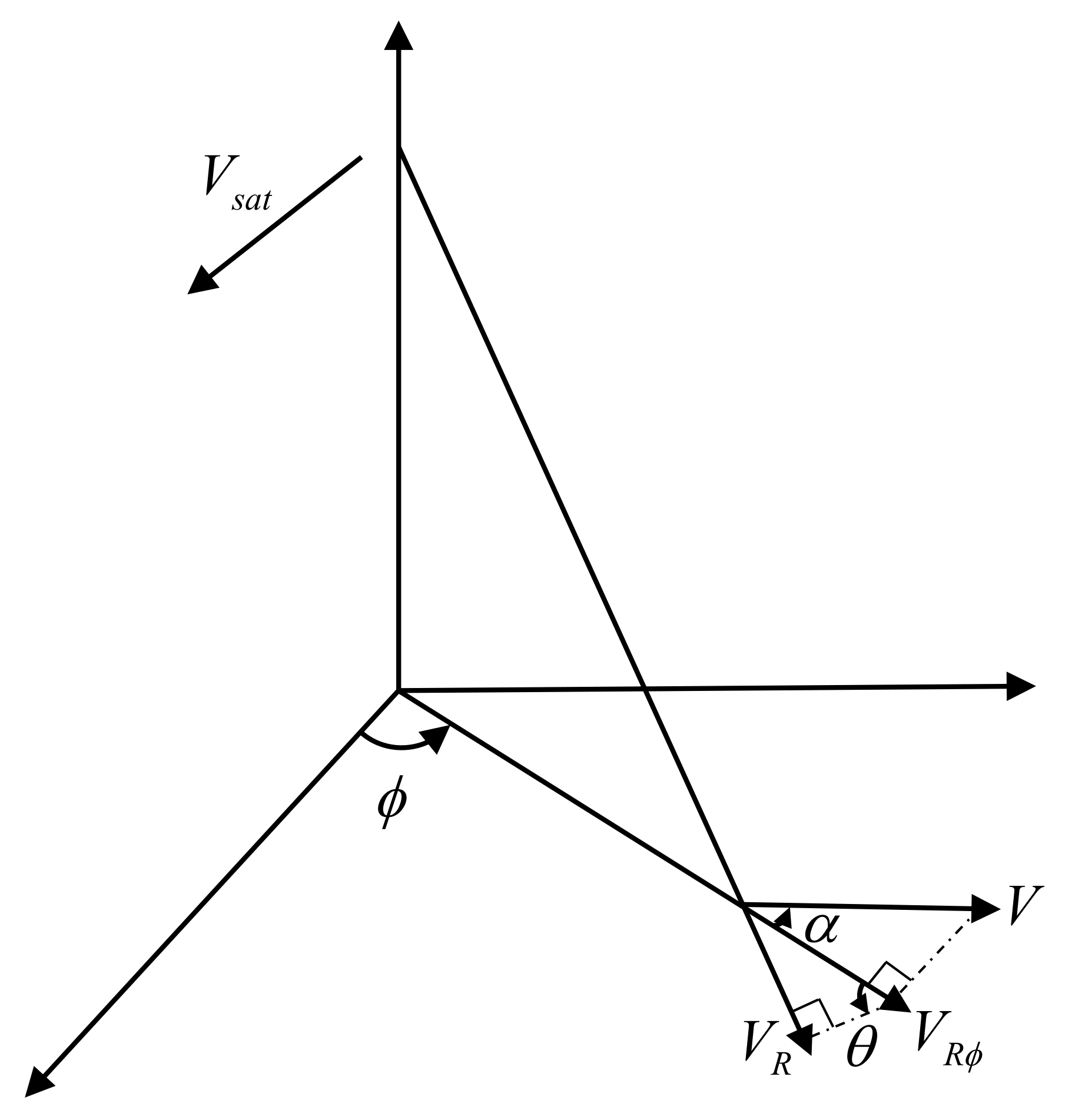
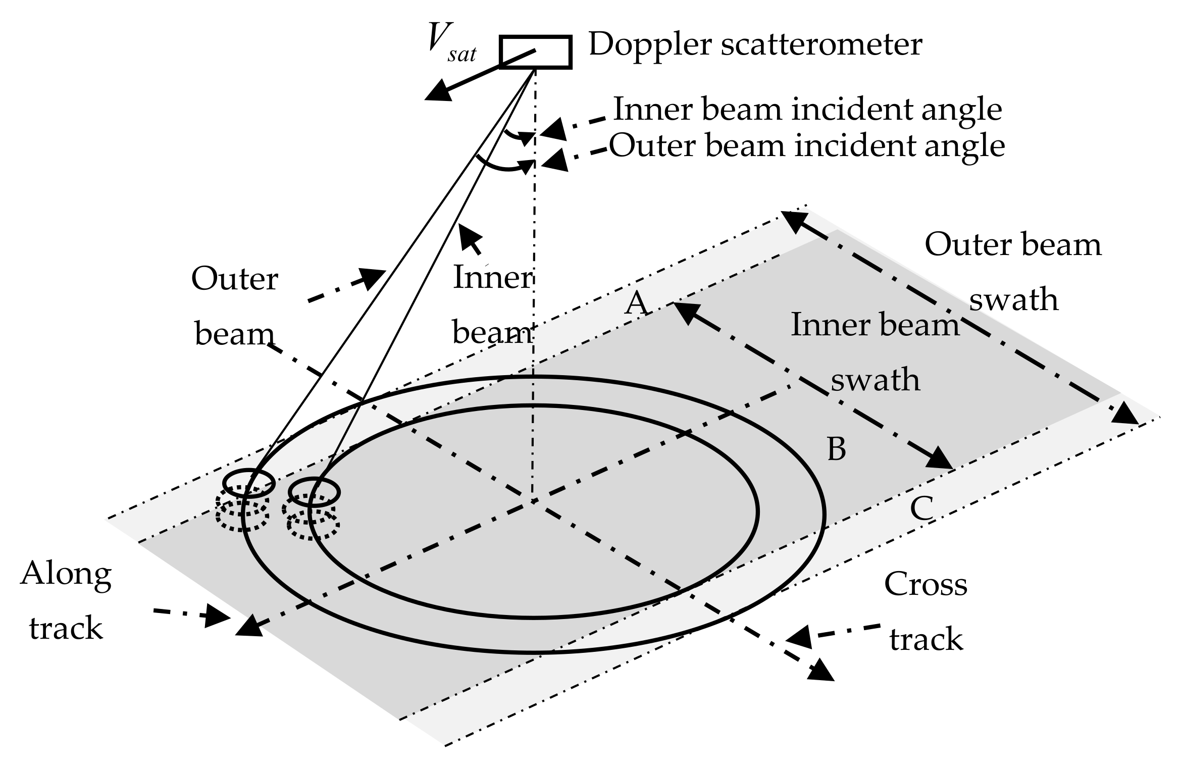
2. The Principle of Ocean Current Velocity Measurement Using Doppler Scatterometry

Doppler scatterometry transmits two signals separately within a sufficiently short time interval to observe the same sea surface area, and the radial motion of ocean currents will cause a phase change in the backscattered signal. The interference phase difference can be obtained from two corresponding echo signals and used to estimate the current radial speed [23].

The geometric configuration for ocean current observation with Doppler scatterometry is shown in Figure 1. In the three-dimensional X-Y-Z coordinate system, S and Q represent the positions of the Doppler scatterometer and observation point, respectively. $V_{sat}$ denotes the satellite speed, $V$, $V_R$, and $V_{R\varphi }$ represent the current vector velocity magnitude, radial component, and the component along the observation azimuth $\varphi$ at the position Q, respectively. $\alpha$ indicates the intersection angle between the sea surface current direction and observation azimuth $\varphi$, $\theta$ is the local incident angle. According to the projection relationship, $V$, $V_R$, and $V_{R\varphi }$ are related by

$$V=\frac{V_{R\varphi }}{\cos \alpha }=\frac{V_R}{\cos \alpha \sin \theta }.$$

(1)

Let us denote $\tau$ as the time interval between Doppler scatterometer’s two consecutive observations for the same location, $\lambda$ as the wavelength of the transmitted electromagnetic wave. The relationship between $V_R$ and the interference phase difference $\Delta \mathsf{\Phi }$ from two echo signals can be expressed as [24,25]

$$V_R=\frac{f_D\lambda }{2}=\frac{\Delta \mathsf{\Phi }\lambda }{4\pi \tau },$$

(2)

where $f_D$ represents the Doppler frequency shift. Based on Equation (2), the radial current speed $V_R$ along any observation azimuth can be obtained. Then the vector current velocity can be calculated using radial current speeds estimated from two or more different observation azimuths.

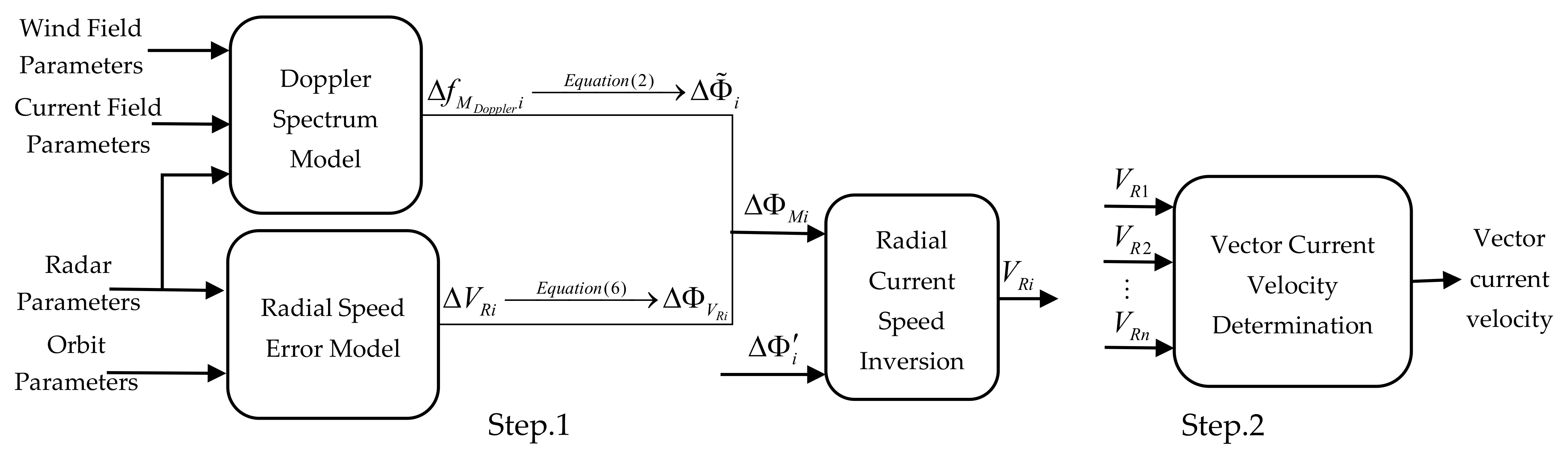
3. The Proposed Ocean Current Velocity Determination Method

Doppler scatterometry is a newly proposed scatterometer system and is currently in its pre-research stage [20], no such real radar system has been developed. Therefore, the research on Doppler scatterometry is based on simulation data.

The ocean current velocity inversion procedure consists of three modules, including the data simulation module, radial current speed inversion module, and vector current velocity determination module, as shown in Figure 2.

3.1. Data Simulation Module

The data simulation module generates Doppler frequency shift data and radial speed error data first using the Doppler spectrum model and then the radial speed error model, respectively. Next, the interference phase difference data required for the radial current speed inversion module can be obtained according to Equation (2).

With sea surface wind field and current field information, radar parameters, satellite orbit parameters as input, the numerical Doppler spectrum model proposed by Romeiser and Thompson [24] is used to produce the sea-echo Doppler spectra with and without ocean current, respectively. Then, the Doppler frequency shift $\Delta f_{M_{Doppler}}$ caused by ocean current can be obtained by calculating the center frequency shift between two Doppler spectra.

Let us denote $f_{M_{Doppler}i}$ as the Doppler center frequency at the ith observation for which the observation azimuth is ${\varphi }_i$, then

$$f_{M_{Doppler}i}=F\left(M_{Doppler}\left(V_{Ri},U_{wind},{\varphi }_{wind},{\theta }_i,{\varphi }_i,p_i\right)\right),$$

(3)

where $M_{Doppler}(\cdot )$ represents the Doppler spectrum model, $F(\cdot )$ represents the centroid calculation operation. $V_{Ri}$ is the radial speed, $U_{wind}$ and ${\varphi }_{wind}$ represent the wind speed and wind direction at 10 m above the sea surface. $p_i$ denotes either HH or VV polarization. ${\theta }_i$ represents the electromagnetic wave local incident angle.

The sea-echo Doppler spectra without current $f_{M_{Doppler}i}^0$ can be calculated by setting $V_{Ri} = 0$, and the Doppler center frequency shift $\Delta f_{M_{Doppler}i}$ can be obtained as

$$\Delta f_{M_{Doppler}i}=f_{M_{Doppler}i}-f_{M_{Doppler}i}^0.$$

(4)

Then the interference phase difference $\Delta {\tilde{\mathsf{\Phi }}}_i$ at the ith observation can be calculated using Equation (2) by substituting the Doppler frequency shift $\Delta f_{M_{Doppler}i}$ for $f_D$.

In a real measurement scenario, due to the influence of the radar system parameters and observation geometry measurement error $\Delta V_m$, the platform velocity measurement error $\Delta V_P$, and the Doppler spectrum model error $\Delta V_d$ [20], the estimated radial current speed inevitably has errors. The radial speed error model is used to simulate the radial speed error $\Delta V_R$ caused by the aforementioned factors. Assume $\Delta V_m$, $\Delta V_P$, and $\Delta V_d$ are normally distributed and independent of each other, the radial speed error $\Delta V_R$ can be expressed as [20]

$$\Delta V_R=\sqrt{\Delta V_m{}^2+\Delta V_p{}^2+\Delta V_d{}^2}.$$

(5)

The measurement error of the interference phase difference caused by the radial speed error $\Delta V_R{}_i$ can be expressed as

$$\Delta {\mathsf{\Phi }}_{V_{Ri}}=2\pi \frac{2\Delta V_{Ri}}{\lambda }\tau .$$

(6)

Then the interference phase difference $\Delta {\mathsf{\Phi }}_{Mi}$ from two radar echoes measured by Doppler scatterometer can be expressed as

$$\Delta {\mathsf{\Phi }}_{Mi}=\Delta {\tilde{\mathsf{\Phi }}}_i+\Delta {\mathsf{\Phi }}_{V_{Ri}},$$

(7)

where $\Delta {\tilde{\mathsf{\Phi }}}_i$ denotes the ideal interference phase difference.

The data simulation procedure is summarized in Algorithm 1.

Algorithm 1 Data simulation for Doppler scatterometer.

1: Input: The local incident angles ${\theta }_1$ and ${\theta }_2$, the observation azimuths ${\varphi }_1$, ${\varphi }_2$,

2: and ${\varphi }_3$, polarization mode $p_1$ and $p_2$, wind field parameters $U_{wind}$ and ${\varphi }_{wind}$, the

3: current field parameters $V_{current}$ and ${\varphi }_{current}$.

4: Output: The simulated interference phase difference measurements $\Delta {\mathsf{\Phi }}_{M1}$,

5: $\Delta {\mathsf{\Phi }}_{M2}$, and $\Delta {\mathsf{\Phi }}_{M3}$.

6: ① For an observation position on the sea surface, radial current speeds $V_{R1}$, $V_{R2}$,

7: and $V_{R3}$ in three different observation azimuths ${\varphi }_1$$, {\varphi }_2$, and ${\varphi }_3$ are calculated

8: using Equation (1) according to the given ocean current velocity.

9: ② The echo-Doppler spectra along three observation azimuths are calculated using

10: the Doppler spectrum model [24] with ${\varphi }_1$$, {\varphi }_2$, ${\varphi }_3$, $U_{wind}$, ${\varphi }_{wind}$, $V_{R1}$$, V_{R2}$$, V_{R3}$,

11: ${\theta }_1$, ${\theta }_2$, $p_1$ and $p_2$ as input parameters. The corresponding Doppler spectra for

12: $V_{R1}=0$$, V_{R2}=0$ and $V_{R3}=0$ can also be obtained.

13: ③ Based on the obtained Doppler spectra, the Doppler center frequencies can be

14: calculated using Equation (3). Then the Doppler frequency shifts $\Delta f_{M_{Doppler}1}$,

15: $\Delta f_{M_{Doppler}2}$ and $\Delta f_{M_{Doppler}3}$ can be obtained based on Equation (4).

16: ④ The ideal echo interference phase differences $\Delta {\tilde{\mathsf{\Phi }}}_1$$, \Delta {\tilde{\mathsf{\Phi }}}_2$$\mathrm{and} \Delta {\tilde{\mathsf{\Phi }}}_3$ for obser-

17: vation azimuths ${\varphi }_1$$, {\varphi }_2$ and ${\varphi }_3$ can be respectively calculated using Equation (2)

18: with the obtained $\Delta f_{M_{Doppler}1}$, $\Delta f_{M_{Doppler}2}$ and $\Delta f_{M_{Doppler}3}$.

19: ⑤ The radial current speed error model is used to generate the radial current speed

20: error $\Delta V_{R1}$$, \Delta V_{R2}$ and $\Delta V_{R3}$ in observation azimuths ${\varphi }_1$$, {\varphi }_2$ and ${\varphi }_3$. Then

21: Equation (6) is applied to obtain the interference phase difference $\Delta {\mathsf{\Phi }}_{V_{R1}}$$, \Delta {\mathsf{\Phi }}_{V_{R2}}$

22: and $\Delta {\mathsf{\Phi }}_{V_{R3}}$ caused by $\Delta V_{R1}$$, \Delta V_{R2}$ and $\Delta V_{R3}$.

23: ⑥ The simulated interference phase difference measurements $\Delta {\mathsf{\Phi }}_{M1}$$, \Delta {\mathsf{\Phi }}_{M2}$ and

24: $\Delta {\mathsf{\Phi }}_{M3}$ are calculated using Equation (7) with the obtained $\Delta {\tilde{\mathsf{\Phi }}}_1$ and $\Delta {\mathsf{\Phi }}_{V_{R1}}$$, \Delta {\tilde{\mathsf{\Phi }}}_2$

25: and $\Delta {\mathsf{\Phi }}_{V_{R2}}$$, \Delta {\tilde{\mathsf{\Phi }}}_3$ and $\Delta {\mathsf{\Phi }}_{V_{R3}}$.

3.2. Radial Current Speed Inversion Module

The function of the radial current speed inversion module is to use the interference phase difference matching method to estimate the radial current speed. Suppose that the radial current speed at a certain position on the sea surface is $V_{Ri}^{\prime }$ for the ith observation, then the corresponding interference phase difference can be calculated as $\Delta {\mathsf{\Phi }}_i^{\prime }=2\pi \frac{2V_{Ri}^{\prime }}{\lambda }\tau$. Let

$$\Delta {\mathsf{\Phi }}_i^{\prime }=\Delta {\mathsf{\Phi }}_{Mi},$$

(8)

then the value of $V_{Ri}^{\prime }$ that satisfies the above equation be the determined radial current speed. In this way, the radial current speeds under different observation azimuths can be estimated from measured interference phase difference $\Delta {\mathsf{\Phi }}_{Mi}$ in different observation azimuths.

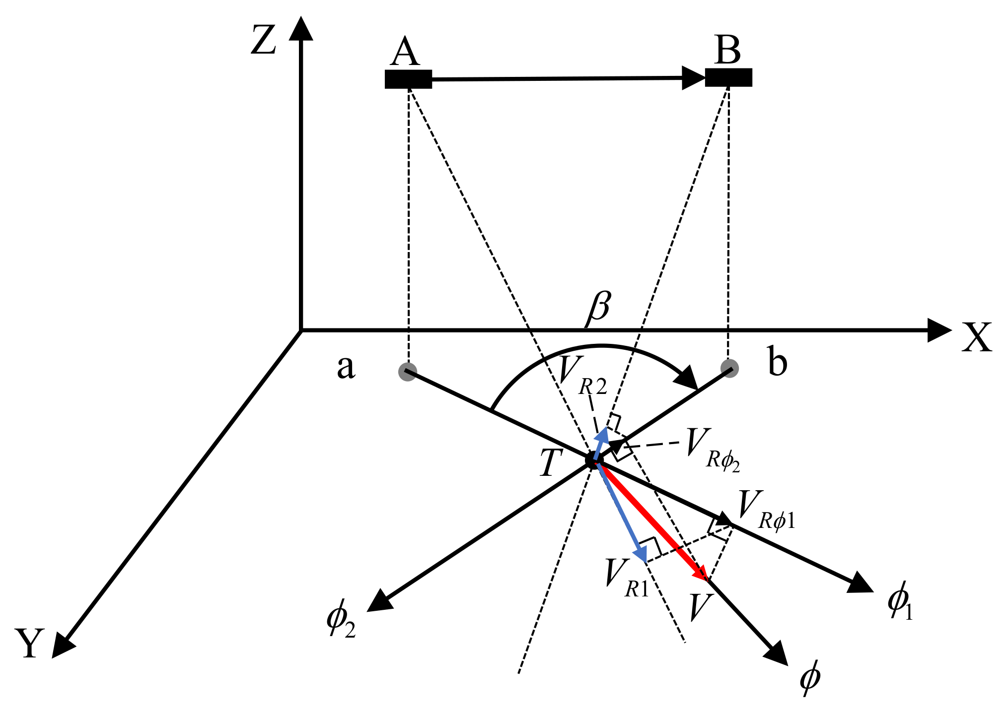
3.3. Vector Current Velocity Determination Module

Doppler scatterometer utilizes a rotating antenna system to scan the sea surface using an inner beam with HH polarization and an outer beam with VV polarization, which enables it to observe the same patch of the sea surface from up to four different observation azimuths (two from the inner beam and the other two from the outer beam) [19], as shown in Figure 3. It can be seen from Figure 3 that different scanning swaths can be obtained with inner and outer beams, and the scanning swath of the inner beam is covered by that of the outer beam. Due to antenna rotation, a sea surface patch may be observed twice by the inner beam or outer beam. Therefore, for the sea surface patch located within the scanning swath of the inner beam (region B in Figure 3), it may be observed with up to four different observation azimuths. While for the sea surface patch located in the non-overlapping regions of two scanning swaths (regions A and C in Figure 3), it may only be observed by two different observation azimuths at most. The vector current velocity determination module generates vector current velocities using the radial current components estimated from two or more different observation azimuths. If an area of the sea surface is covered by the footprints of only two different observation azimuths, the corresponding sea surface vector current velocity is determined using the estimated radial speeds along these two observation azimuths. If it is covered by the footprints of three or more different observation azimuths, the corresponding vector current velocity can be determined using the radial current speeds of two optimal observation azimuths chosen by an optimal observation azimuth selection method. In this method, a preliminary estimate of the current direction at the observation position is obtained based on vector summation of two radial current components estimated from two arbitrarily selected different observation azimuths. Then, the two observation azimuths that have the smallest differences with the preliminarily estimated current direction are selected as the optimal observation azimuths. Finally, the radial current speeds obtained using Equations (8) and (2) from the two optimally selected observation azimuths are used to produce the sea surface vector current velocity via a vector current determination method.

3.3.1. Proposed Vector Current Velocity Determination Method

The vector current velocity is determined using two radial current components. In [20,26], the parallelogram method is used for vector current velocity calculation. However, since the radial current speeds along different observation azimuths are the projected components of true current velocity, they are not independent of each other. The parallelogram method for vector determination is not applicable except when the intersection angle $\beta$ between two observation azimuths is 90°.

As shown in Figure 4, for a specific position T at the sea surface, the vector current velocity magnitude and direction are denoted as $V$ and $\varphi$, respectively. Suppose the Doppler scatterometer moves from position $A$ towards position $B$, $a$ and $b$ are the corresponding sub-satellite points. At position $A$ where the corresponding observation azimuth is ${\varphi }_1$ and the local incident angle is ${\theta }_1$, it obtains a radial current speed $V_{R1}$, at position $B$ the observation azimuth is ${\varphi }_2$, the local incident angle is ${\theta }_2$, and the observed radial current speed is $V_{R2}$. The velocity components along the observation azimuths ${\varphi }_1$ and ${\varphi }_2$ at the position T are denoted as $V_{R{\varphi }_1}$ and $V_{R{\varphi }_2}$, respectively. Thus, the intersection angle between two observation azimuths is $\beta = {\varphi }_2 - {\varphi }_1$.

It can be noticed that when the vector current velocity magnitude $V$, direction $\varphi$, and observation azimuths ${\varphi }_1$ and ${\varphi }_2$ are known, the relationship between the radial current speeds $V_{R1}$, $V_{R2}$ and the vector current velocity is also determined. Based on this consideration, a new vector current determination method utilizing the projection relationship is proposed.

It should be pointed out that ${\theta }_1$ and ${\theta }_2$ each could be the local incident angle of either the inner beam or the outer beam. According to Equation (1), the relationship between $V_{R1}$, $V_{R2}$, and $V$ can be formularized as

$$V_{R1}=V_{R{\varphi }_1}\sin {\theta }_1 =V\cos \left(\varphi -{\varphi }_1\right)\sin {\theta }_1,$$

(9)

$$V_{R2}=V_{R{\varphi }_2}\sin {\theta }_2 =V\cos \left(\varphi -{\varphi }_2\right)\sin {\theta }_2.$$

(10)

Dividing Equation (9) by Equation (10) leads to

$$\frac{V_{R1}}{V_{R2}}=\frac{V\cos \left(\varphi -{\varphi }_1\right)\sin {\theta }_1}{V\cos \left(\varphi -{\varphi }_2\right)\sin {\theta }_2}=\frac{\sin {\theta }_1\left(\cos \varphi \cos {\varphi }_1+\sin \varphi \sin {\varphi }_1\right)}{\sin {\theta }_2\left(\cos \varphi \cos {\varphi }_2+\sin \varphi \sin {\varphi }_2\right)},$$

(11)

which can be reduced to

$$\cos \varphi \left(V_{R1}\cos {\varphi }_2\sin {\theta }_2-V_{R2}\cos {\varphi }_1\sin {\theta }_1\right)=\sin \varphi \left(V_{R2}\sin {\varphi }_1\sin {\theta }_1-V_{R1}\sin {\varphi }_2\sin {\theta }_2\right).$$

(12)

Dividing both sides of Equation (12) by $\cos \varphi$, the tangent function of the ocean current direction can be obtained as

$$\tan \varphi =\frac{V_{R1}\cos {\varphi }_2\sin {\theta }_2-V_{R2}\cos {\varphi }_1\sin {\theta }_1}{V_{R2}\sin {\varphi }_1\sin {\theta }_1-V_{R1}\sin {\varphi }_2\sin {\theta }_2}$$

(13)

Therefore, the current velocity direction can be derived as

$$\varphi =\arctan \left(\frac{V_{R1}\cos {\varphi }_2\sin {\theta }_2-V_{R2}\cos {\varphi }_1\sin {\theta }_1}{V_{R2}\sin {\varphi }_1\sin {\theta }_1-V_{R1}\sin {\varphi }_2\sin {\theta }_2}\right).$$

(14)

Then, the magnitude of the vector current velocity can be calculated by

$$V=\frac{V_{R1}}{\cos \left(\varphi -{\varphi }_1\right)\sin {\theta }_1}.$$

(15)

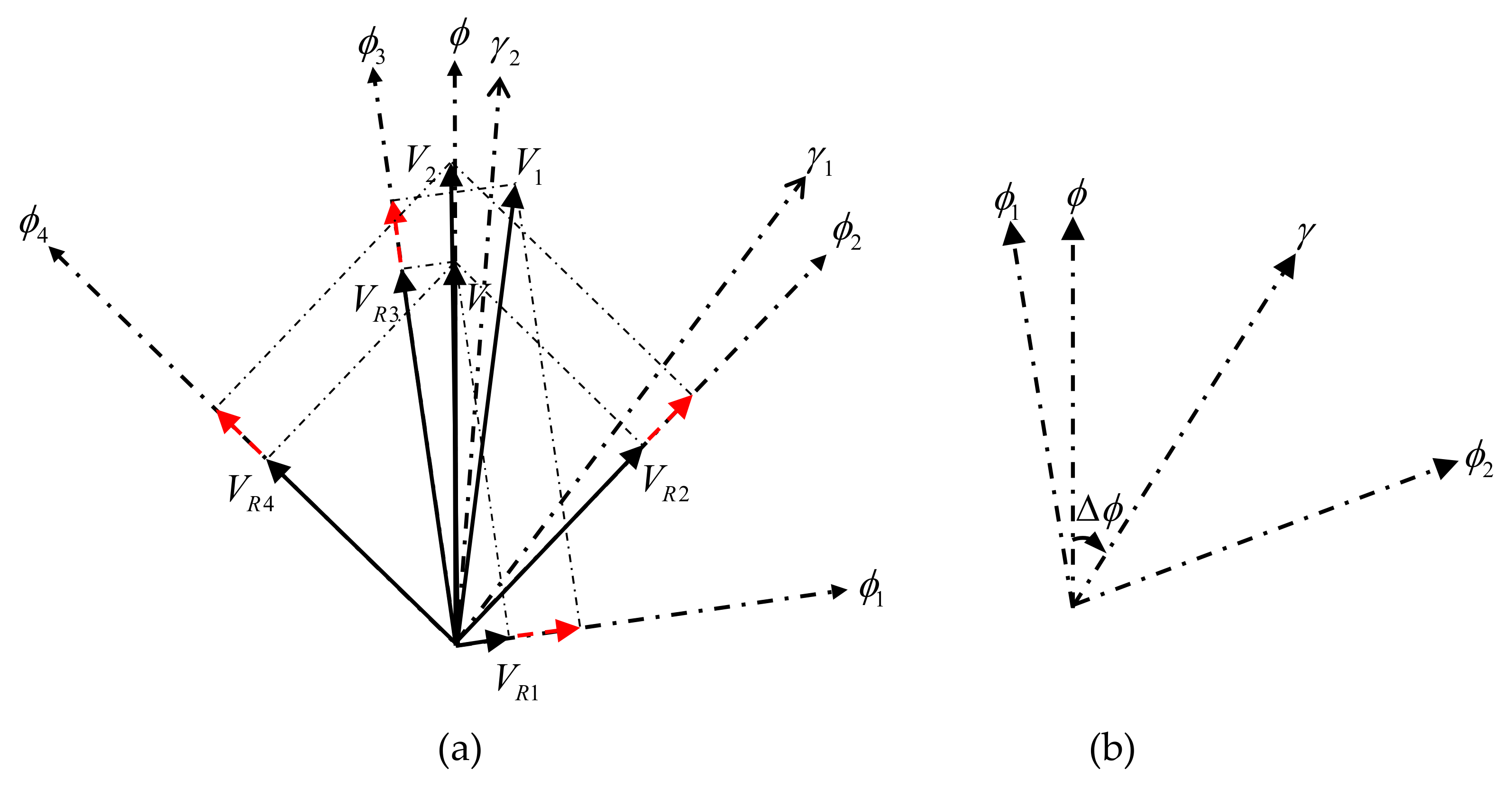
3.3.2. A Method for Optimal Observation Azimuth Selection

Doppler scatterometry can realize multi-azimuth observation of a same sea surface position using a rotating scanning antenna system, the vector current velocity at the observation position can be calculated using the radial current speeds obtained from different observation azimuths. As shown in Figure 5, at a specific observation position $O$, the magnitude and direction of the true current velocity $\overrightarrow{V}$ are assumed to be $V$ and $\varphi$, respectively. As mentioned in [19], Doppler scatterometry can observe a position from up to four different observation azimuths from both inner and outer beams—say ${\varphi }_1$, ${\varphi }_2$, ${\varphi }_3$, and ${\varphi }_4$. The projected components of $V$ on these four observation azimuths are $V_{R1}$, $V_{R2}$, $V_{R3}$, and $V_{R4}$, respectively. ${\gamma }_1$ and ${\gamma }_2$ represent the bisector directions of ${\varphi }_1$ and ${\varphi }_3$, ${\varphi }_2$, and ${\varphi }_4$, respectively. $\Delta \varphi$ is the intersection angle between the current direction $\varphi$ and the positive or negative direction of $\gamma$, which is the bisector of two observation azimuths (see Figure 5b). Although there are slight differences in radial current speed errors along different observation azimuths due to different local incident angles of the inner beam and outer beam, a constant radial current speed error $\Delta V_R$ is assumed and represented by dotted lines with red arrows for simplicity, as shown in Figure 5a. It should be pointed out that, in Section 4 (Experimental Results), the radial speed error data were generated according to the radial speed error model in Equation (5) to consider the error variation due to different observation azimuths and incident angles. In Figure 5a, ${\overrightarrow{V}}_1$ is derived from $V_{R1}$, $V_{R3}$, and $\Delta V_R$; while ${\overrightarrow{V}}_2$ is derived with $V_{R2}$, $V_{R4}$, and $\Delta V_R$. It can be noticed that a vector current velocity can be determined by any two radial current components. However, due to the error introduced in radial current speed estimation, the derived results may be different when different combinations of radial components are used. Here, the influence of a constant radial speed error $\Delta V_R$ from different observation azimuths on the final vector current velocity result will be analyzed.

It can be seen from Figure 5a that two derived results ${\overrightarrow{V}}_1$ and ${\overrightarrow{V}}_2$ are of similar velocity magnitudes, but the direction of ${\overrightarrow{V}}_2$ is almost the same as that of $\overrightarrow{V}$, thus the velocity direction estimation error of ${\overrightarrow{V}}_2$ is smaller than that of ${\overrightarrow{V}}_1$. It can be concluded that the inversion accuracy of vector current velocity is different using different radial current component combinations. The smaller the intersection angle between the true current direction and the positive or negative direction of the bisector of two observation azimuths is, the higher the accuracy of current inversion is. Therefore, it is necessary to select the optimal observation azimuths for vector current velocity calculation to reduce the influence of the radial speed error.

Based on the above analysis, an optimal observation azimuth selection method is proposed and described as follows. Assume a Doppler scatterometer observes one sea surface patch from three different azimuths—${\varphi }_1$, ${\varphi }_2$, and ${\varphi }_3$, respectively—then there are three possible combinations for vector current velocity determination—i.e., the radial current components in ${\varphi }_1$ and ${\varphi }_2$, ${\varphi }_1$ and ${\varphi }_3$, ${\varphi }_2$ and ${\varphi }_3$.

Firstly, two radial current components are arbitrarily selected and used to obtain a preliminary estimation ${\varphi }_p$ of the current direction. Then the intersection angle $\Delta \varphi$ between ${\varphi }_p$ and the bisector direction of the observation azimuths of each combination can be calculated as

$$\begin{gathered} \Delta {\varphi }_1=\min \left(\left|\frac{1}{2}\left({\varphi }_1+{\varphi }_2\right)-{\varphi }_p\right|,\left|\frac{1}{2}\left({\varphi }_1+{\varphi }_2\right)+\pi -{\varphi }_p\right|\right), \\ \Delta {\varphi }_2=\min \left(\left|\frac{1}{2}\left({\varphi }_2+{\varphi }_3\right)-{\varphi }_p\right|,\left|\frac{1}{2}\left({\varphi }_2+{\varphi }_3\right)+\pi -{\varphi }_p\right|\right), \\ \Delta {\varphi }_3=\min \left(\left|\frac{1}{2}\left({\varphi }_1+{\varphi }_3\right)-{\varphi }_p\right|,\left|\frac{1}{2}\left({\varphi }_1+{\varphi }_3\right)+\pi -{\varphi }_p\right|\right). \end{gathered}$$

(16)

Then the optimal observation azimuth combination $\left({\varphi }_{Opt1},{\varphi }_{Opt2}\right)$ is selected as that produces the minimum intersection angle, i.e.,

$$\left({\varphi }_{Opt1},{\varphi }_{Opt2}\right)=\arg \min \left(\Delta {\varphi }_1,\Delta {\varphi }_2,\Delta {\varphi }_3\right).$$

(17)

Next, the radial current components obtained from observation azimuths ${\varphi }_{Opt1}$ and ${\varphi }_{Opt2}$ are selected and used to derive the final vector current velocity using the proposed vector current velocity determination method described in Section 3.3.1.

The proposed vector current velocity determination method for Doppler scatterometry is summarized in Algorithm 2.

Algorithm 2 Vector current velocity estimation based on optimally selected observation azimuths.

1: Input: The observation azimuths ${\varphi }_1$$, {\varphi }_2$, and ${\varphi }_3$, the measured interference phase

2: difference $\Delta {\mathsf{\Phi }}_{M1}$$, \Delta {\mathsf{\Phi }}_{M2}$, and $\Delta {\mathsf{\Phi }}_{M3}$.

3: Output: The vector current velocity at an observation position.

4: ① According to $\Delta {\mathsf{\Phi }}_{M1}$$, \Delta {\mathsf{\Phi }}_{M2}$, and $\Delta {\mathsf{\Phi }}_{M3}$, the radial current speeds $V_{R1}^{\prime }$$, V_{R2}^{\prime }$, and

5: $V_{R3}^{\prime }$ in ${\varphi }_1$$, {\varphi }_2$, and ${\varphi }_3$ are estimated using the interference phase difference

6: matching method (see Equation (8)).

7: ② Any two radial current speeds from two different observation azimuths are se-

8: lected to determine a vector current velocity using Equations (13) and (14). The

9: obtained current direction ${\varphi }_p$ is used as a preliminary estimation of the current

10: direction.

11: ③ The optimal observation azimuths ${\varphi }_{Opt1}$ and ${\varphi }_{Opt2}$ are determined using

12: Equations (15) and (16) with ${\varphi }_1$$, {\varphi }_2$$, {\varphi }_3$, and ${\varphi }_p$ as input.

13: ④ The final vector current velocity is obtained using Equations (13) and (14) with

14: radial current speeds obtained from observation azimuths ${\varphi }_{Opt1}$ and ${\varphi }_{Opt2}$.

4. Experimental Results

In order to verify the effectiveness of the proposed method, current velocity estimation experiments were conducted with simulated Doppler scatterometer data, as well as OSCAR data [20]. OSCAR data—including 2500 sampling points with latitudes from 10° to 50° and longitudes from −70° to −30° that were acquired on January 28, 2020 —were used as current field data.

4.1. Data Simulation Results and Analysis

The numerical Doppler spectrum model based on interferometry principle established by Romeiser and Thompson [24] and the system parameters of a Doppler scatterometer listed in

Table 2. Parameters of the Doppler scatterometer for data simulation.

Parameters	Specification
Satellite Velocity	7373 m/s
Orbit Altitude	963 km
Observation Azimuth	10°, 30°, and 170°
Local Incident Angle	${41}^{°}(\mathrm{H}\mathrm{H})/{48}^{°}(\mathrm{V}\mathrm{V})$
Antenna Incident Angle	${35}^{°}(\mathrm{H}\mathrm{H})/{41}^{°}(\mathrm{V}\mathrm{V})$
Antenna Gain	48 dB
Rotation Rate	18 rpm
Carrier Frequency	13.5 GHz
PRF	12 kHz
Pulse Bandwidth	5 MHz

were used for data simulation.

In order to verify the correctness and applicability of the Doppler spectrum model, the Doppler spectra for different radial current speeds ranging from 0.2 m/s to 1.4 m/s with a step size of 0.2 m/s are simulated, and the results were compared with those generated without current to obtain the Doppler center frequency shifts. Meanwhile, the Doppler frequency shifts are also calculated directly using $f_D=\frac{2V_R}{\lambda }=\frac{2V\cos \alpha \sin \theta }{\lambda }$ according to Equation (2). The corresponding results are shown in Figure 6.

It can be seen from Figure 6a that the peak position of the Doppler spectra moves right along the Doppler frequency axis with increasing radial current speed. It verifies the fact that the larger the radial current speed is, the larger the Doppler frequency shift is. Figure 6b shows the variation trend of Doppler frequency shift with increasing radial current speed. It can be noticed that the Doppler frequency shifts calculated from Doppler center frequency difference agree well with those calculated using Equation (2). The results verify that the Doppler spectrum model is appropriate.

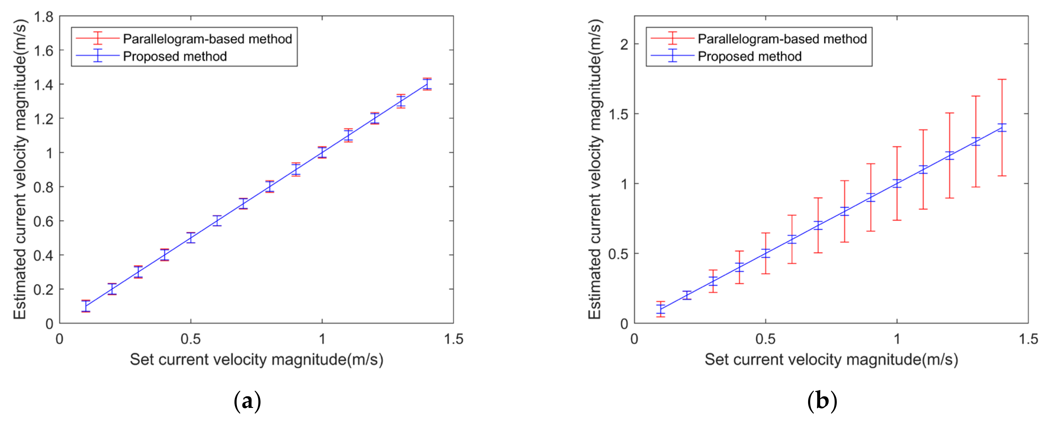
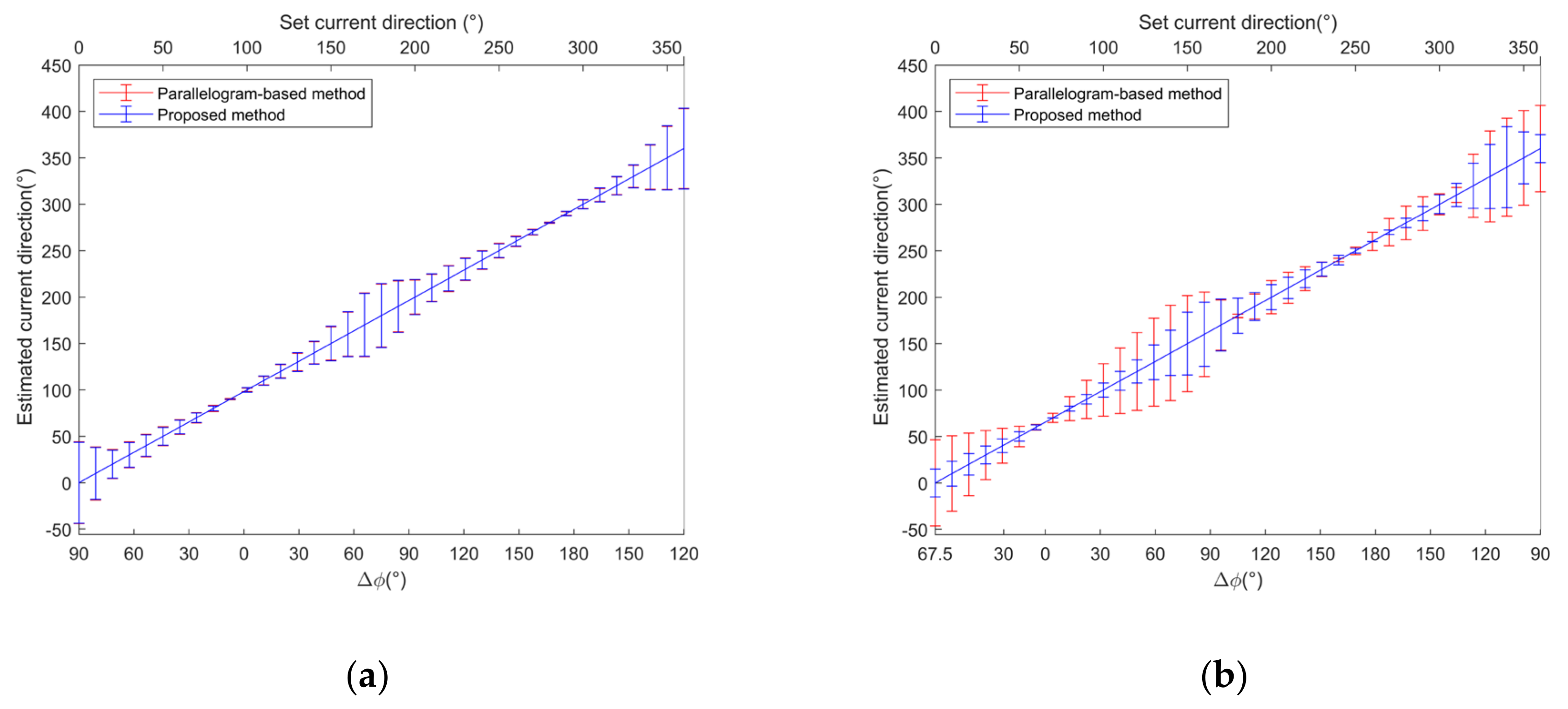
4.2. Verification of the Proposed Vector Current Velocity Determination Method

In order to test the applicability and effectiveness of the proposed vector current velocity determination method, both it and the parallelogram-based method were applied to two observation azimuth combinations—45° and 90°, 45° and 135° (refer to ASCAT) [19]—to estimate the current velocity magnitude and direction, respectively.

Firstly, to evaluate the accuracy of current velocity magnitude inversion, the current direction was fixed to 0°, the current velocity magnitude varied from 0.1 m/s to 1.4 m/s with a step size of 0.1 m/s. The estimated current velocity magnitudes using the proposed method and parallelogram-based method are illustrated in Figure 7a (for $\beta ={90}^{\circ }$) and Figure 7b (for $\beta \ne {90}^{\circ }$), respectively.

It can be seen from Figure 7a that for $\beta ={90}^{\circ }$, the estimation errors of current velocity magnitude are almost the same for two methods and the estimated velocity magnitude agrees with the input value. Both methods can produce good estimation results, and the estimation errors mainly come from the radial speed errors. However, the results in Figure 7b demonstrate that, for $\beta \ne {90}^{\circ }$, the current velocity magnitude estimation error of the parallelogram-based method is larger with a maximum of 0.34 m/s and increases with the increasing current velocity. However, the proposed method achieves stable estimation results with small estimation errors of less than 0.06 m/s.

Secondly, in order to assess the performance of current direction estimation, the current velocity magnitude was set to 0.1 m/s, but the current direction varied from 0° to 360° with a step size of 10°. The estimated current velocity directions using the proposed method and parallelogram-based method are illustrated in Figure 8a (for $\beta ={90}^{\circ }$) and Figure 8b (for $\beta \ne {90}^{\circ }$), respectively.

It can be seen from Figure 8 that for $\beta ={90}^{\circ }$, the current velocity direction estimation errors of two methods are almost same, but for $\beta \ne {90}^{\circ }$ the overall current direction estimation error of the proposed method is smaller than that of the parallelogram-based method with a reduction from 5.7° to 1.2°. Moreover, it can be noticed that the current direction inversion error varies with current directions. When the intersection angle $\Delta \varphi$ between the current direction and positive or negative direction of the bisector of two observation azimuths falls in $\left[0^{\circ }{ 90}^{\circ }\right]$, the current direction inversion error increases with increasing $\Delta \varphi$. While $\Delta \varphi \in \left[{90}^{\circ }{ 180}^{\circ }\right]$, the current direction inversion error decreases with increasing $\Delta \varphi$, which is consistent with the conclusion in Section 3. The results prove that the intersection angle $\Delta \varphi$ affects the accuracy of current direction inversion. The smaller the intersection angle is, the higher the accuracy of current direction inversion is.

The results in Figure 7 and Figure 8 show that the proposed vector current velocity determination method has general applicability and produces better vector current velocity estimations.

It is worth noting that the current velocity magnitude can be well estimated using the proposed vector current velocity determination method. However, the maximum error of the estimated current direction of the proposed method reaches 40°, which is not acceptable in real application scenarios. Since it has been proven that the intersection angle $\Delta \varphi$ has significant impact on the inversion accuracy of current direction, it is necessary to optimally select the observation azimuths to further improve the current inversion accuracy.

To verify the effectiveness of the proposed optimal observation azimuth selection method in improving the accuracy of current inversion, a simulation case study based on current velocity with a magnitude of 0.1 m/s and a direction of 30° is used for evaluation. The current inversion results for three observation azimuth combinations of 45° and 90°, 90° and 135°, 45° and 135° (refer to the parameters of ASCAT) were generated. The estimated vector current velocities are shown in Figure 9 with arrows indicating the magnitude and direction of current velocities, and the direction is referenced to the due North. The true current velocity and the derived results with observation azimuth combinations of 45° and 90°, 90° and 135°, 45° and 135° are depicted in red, blue, black, and green arrows, respectively.

It can be seen from Figure 9 that the accuracy of current velocity inversion for different observation azimuth combinations is different. For the observation azimuth combinations of 45° and 90°, 90° and 135°, 45° and 135°, the intersection angles $\Delta \varphi$ between their bisector directions and true current direction are 67.5°, 112.5°, and 90°, respectively, and the estimated current directions are 32.6°, 48.6°, and 47.8°, respectively. $\Delta \varphi$ of the observation azimuth combination of 45° and 90° is the smallest, thus this pair of observation azimuths achieves the best estimation result. It is found that the observation azimuth combination of 45° and 90° is always determined as optimal by Equation (16), and the current velocity estimation using this combination obtains the highest accuracy.

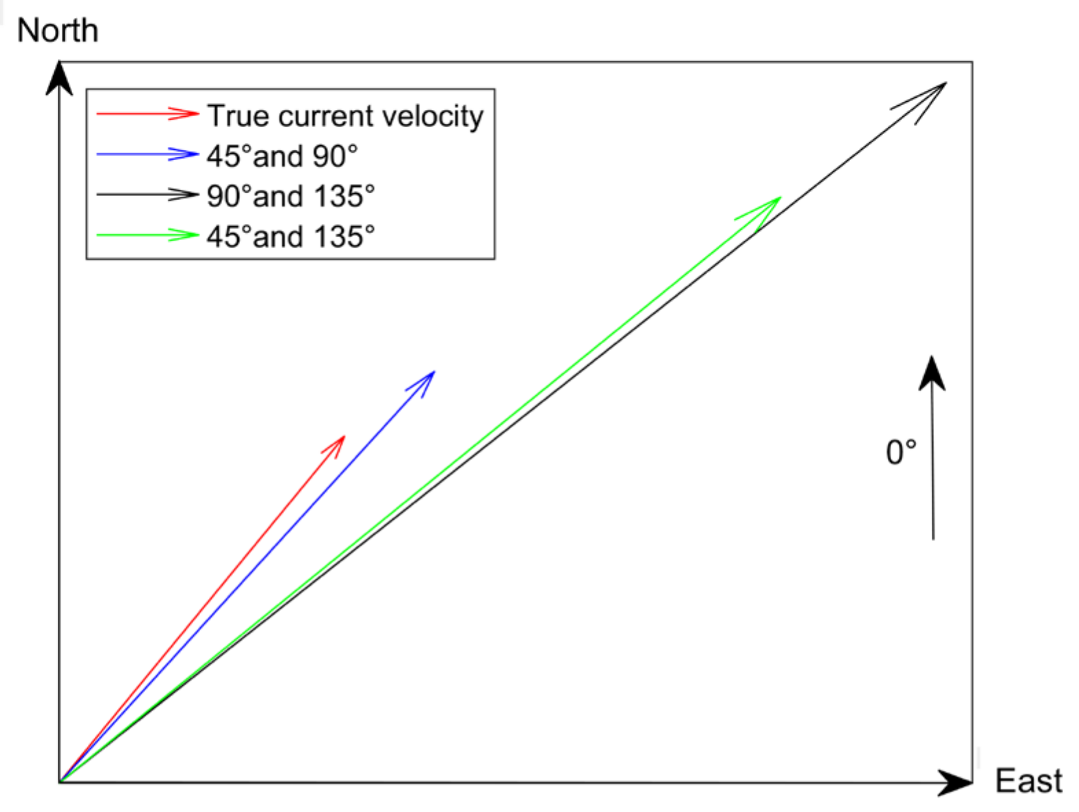
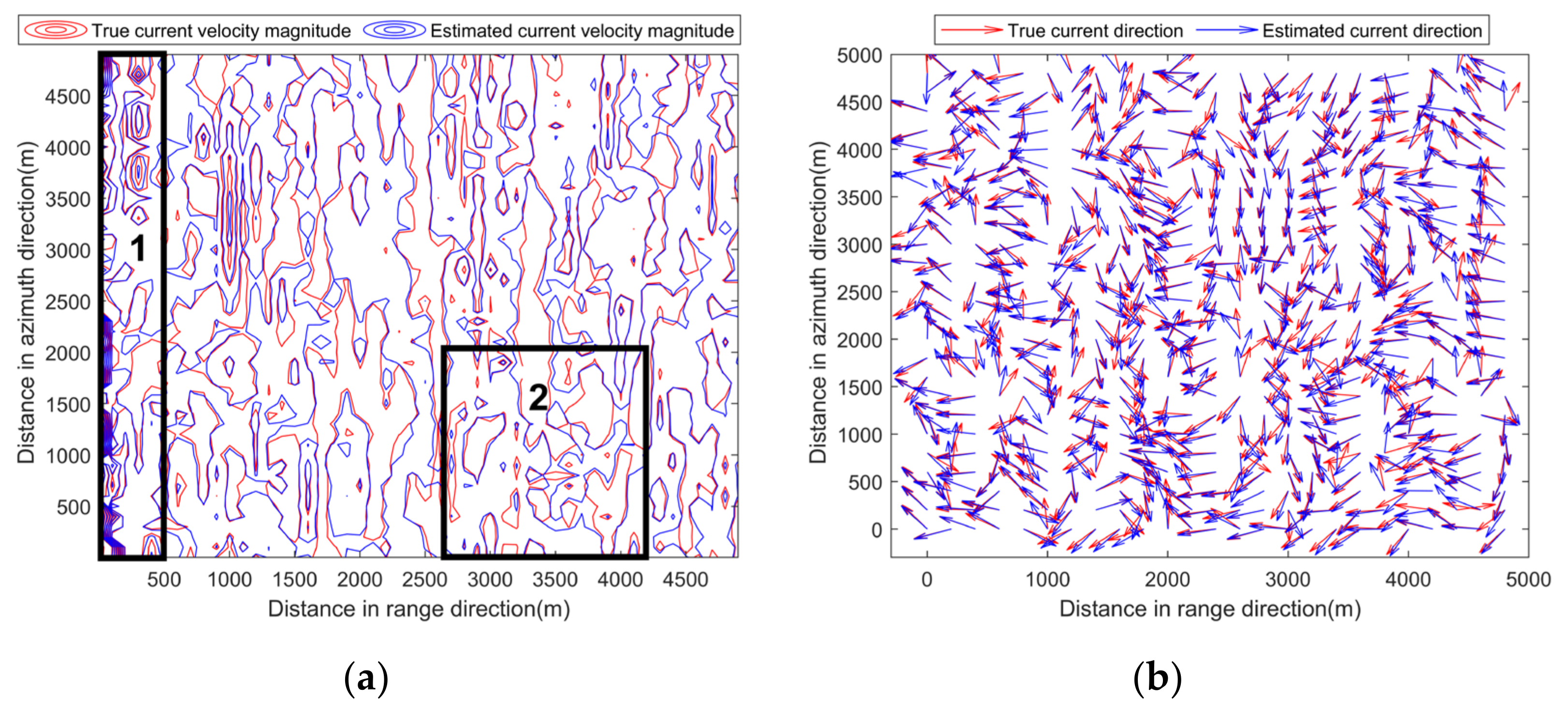
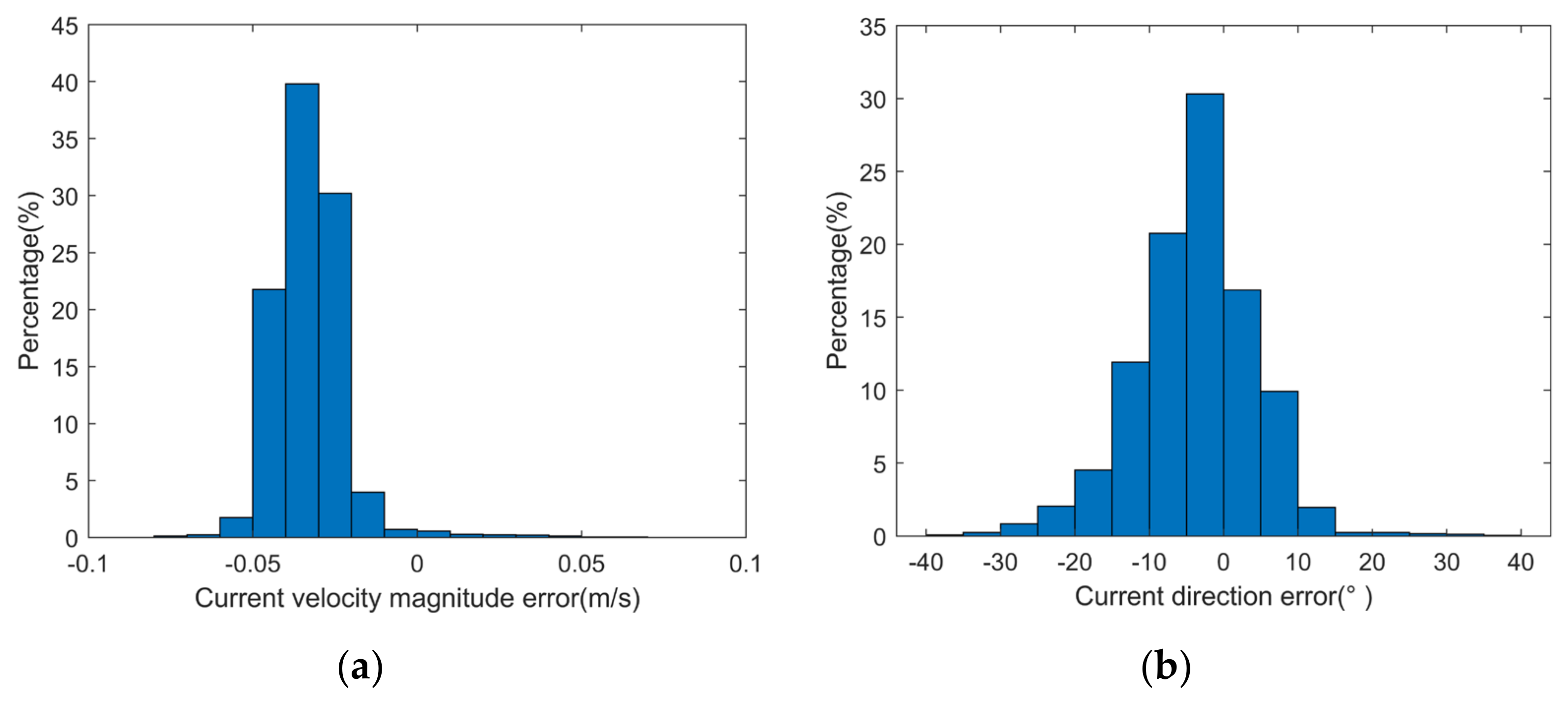
4.3. Current Velocity Inversion Results and Analysis

In order to further evaluate the performance of the proposed vector current velocity inversion method, OSCAR current data were used as test data and the radial speed error model [20] was used to generate the radial speed error data. The current velocity magnitudes vary from 0.011 m/s to 1.328 m/s, and the current directions are from 9.53° to 350.26°. $\Delta V_m$, $\Delta V_P$, and $\Delta V_d$ can be calculated based on the formulas presented in [19,20]. Referring to the parameters set in [20], for Equation (5), $\Delta V_d$ was set to 0.1 m/s, $\Delta V_m$ ranged from 0.05 m/s to 0.09 m/s, and $\Delta V_P$ ranged from 0.026 m/s to 0.033 m/s. The system parameters of the Doppler scatterometer are set according to those listed in Table 2. The observation azimuths of 10°, 30°, and 170° calculated based on the parameters set and observation geometry were used. The current velocity magnitude and direction were estimated using the proposed vector current velocity inversion method based on optimal observation azimuth selection. The estimation results are illustrated in Figure 10.

Figure 10a shows the contour map comparison between true and estimated current velocity magnitudes. The contours are dense if current velocity magnitudes are large. The degree of contour overlap between estimated and true results indicates the current inversion accuracy. The higher the overlap ratio is, the higher the inversion accuracy is. The two regions with black rectangles are selected for analysis. The contours in region 1 are dense, indicating relatively large current velocity magnitudes; while the contours in region 2 are sparse, implying small current velocity magnitudes. It can be seen from Figure 10a that the overlap degree between the estimated and true current velocity magnitude contours is higher in region 1 than that in region 2, indicating that the estimation accuracy of current velocity magnitudes is higher in region 1 than that in region 2. This is due to the influence of similar radial speed error on different current velocities. Better inversion results can be achieved for larger current velocities since the influence due to the same radial speed errors is relatively less.

Figure 10b shows the comparison between true and estimated current directions. The direction of the arrows represents the current direction. It can be seen that the correlation between the estimated and true current directions is high for most observation positions, indicating that current directions can be well estimated.

To further investigate the inversion errors of current velocity magnitude and direction, the error distributions of the estimated results are statistically calculated and shown in Figure 11.

The results in Figure 11 show that the absolute current velocity magnitude errors are less than 0.07 m/s, while 91% of the absolute current direction errors are less than 15°. The root mean square errors of current velocity magnitude and direction are 0.04 m/s and 9.05°, respectively, while the standard deviation of the estimated current velocity magnitude is 0.06 m/s. Compared with the current velocity magnitude standard deviation reported in [20], the estimation accuracy is improved by 67%.

5. Conclusions

In this paper, a vector current velocity inversion method based on optimal observation azimuth selection is proposed for Doppler scatterometry, and its effectiveness is verified with simulated and OSCAR data. The contribution of the proposed method is three-fold: (1) A radial current inversion method based on interferometric phase difference matching is proposed, which not only simplifies the current inversion process but also improves the efficiency. (2) A general vector current velocity determination method is proposed to extend its applicability. (3) The Doppler scatterometer antenna’s rotating scanning mode is well used to develop an optimal observation azimuth selection method, which further improves the current velocity inversion accuracy.

Only three observation azimuths were considered in our experiments. Actually, Doppler scatterometry can observe the same sea surface patch with up to four observation azimuths. If more observation azimuths are involved, better current velocity estimation results are expected to be achieved. It should also be pointed out that, as stated in [23], the adopted numerical Doppler spectrum model proposed by Romeiser and Thompson does not account for specular reflection and the hydrodynamic modulation of the Bragg waves induced by longer waves. Therefore, on one hand, there will be small deviations between the calculated and real Doppler frequency shifts. On the other hand, the model is limited to moderate incident angles between 30° and 60°. For incident angles outside this range, additional scattering mechanisms should be involved.

References

1. Fois, F.; Hoogeboom, P.; Chevalier, F.L.; Stoffelen, A.; Mouche, A. DopSCAT: A mission concept for simultaneous measurements of marine winds and surface currents. J. Geophys. Res. Ocean. 2015, 120, 7857–7879. [Google Scholar] [CrossRef] [Green Version]
2. Brumley, B.H.; Cabrera, R.G.; Deines, K.L.; Terray, E.A. Performance of a broad-band acoustic Doppler current profiler. IEEE J. Ocean. Eng. 1991, 16, 402–407. [Google Scholar] [CrossRef]
3. Drever, R.G.; Sanford, T.B. A free-fall electromagnetic current meter-instrumentation. In Proceedings of the Conference on Electronic Engineering in Ocean Technology, Swansea, UK, 21–24 September 1970; pp. 353–370. [Google Scholar]
4. Carter, R.W.; Anderson, I.E. Accuracy of current meter measurements. J. Hydraul. Div. 1963, 4, 105–115. [Google Scholar] [CrossRef]
5. Georges, T.M.; Harlan, J.A.; Lematta, R.A. Large-scale mapping of ocean-surface currents with dual over-the-horizon radars. Lett. Nat. 1996, 379, 434–436. [Google Scholar] [CrossRef]
6. Barrick, D. History, present status, and future directions of HF surface-wave radars in the US. In Proceedings of the International Conference on Radar, Adelaide, SA, Australia, 3–5 September 2003; pp. 652–655. [Google Scholar]
7. Emery, W.J.; Baldwin, D.G.; Matthews, D.K. Sampling the Mesoscale Ocean Surface Currents with Various Satellite Altimeter Configurations. IEEE Trans. Geosci. Remote Sens. 2004, 42, 795–803. [Google Scholar] [CrossRef]
8. Romeiser, R.; Johannessen, J.; Collard, F.; Kudryavtsev, V.; Suchandt, S. Direct surface current field imaging from space by along-track InSAR and conventional SAR. In Oceanography from Space; Springer: New York, NY, USA, 2010; pp. 73–91. [Google Scholar]
9. Chapron, B.; Collard, F.; Ardhuin, F. Direct measurements of ocean surface velocity from space: Interpretation and validation. J. Geophys. Res. Oceans. 2005, 110, C07008. [Google Scholar] [CrossRef]
10. Kim, D.; Moon, W.M.; Moller, D.; Imel, D.A. Measurements of ocean surface waves and currents using L-and C-Band along-track interferometric SAR. IEEE Trans. Geosci. Remote Sens. 2003, 41, 2821–2832. [Google Scholar]
11. Martin, A.; Gommenginger, C.P.; Yves, Q. Simultaneous ocean surface current and wind vectors retrieval with squinted SAR interferometry: Geophysical inversion and performance assessment. Remote Sens. Environ. 2018, 216, 798–808. [Google Scholar] [CrossRef] [Green Version]
12. Ali, M.M.; Bhat, G.S.; Long, D.G.; Bharadwaj, S.; Bourassa, M.A. Estimating Wind Stress at the Ocean Surface from Scatterometer Observations. IEEE Geosci. Remote Sens. Lett. 2013, 10, 1129–1132. [Google Scholar] [CrossRef] [Green Version]
13. Spencer, M.W.; Wu, C.; Long, D. Improved resolution backscatter measurements with the SeaWinds Pencil-beam scatterometer. IEEE Trans. Geosci. Remote Sens. 2000, 38, 89–104. [Google Scholar] [CrossRef] [Green Version]
14. Spencer, M.W. A Methodology for the Design of Spaceborne Pencil-Beam Scatterometer Systems. Ph.D. Thesis, Brigham Young University, Provo, UT, USA, 2001. [Google Scholar]
15. Fabry, P.; Recchia, A.; de Kloe, J.; Stoffelen, A.; Husson, R.; Collard, F.; Chapron, B.; Mouche, A.; Enjolras, V.; Johannessen, J.; et al. Feasibility Study of Sea Surface Currents Measurements with Doppler Scatterometers. In Proceedings of the Esa Living Planet Symposium, Edinburgh, UK, 9–13 September 2013. [Google Scholar]
16. Bao, Q.; Dong, X.; Zhu, D.; Lang, S.; Xu, X. The feasibility of ocean surface current measurement using pencil-beam rotating scatterometer. IEEE J. Sel. Top. Appl. Earth Obs. Remote Sens. 2015, 8, 3441–3451. [Google Scholar] [CrossRef]
17. Bao, Q.; Dong, X.; Zhu, D.; Xu, X. Ocean Surface Current Measurement Using Rotating Pencil-Beam Scatterometer. Acta Electron. Sin. 2015, 43, 1200–1204. [Google Scholar] [CrossRef]
18. Fois, F.; Hoogeboom, P.; Chevalier, F.L.; Stoffelen, A. DOPSCAT: A mission concept for a Doppler wind-scatterometer. In Proceedings of the IEEE International Geoscience and Remote Sensing Symposium (IGARSS), Milan, Italy, 26–31 July 2015; pp. 2572–2575. [Google Scholar]
19. Bao, Q. System Design and Simulation of Doppler Scatterometer—Wide Swath Ocean Surface Current Measurement. Ph.D. Thesis, Department of Electromagnetic Field and Microwave Technology, University of Chinese Academy of Sciences, Beijing, China, 2015. [Google Scholar]
20. Bao, Q.; Lin, M.; Zhang, Y.; Dong, X.; Lang, S.; Gong, P. Ocean Surface Current Inversion Method for a Doppler Scatterometer. IEEE Trans. Geosci. Remote Sens. 2017, 55, 6505–6516. [Google Scholar] [CrossRef]
21. Rodríguez, E.; Wineteer, A.; Perkovic-Martin, D.; Gál, T.; Stiles, B.W.; Niamsuwan, N.; Monje, R.R. Estimating Ocean Vector Winds and Currents Using a Ka-Band Pencil-Beam Doppler Scatterometer. Remote Sens. 2018, 10, 576. [Google Scholar] [CrossRef] [Green Version]
22. Wineteer, A.; Torres, H.S.; Rodríguez, E. On the Surface Current Measurement Capabilities of Spaceborne Doppler Scatterometry. Geophys Res. Lett. 2020, 47, e2020GL090116. [Google Scholar] [CrossRef]
23. Romeiser, R.; Thompson, D.R. Numerical study on the along-track interferometric radar imaging mechanism of oceanic surface currents. IEEE Trans. Geosci. Remote Sens. 2000, 38, 446–458. [Google Scholar] [CrossRef] [Green Version]
24. Thompson, D.R. Calculation of Microwave Doppler Spectra from the Ocean Surface with a Time-Dependent Composite Model. In Radar Scattering from Modulated Wind Waves; Komen, G.J., Oost, W.A., Eds.; Kluwer: Dordrecht, The Netherlands, 1989; pp. 27–40. [Google Scholar]
25. Thompson, D.R.; Gotwols, B.L.; Keller, W.C. A comparison of Ku-band Doppler measurements at 20° incidence with predictions from a time-dependent scattering model. J. Geophys. Res. 1991, 96, 4947–4955. [Google Scholar] [CrossRef]
26. Bao, Q. A Method of Measuring Ocean Surface Current Velocity Using Real Aperture Radar. Patent CN201510542007.0, 28 August 2015. Available online: http://d.wanfangdata.com.cn/patent/CN201510542007.0 (accessed on 10 May 2021).
Figure 1. Schematic diagram of the Doppler scatterometer observation geometry.
Remotesensing 13 04263 g001
Figure 2. Flowchart of Doppler scatterometry current velocity inversion.
Remotesensing 13 04263 g002
Figure 3. The pencil-beam rotating scanning diagram.
Remotesensing 13 04263 g003
Figure 4. Schematic diagram for vector current velocity determination.
Remotesensing 13 04263 g004
Figure 5. Schematic diagram of vector current velocity determination using different observation azimuths. (a) Illustration of vector current determination. (b) Illustration of Δ ϕ .
Remotesensing 13 04263 g005
Figure 6. Doppler spectra and Doppler center frequency shifts for different radial current speeds. (a) Doppler spectra. (b) Doppler frequency shifts.
Remotesensing 13 04263 g006
Figure 7. Error bar graphs of derived velocity magnitude using different vector determination methods. (a) β = 90 (b) β 90 .
Remotesensing 13 04263 g007
Figure 8. Error bar graphs of derived velocity direction for different vector determination methods. (a) β = 90 (b) β 90 .
Remotesensing 13 04263 g008
Figure 9. Comparison of current velocity inversion results using different observation azimuth combinations.
Remotesensing 13 04263 g009
Figure 10. Comparison of measured currents and inversion results. (a) Current velocity magnitude. (b) Current direction. Region 1 indicates an area with large current velocity magnitudes, while region 2 indicates an area with small current velocity magnitudes.
Remotesensing 13 04263 g010
Figure 11. Inversion error statistics of current velocity magnitude and direction. (a) Current velocity magnitude. (b) Current direction.
Remotesensing 13 04263 g011