Wildland Fire Tree Mortality Mapping from Hyperspatial Imagery Using Machine Learning


Department of Mathematics and Computer Science, Northwest Nazarene University, 623 S University Blvd, Nampa, ID 83686, USA
*
Author to whom correspondence should be addressed.
Remote Sens. 2021, 13(2), 290; https://doi.org/10.3390/rs13020290
Submission received: 2 December 2020
/
Revised: 26 December 2020
/
Accepted: 8 January 2021
/
Published: 15 January 2021
(This article belongs to the Special Issue Advances in Remote Sensing of Post-fire Environmental Damage and Recovery Dynamics)
Abstract
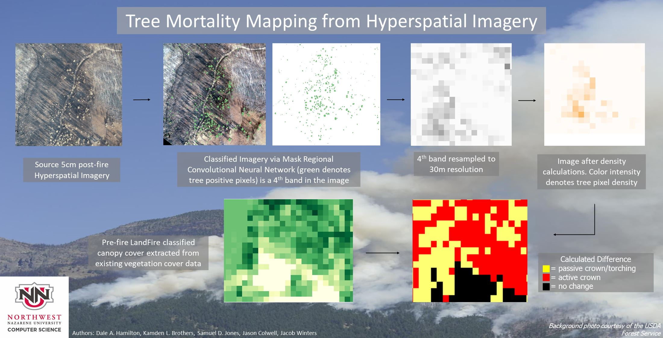
:The use of imagery from small unmanned aircraft systems (sUAS) has enabled the production of more accurate data about the effects of wildland fire, enabling land managers to make more informed decisions. The ability to detect trees in hyperspatial imagery enables the calculation of canopy cover. A comparison of hyperspatial post-fire canopy cover and pre-fire canopy cover from sources such as the LANDFIRE project enables the calculation of tree mortality, which is a major indicator of burn severity. A mask region-based convolutional neural network was trained to classify trees as groups of pixels from a hyperspatial orthomosaic acquired with a small unmanned aircraft system. The tree classification is summarized at 30 m, resulting in a canopy cover raster. A post-fire canopy cover is then compared to LANDFIRE canopy cover preceding the fire, calculating how much the canopy was reduced due to the fire. Canopy reduction allows the mapping of burn severity while also identifying where surface, passive crown, and active crown fire occurred within the burn perimeter. Canopy cover mapped through this effort was lower than the LANDFIRE Canopy Cover product, which literature indicated is typically over reported. Assessment of canopy reduction mapping on a wildland fire reflects observations made both from ground truthing efforts as well as observations made of the associated hyperspatial sUAS orthomosaic.

1. Introduction
This study investigates the use of machine learning to identify burn severity as a measure of canopy reduction. Tree crowns are classified from hyperspatial (sub-decimeter resolution) imagery using a mask region-based convolutional neural network (MR-CNN). The tree crown classification is then summarized at 30-m resolution, resulting in a canopy cover map. A post-fire canopy cover mapping product was compared to a pre-fire canopy cover mapping layer from the LANDFIRE project. The difference between the pre-fire and post-fire canopy cover enables a calculation of canopy reduction resulting as an effect of the fire, which gives an indication of tree mortality which is a primary indicator of post-fire effects resulting from a wildland fire.
Forest management practices, including fire suppression efforts, have led to forests with higher density than were found under pre-European settlement conditions. As a result, wildlands are experiencing a higher frequency of catastrophic fires, with millions of acres burned across the western US every year, often burning with much higher severity than experienced under historic conditions. These higher intensity fires result in increased incidence of soil erosion, hydrologic degradation, and deteriorating ecosystem resilience. The ability to detect trees in hyperspatial imagery enables the calculation of canopy reduction, which is a measure of wildland fire severity. The availability of canopy reduction data enables better decision making for ecosystem management and fire effect mitigation.
Background
The term “wildland fire severity” can refer to many different effects observed through a fire cycle, from how intensely an active fire is burning to the response of the ecosystem to the fire over the subsequent years. As opposed to the intensity of an active fire, which is often referred to as fire severity, this study investigates direct or immediate effects of a fire as observed in the days and weeks after the fire is contained, which we refer to as burn severity [1,2]. Previous studies in this effort examined the effect of the fire on biomass consumption which indicates how much surface vegetative material has been consumed by the fire [1,3,4,5]. By contrast, this study investigates the effect that fire has had on canopy vegetation in forested ecosystems. In situations where the amount of current post-fire canopy has not been significantly altered from what can be observed from the pre-fire conditions, it can be assumed that a fire was only consuming surface vegetation (or possibly the lower canopy) but did not consume the upper portion of the tree crowns in the canopy [6]. This low intensity fire low intensity surface fire results in no mortality of the trees in the upper canopy would result in no noticeable change of canopy cover between pre-fire and post-fire conditions. Another situation results from where all the upper tree crowns in the forest canopy have been either been consumed by a fire or the crown has been scorched by a more intense fire on the surface which extends into the tree crowns [6]. In these active crown fires, the canopy has been consumed or scorched by the fire, resulting in the death of all the trees provided that the trees are not resprouting deciduous species. This high severity active crown fire will result in a complete reduction of canopy cover as compared from pre-fire conditions. In between surface fires and crown fires, lie a situation where fire burning through surface vegetative material having enough intensity to burn or scorch the crowns of individual trees or clusters of trees, resulting in a moderate severity passive crown fire where some of the tree crowns are completely consumed or scorched [7]. While the post-fire canopy cover will be reduced from pre-fire canopy conditions as a result of these passive crown fires, the post-fire canopy cover will not be reduced to zero because some of the trees that made up the pre-fire canopy will survive, having been neither burned nor scorched.
Most land managers that use canopy cover mapping layers currently rely on the canopy cover layers that are available through the LANDFIRE project, a collaborative effort between the United States Forest Service and the US Department of the Interior. LANDFIRE produces geospatial products that describe wildland fire fuel conditions across the United States. From the LANDFIRE portal, land managers have access seamless nation-wide geospatial layers with a spatial resolution of 30 m (30 m) [8]. These canopy cover layers were generated from imagery acquired by the Enhanced Thematic Mapper Plus sensor on board the Landsat 7 satellite using a decision tree algorithm that was trained using plot data stored in the LANDFIRE Reference Database which was collected from across the US [9].
The utilization of small unmanned aircraft systems (sUAS) as a remote sensing tool provides land managers an affordable way to acquire imagery with much higher spatial resolution (sub-decimeter) than was previously available. This hyperspatial imagery produces homogeneous pixels which are comprised of a single class, resulting in higher mapping accuracy. By contrast, heterogeneous pixels which are large enough to spatially contain more than one class are common with lower resolution imagery [1,4].
Burned vegetation, unburned canopy vegetation (conifer and deciduous trees), and unburned surface vegetation (brush and grass) have been shown to have distinct spectral responses in both the visible and near infra-red spectra, though the spectral difference between canopy vegetation and surface vegetation is not as large as that between burned and general unburned vegetation [10]. This spectral difference is apparent when observing the two unburned vegetation classes in hyperspatial imagery. Persons who had participated in the acquisition of the sUAS imagery found that they could observe the visual difference between surface and canopy vegetation, with this difference in vegetation type observed in the imagery matching what they had observed in the field while conducting image acquisition flights with the sUAS.
Hamilton [1] found that tree crowns obstruct surface features in imagery acquired with a sUAS, preventing classification of surface features. Obstructed features include surface biomass consumption, a primary indicator of surface fire severity. When a tree crown is surrounded by burned surface fuel in the image, it is reasonable to assume that the ground under the tree has also burned but is obscured by the unburned crown [1,11]. Unburned tree crowns within a burned area cause an under-reporting of fire extent due to the misclassification of unburned tree crowns within the fire perimeter as being unburned areas. The first step to identifying and mapping obscured burned surface fuels is to identify trees within the image. When a tree surrounded by burned surface fuels is identified, it can be inferred that the surface fuels under the tree are in fact burned and should be included within the fire extent. Wildland fire can also affect an ecosystem through tree mortality. Mortality may result from either the ignition and consumption of a tree crown or from scorching of the tree crown caused by heat from surface fire beneath the tree. The extent of tree mortality can be estimated by calculating the change in canopy cover before and after the fire. Post-fire canopy cover can be calculated as the percentage of an image that consists of tree crowns. Pre-fire canopy cover can be retrieved from the Canopy Cover rasters that were published by the LANDFIRE Fire Fuels project [8].
2. Materials and Methods: Mapping Canopy Cover and Tree Mortality
Canopy cover describes the percentage area occupied by the upper tree crowns in forested ecosystems. In this effort, canopy cover is calculated as the percent of upper layer canopy cover within a stand, which is represented as a 30-m pixel. Once the tree crown classification has been completed, canopy cover is determined by summarizing the percentage of hyperspatial (5 cm) pixels that were classified as canopy vegetation within each 30-m Landsat pixel. Finally, the post-fire canopy cover is compared against pre-fire canopy cover from the LANDFIRE project to determine how much upper layer canopy cover reduction occurred due to the fire, giving an indication of tree mortality, which is a primary indicator of post-fire effects in forested ecosystems.
2.1. Classification of Tree Crowns from Hyperspatial Imagery
The initial step in mapping canopy cover and tree mortality enables the mapping of individual tree crowns within a hyperspatial orthomosaic acquired with the use of an sUAS. By classifying the tree crowns within an orthomosaic, we will be able to distinguish between landcover lifeforms that are indicative of canopy vegetation as opposed to surface vegetation.
The mask region-based convolutional neural network (MR-CNN) is an algorithm for instance segmentation. It detects objects in an image and determines which pixels comprise each object. When classifying an image, MR-CNN begins by applying a convolutional neural network (CNN) to extract features from the image. The features extracted from the image are used as input for a region proposal network, which slides over the feature map and detects regions of interest (RoIs) which are likely to contain objects. Each RoI is evaluated further to determine what type of object, if any, is inside (in this case, tree and non-tree); the object’s bounding box; and what pixels inside the bounding box comprise the object [12].
Training data for the MR-CNN model consists of images in which the boundaries of all trees are marked with individual polygon. Unmarked areas are assumed to be non-tree. The model is trained using mini-batch gradient descent to minimize a loss function that measures the difference between the model’s output in response to a training image and the training data.
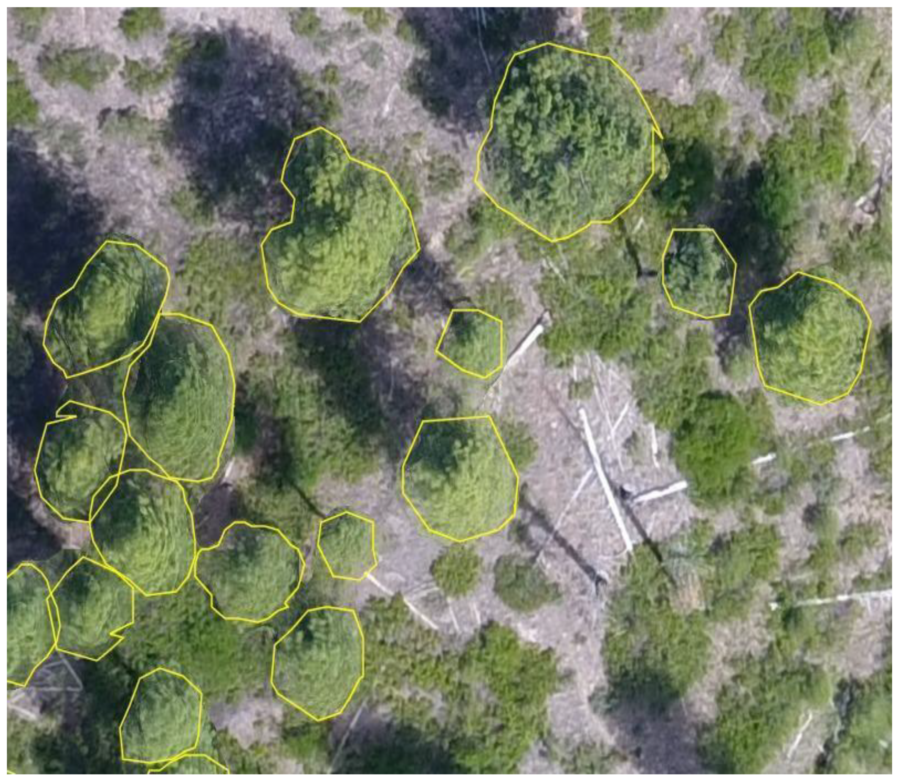
A MR-CNN model with a ResNet-101 backbone that had been pre-trained on the Microsoft COCO dataset [13] was retrained to detect trees. Training images were cropped from orthomosaics of study areas flown with sUAS over the Boise National Forest. These forested sites primarily contained Pinus Ponderosa (Ponderosa Pine), Populus Trichocarpa (Black Cottonwood), Pseudotsuga Menzieii (Douglas Fir), and Pinus Contorta (Lodgepole Pine). A polygon was traced around each tree occurring in each training image using the VGG Image Annotator [14] as shown in Figure 1. A total of 1148 trees were labeled over 14 training images. Questions of whether visually ambiguous objects were trees or surface vegetation were answered by referring to a 3D model created from the same imagery as the orthomosaics. To discourage overfitting, training images were rotated and mirrored randomly during the training process. The training data was created using many different forest types which also included images that contained scorched trees. These scorched trees were put in the “nontree” class to help the MR-CNN distinguish between burnt and non-burnt trees.
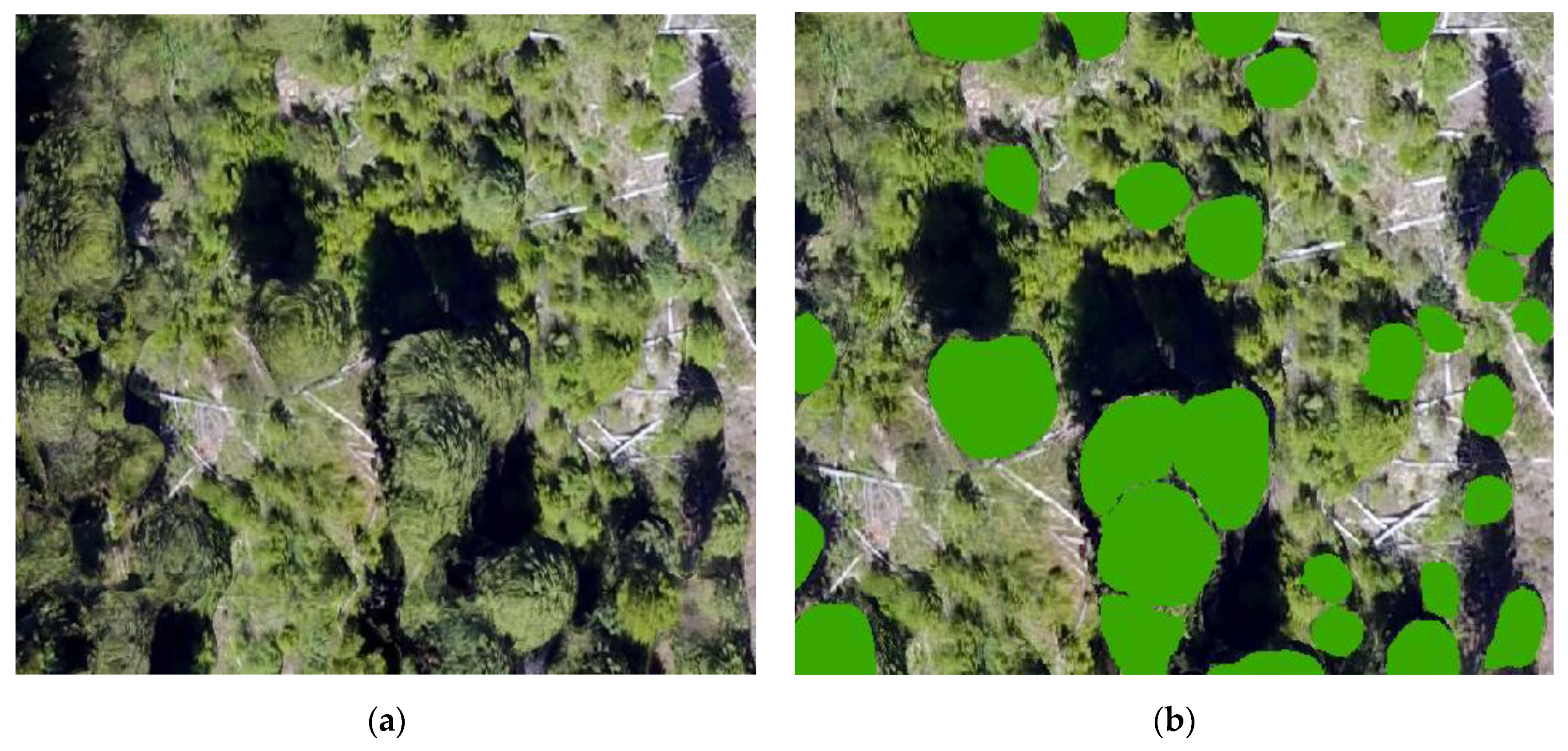
As an instance segmentation algorithm, MR-CNN can answer questions that a pixel-based approach cannot, such as, “How many trees are in the image?” and “What is the distribution of tree sizes?” To facilitate calculation of canopy cover, the MR-CNN’s output was used to perform semantic segmentation. All pixels that were determined to be part of a tree were marked as tree crown and all other pixels were marked as surface, an example of which is shown in Figure 2. Only photosynthesizing foliage was annotated in the training data for the MR-CNN, allowing the trained MR-CNN to distinguish between live trees and scorched trees, whose foliage was no longer photosynthesizing, during classification. Scorched trees would be classified as “no tree” by the MR-CNN.
2.2. Calculating Canopy Cover
Canopy cover describes the vertical projection of the tree canopy onto a horizontal plane in forested ecosystems. In this effort, canopy cover is calculated as the percent canopy cover within a stand. Once the tree crown classification has been completed as described earlier, canopy cover is determined by summarizing the percentage of 5 cm pixels that were classified as canopy vegetation within each 30-m (30 m) Landsat pixel. Because the MR-CNN is trained to only classify live trees, scorched canopy vegetation is not included in the canopy cover calculations.
2.2.1. Calculate Five Centimeter Class Densities for Each 30 Meter Pixel
The density of the tree class is calculated for each 30-m Landsat pixel from the 5 cm tree classification pixels obtained from the MR-CNN. A tool was written which calculates the density of 5 cm pixels classified as tree crown within each 30 m pixel, outputting a 30 m resolution grayscale TIFF image. This Density Tool counts the total number of hyperspatial tree class pixels occurring in the 30 m pixel. The total number of tree pixels that occurred is then divided by the total number of 5 cm pixels within the 30 m pixel and multiplied by 100. The class densities for each 30 m pixel are recorded in the class density output raster. This class density raster contains the percentage of each 30-m pixel that is comprised of 5 cm pixels that are classified as being part of a tree crown, which effectively records Canopy Cover for each 30-m pixel.
2.2.2. Canopy Cover Analysis
Previous efforts including Hamilton [1,4] and Matese [15] have shown that mapping with higher resolution imagery results in increased accuracy than using lower resolution imagery. This section summarizes the analysis performed to assess the effectiveness of the methods specified previously for calculating canopy cover.
Setting and notation: Suppose that there is a 30-m pixel depicting a region of ground. The same 30 m × 30 m region of ground is viewed as a 600 × 600 region of 5 cm pixels in the hyperspatial orthomosaic. Then the canopy cover is calculated from the hyperspatial orthomosaic, and this calculation is subject to error. The probability of correctly identifying a “tree” pixel (sensitivity) is observed from training data to be at least 0.70, and the probability of correctly identifying a “non-tree” pixel (specificity) is observed from training data to be at least 0.95. Both values are usually higher (examples are shown in Section 3.2), but we will use the values of 0.70 and 0.95 as conservative estimates.
Question: What level of accuracy can one expect for the value of canopy cover calculated from the 600 × 600 pixel region of the hyperspatial orthomosaic corresponding to a Landsat pixel? Precisely, what is the standard error of this value? Is this significantly smaller than what one might hope to obtain from LANDFIRE data?
Answer: Using The value of canopy cover can be estimated with bias close to 0 and standard error less than 0.001080. In most cases, the standard error is less than 0.000824. These values of standard error are significantly smaller than what one might hope to obtain from LANDFIRE data. They are obtained using mathematics beyond just routine statistical inference. The details are omitted here so as not to disturb the flow of the article. However, they are included in the Appendix A for the interested reader.
2.3. Canopy Cover: sUAS Derived vs. LANDFIRE
The LANDFIRE project is a collaborative effort between the United States Forest Service and the US Department of the Interior, producing geospatial products that describe wildland fire fuel conditions supporting wildland fire modeling across the United States. LANDFIRE’s Existing Vegetation Cover and Forest Canopy Cover products record the vertically projected percentage cover of the upper vegetation canopy layer [8]. For this effort in evaluating tree mortality, the Existing Vegetation Cover raster was updated to only contain canopy cover in forested ecosystems. Additionally, the Existing Vegetation Cover was updated (via the ArcGIS Spatial Analyst Con tool) with the Forest Canopy Cover for forested pixels where the predominant lifeform appeared to be either shrub or herbaceous. This conversion was accomplished by reclassing the vegetation cover for all non-forested lifeforms to zero, then substituting the Forest Canopy Cover for the Existing Vegetation Cover on pixels that had a non-forested life form, but also had a Forest Canopy Cover value. This resulted in a geospatial layer with spatial resolution of 30 m representing vertically projected percentage forest canopy cover.
The comparison of the hyperspatial derived canopy cover (HDCC) as accomplished using the ArcGIS combine raster tool. This resulted in an attribute table that had each combination of canopy cover that occurred within pixels in the two rasters as well as how many pixels the combination occurred in. From the combine table, the difference between the HDCC and LANDFIRE forest Canopy Cover (LFCC) can be calculated. This difference can be used to analyze the statistical difference between the sUAS derived and LANDFIRE products as well as the determination of canopy reduction as a measure of tree mortality in areas where the sUAS canopy cover was calculated from imagery acquired after a wildland fire.
2.3.1. Canopy Cover Comparison Methods
When classifying sUAS imagery through the Mask Regional-Convolutional Neural Network (MR-CNN), a new image is created as an output image in which pixels are based on the original image is part of a tree crown (tree) or does not comprise part of a tree crown (no tree). During this process, however, spatial referencing and null data (where a pixel represents no data) values are lost and must be added back.
Spatial referencing is added back using an ArcPy script which takes the world file spatial referencing from the original images that were aligned with the 30 m imagery, inputted into the MR-CNN and adds the spatial referencing to the MR-CNN output.
Band 4 of the classified output from the MR-CNN contains the tree/no tree classification. This band is extracted using the Copy Raster Tool on Band 4 of the image. This newly extracted classification raster is given as input to the density tool, sums the number of 5 cm tree pixels within the 30 m pixel and divides it by the total number of 5 cm pixels within a 30 m pixel. Multiplying this number by one hundred gives the percent of tree pixels or the canopy cover in the 30 m pixel area as expressed in Equation (1). This process is repeated until each pixel in the image has been analyzed giving a 30 m resolution canopy cover (CC) output raster.
Before adding the null data back into the orthomosaic, the 5-cm resolution imagery is resampled to 30 m resolution. Resampling before adding the null data speeds up the process of adding the null data back in. Null data is recorded with a pixel value of 0 (not a tree) by the MR-CNN. To restore its value to NULL, ArcPy’s conditional toolset is used to compare pixels in the source image (the MR-CNN output) and with the original data to check if the value was NULL. The density tools output is changed to 255 for every pixel where the source image’s value is NULL. To represent NULL, 255 is used because it is outside the range of possible values (0% to 100%).
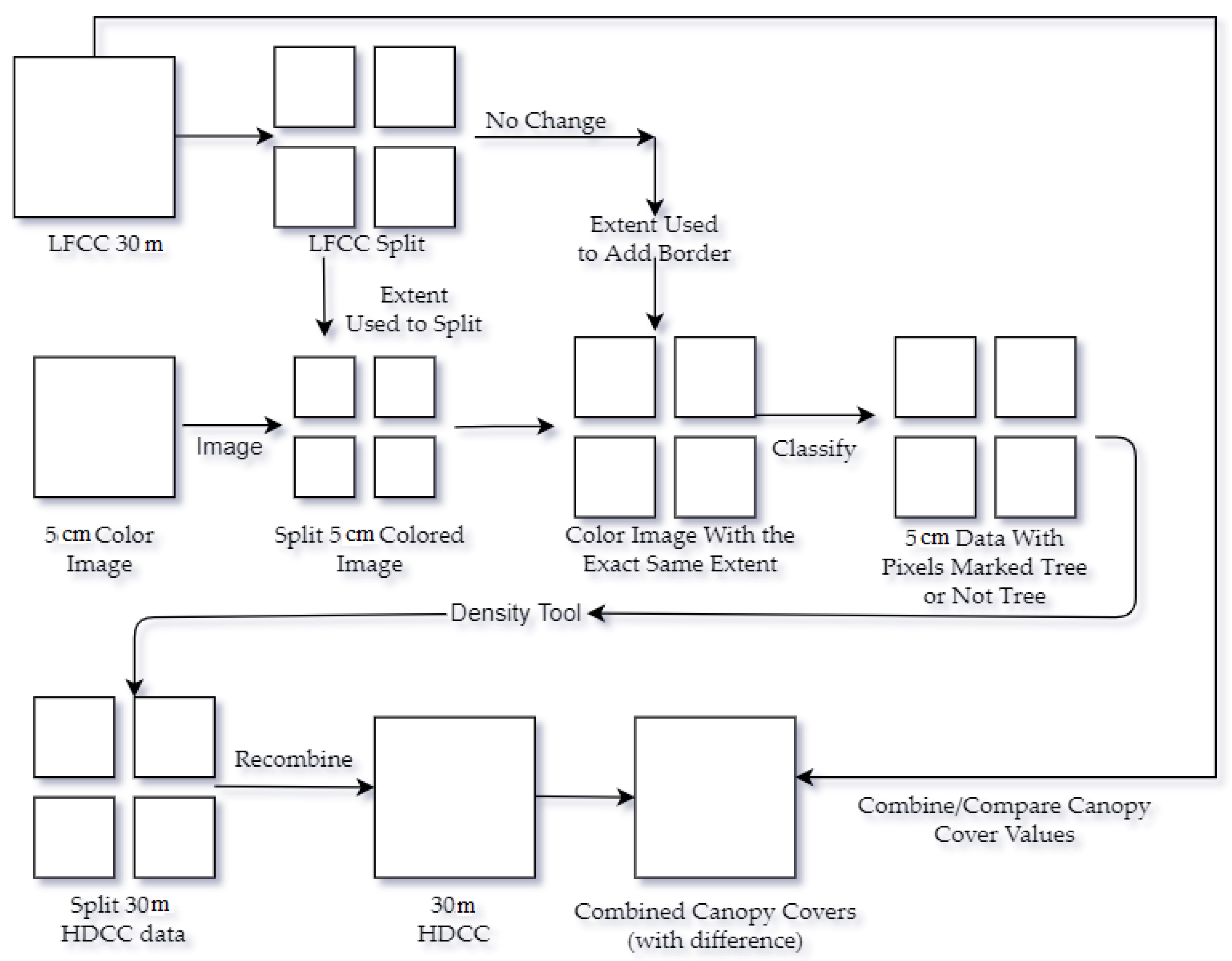
The various methods of processing the data outlined in the previous sections creates a HDCC raster that is aligned with the LFCC raster. This allows the rasters to be compared pixel by pixel, using the ArcGIS Combine Raster tool. This creates a new raster with a raster attribute table column for each of the combined rasters. Next, the LFCC column was subtracted from the HDCC column into a newly added Difference column. With sUAS data of unburned areas, this shows how close HDCC and LFCC data are. When comparing pre-fire LFCC against post-fire HDCC, this difference can be used in the calculation of canopy reduction, an indicator of tree mortality which is a primary effect of wildland fire.
The workflow which enable the calculation of the HDCC and its camparison to the LFCC is summarized in Figure 3.
2.3.2. Canopy Cover Comparison Analysis
Working assumption: In Section 2.2.2, it was observed that (assuming 5-cm pixel identification better than 0.80 correct for pixels representing ground with canopy cover, better than 0.95 for pixels representing ground without canopy cover, and no more than 0.80 canopy cover) using adjusted hyperspatial derived data, canopy cover can be calculated with a standard error of less than 0.000824. This is a much smaller standard error than we could hope to obtain from 30 m LANDFIRE pixels. Accordingly, it is reasonable, when comparing LANDFIRE data to hyperspatial derive data, to make the working assumption that the adjusted HDCC value is correct.
Objective: The method of maximum-likelihood estimation is used to construct a model of the error of the value of canopy cover derived from LANDFIRE data.
Setting and notation: There are n LANDFIRE 30 m pixels, and for each, the estimated value B ∈ [0,1] of canopy cover. For each there is a corresponding region of 5 cm pixels in the hyperspatial orthomosaic, and the adjusted value of canopy cover C ∈ [0,1] calculated from the 6002 pixels in corresponding region of the hyperspatial orthomosaic. As stated above, the latter value (C) is presumed correct, and the objective is to specify a model of the error in the former value (B). Write
for the error. The data consists of n pairs (b1, c1), (b2, c2), …, (bn, cn), from which are obtained n error values
X = B − C
x1 = b1 − c1, …, xn = bn − cn.
Model for error: A normal model for X is used, whose density is
with parameters µ (mean) and σ (standard deviation). (Note that µ and σ are the respective mean and standard deviation of the error B − C only, and not of the canopy cover itself or any estimate thereof). The values of the parameters are unknown, and the next task is to choose the best values for them (so that the model best accounts for the present data).
Maximum-likelihood estimators for parameters: The maximum-likelihood estimations for µ and σ are
and
respectively, the latter being the “population standard deviation” with denominator n instead of the “sample standard deviation” with denominator n − 1.
Conclusion: The maximum-likelihood estimation for a normal error X of the LANDFIRE value for canopy cover has mean and standard deviation , calculated from the n values x1 = b1 – c1, …, xn = bn − cn of the difference X = B − C between LANDFIRE Canopy Cover and (adjusted) Hyperspatial Derived Canopy Cover.
2.4. Mapping Tree Mortality via Canopy Reduction
While it is much more accurate to map canopy cover from hyperspatial sUAS imagery, the mapping extent is limited to how large of a study area can be flown with a sUAS. Current regulatory and technical constraints limit flight operations with a single sUAS in forested environments to under 400 hectares in a single day [16]. For mapping post-fire canopy cover, this constraint can be overcome with more flights on all but the largest fires. Due to the unpredictable nature of fires resulting from unplanned ignitions, it is not feasible to obtain hyperspatial sUAS derived canopy cover data reflecting pre-fire conditions. Fortunately, the LANDFIRE products are generated for the entire United States and are updated every two years.
For mapping canopy reduction, which is a proxy for tree mortality, a comparison was made between the LFCC (pre-fire canopy cover) against the HDCC (post-fire) layer, as described in the previous section.
Once the difference between pre-fire LFCC and post-fire HDCC, canopy cover is calculated, canopy cover reduction (CCR) can be calculated by calculating the difference between LFCC and HDCC, minus the estimated error standard deviation (multiplied by the Standard Normal density) and estimated error mean as shown in Equation (7).
2.4.1. Canopy Reduction Methods
Due to LANDFIRE’s canopy cover being less accurate than the HDCC, it cannot simply be stated that reduction is the discrepancy between sUAS Derived data and LANDFIRE data. Instead, we must use the data from unburned areas to see how much this discrepancy varies. Then any numbers outside of the normal variance is a change in canopy cover to a 95% degree of certainty. Once it is determined that there has been a change, there are two possibilities for what that change could be, active crown fire or passive crown fire. If the HDCC is 0% it was an active crown fire in this area otherwise it was a passive crown fire.
The main difficulty with calculating the type of fire based on this method is that there is some uncertainty due to LANDFIRE being 30-m data. For this reason, it is difficult to tell what happened to pixels where there was not enough of a difference to be certain if there was a change. The discrepancy between the data could just be due to LANDFIRE’s overreporting or it could be due to a passive crown fire.
2.4.2. Canopy Reduction Analysis
Working assumption: As before, a 30 m-by-30 m square of land is being considered, which corresponds to a single LANDFIRE pixel as well as to a 600 × 600 pixel region in a hyperspatial orthomosaic. Again, B ∈ [0,1] is the canopy cover according to LANDFIRE, and C ∈ [0,1] is the adjusted value of canopy cover obtained from the hyperspatial orthomosaic, which is assumed to be correct. In the previous section, maximum-likelihood estimation was used to construct a model of the error X = B − C, which was a normal density with estimated parameter values µ = = and σ = = .
Objective: A criterion is developed by which it can be concluded, with the desired level of confidence 1 − α, that canopy cover, from past LANDFIRE image to present hyperspatial orthomosaic, has decreased by at least some particular value r.
The difficulty: The difficulty here is that there is no available pre-fire value of C (canopy cover calculated from a hyperspatial orthomosaic), but only a past value of B (canopy cover calculated from LANDFIRE) to compare with the present value of C. The notation X = B − C, is still used, while now it is recognized that B is a past value and C is a present value. This means that X (difference in LFCC and (adjusted) HDCC values) may include change in canopy cover (where a positive value might result from a crown fire), or inaccuracy of LANDFIRE data, or both.
The null hypothesis: The null hypothesis that we wish to test is that there was a reduction in canopy cover of no more than r. This will be rejected if, even allowing for a canopy reduction of r, the value of B − C is too high to be explained by chance; that is, if
or, equivalently,
B − C > r + µ + zασ,
X > r + µ + zασ.
Replacing the inequality with an equality and solving for r, the following criterion is obtained.
Criterion: It may be inferred that canopy cover has decreased by at least
where B is past canopy cover according to LANDFIRE, C is the adjusted value of canopy cover from a hyperspatial orthomosaic, µ and σ are the parameter values obtained as described previously, and zα is the critical value of the Standard Normal density at significance level α. Intuitively, the amount that we can conclude by which canopy cover has been reduced is the difference “past LANDFIRE minus present hyperspatial” B − C, minus the average discrepancy µ between the LANDFIRE B and hyperspatial-derived C, minus an additional margin of error zασ which is larger, the higher the level of confidence we wish to have.
B − C − µ − zασ,
3. Results
3.1. Tree Crown Classification Validation
To assess the performance of the MR-CNN in mapping tree crowns, validation data was prepared using ArcGIS. Sample areas of canopy and surface vegetation were recorded as polygons in shapefiles digitized from existing orthomosaics. Validation data were made for all orthomosaics used in the research.
The MR-CNN was run on the orthomosaics used for validation. Agreement between a classifier’s output and the validation data was calculated using ArcMap’s Tabulate Area tool as shown in Table 1. A classifier’s accuracy on an orthomosaic was computed as the area where the classifier agreed with the class marked in the validation data divided by the total area marked in the validation data.
Orthomosaics where choose with a variety of different conditions to find any anomalies where the classifier underperforms. Trees in the chosen orthomosaics were comprised primarily of Pinus Ponderosa (Ponderosa Pine), Populus Trichocarpa (Black Cottonwood), Pseudotsuga Menzieii (Douglas Fir) and Pinus Contorta (Lodgepole Pine). All orthomosaics were from flights conducted with the Boise National Forest in southwestern Idaho [16,17]. The distinguishing characteristics of the ten chosen orthomosaics were as follows:
- NewStart: Orthomosaic consisted of 474 acres. Surface vegetation comprised of brush and herbaceous vegetation in the riparian zone along Grimes Creek. Low canopy cover.
- GrimesCreek: Orthomosaic consisted of 249 acres. Surface vegetation comprised of brush and herbaceous vegetation both inside and outside the riparian zone along Grimes Creek. Moderate to low canopy cover.
- South Placerville: Orthomosaic consisted of 262 acres. Surface vegetation comprised of brush and herbaceous vegetation both inside and outside the riparian zone. Low canopy cover.
- East Placerville: Orthomosaic consisted of 627 acres. Mix of herbaceous vegetation and canopy cover. Moderate to low canopy cover.
- West Placerville: Orthomosaic consisted of 565 acres. Wide open area covered in trees with surface vegetation along the ground around trees. Moderate to high canopy cover
- Northwest Placerville: Orthomosaic consisted of 1268 acres. Flat area with trees and tree-like brush. Moderate canopy cover.
- Edna Creek: Orthomosaic consisted of 1084 acres. Lots of unforested areas or areas with dead trees. Patches of forest throughout the orthomosaic. Low canopy cover.
- Belshazzar: Orthomosaic consisted of 265 acres. Very dense surface vegetation. Not in a riparian zone. Certain areas experienced larger-than-normal orthomosaic stitching artifacts, which we hypothesized could cause trouble for object detection techniques. Predominantly high canopy cover with some meadows.
- North Experimental Forest: Orthomosaic consisted of 800 acres. Herbaceous vegetation around water sources. Sparse forest. Moderate to low canopy cover.
- South Experimental Forest: Orthomosaic consisted of 642 acres. Not much vegetation other than trees. Ground is white in many areas. Moderate canopy cover.
The MR-CNN model’s overall accuracy was 90%. The specificity (correctly identified tree pixels/total number of tree pixels) was 84% and the sensitivity (correctly identified non-tree pixels/total number of non-tree pixels) was 99%. The MR-CNN was found to correctly identify a high number of tree pixels while only missing a low number of tree pixels as shown in Table 2.
3.2. Canopy Cover Analysis
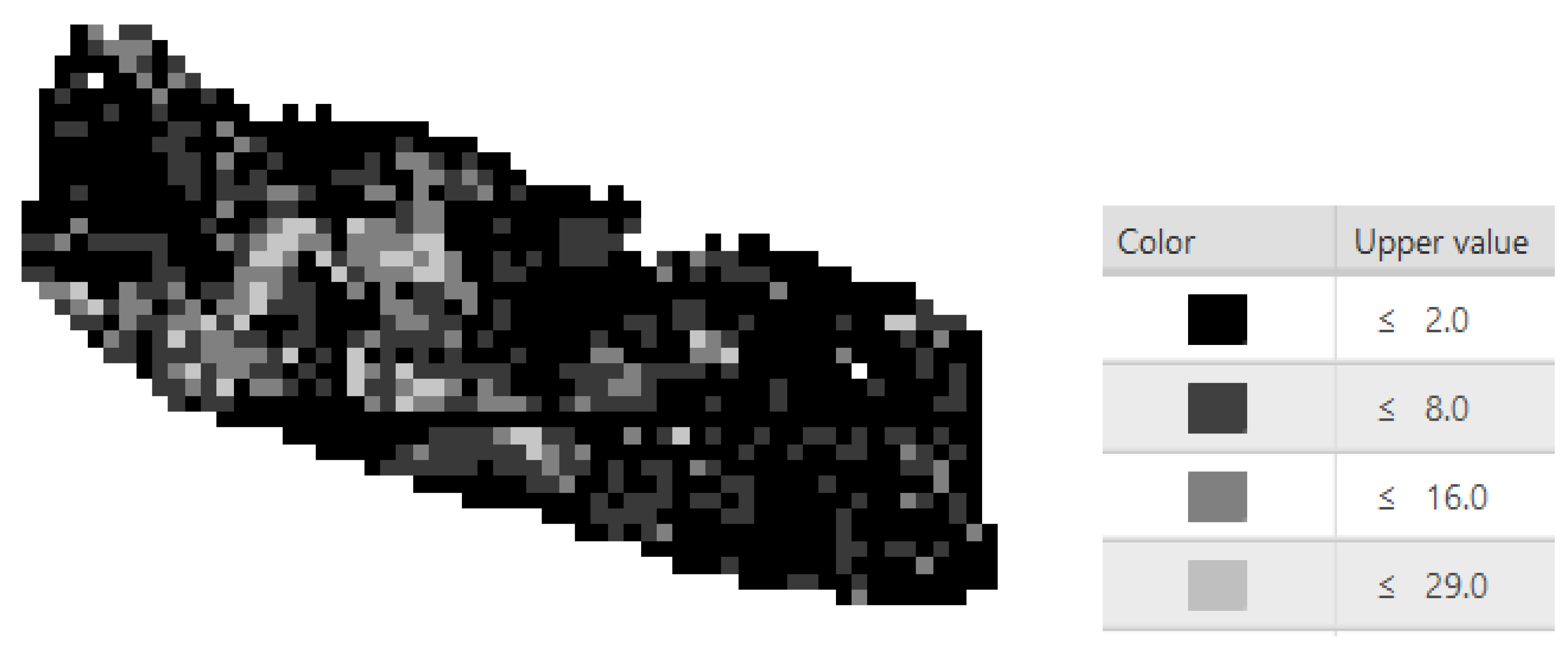
Running an orthomosaic through the Snapper Tool, MR-CNN, and Density Tool gave a 30 m orthomosaic with canopy cover that also is coregistered with LANDFIRE data. Then the HDCC numbers were adjusted based on the bias of the MR-CNN. The values used to calculate the bias were the accuracy of correctly identifying tree pixels (sensitivity) and the odds of a false positive (specificity). These numbers ended up being 84% and 99%, respectively. Figure 4 shows the HDCC layer for South Placerville.
3.3. Canopy Cover Comparison: Hyperspatial Derived vs. LANDFIRE
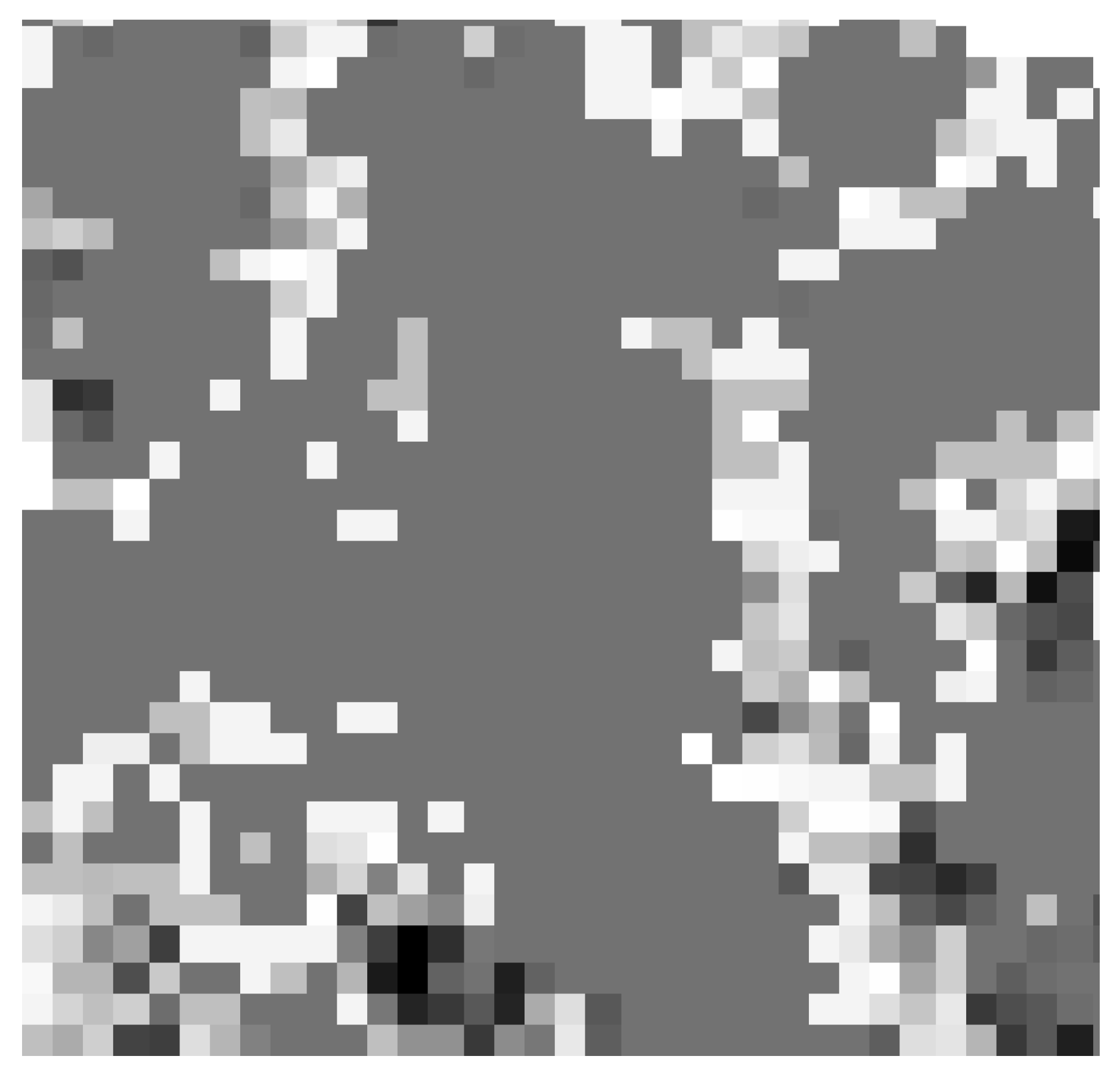
Ten orthomosaics where there was no fire were compared using the methods stated above. LANDFIRE was over reporting by an average of 2.5% over the HDCC layer. This agrees with what Scott [18] stated, that the “canopy cover values [for LANDFIRE] are too high.” The standard deviation for the difference between each pixel was 14. This number is a little high and will hopefully be driven down by future improvements. Figure 5 shows a piece of the results for Edna Creek. White represents a higher canopy cover for the HDCC layer while white represents a higher canopy cover reported by LANDFIRE. The grey composing most of the figure is for when the difference is equal or close to zero.
Table 3 shows that the LFCC over reported for every orthomosaic.
3.4. Tree Mortality Mapping Assessment
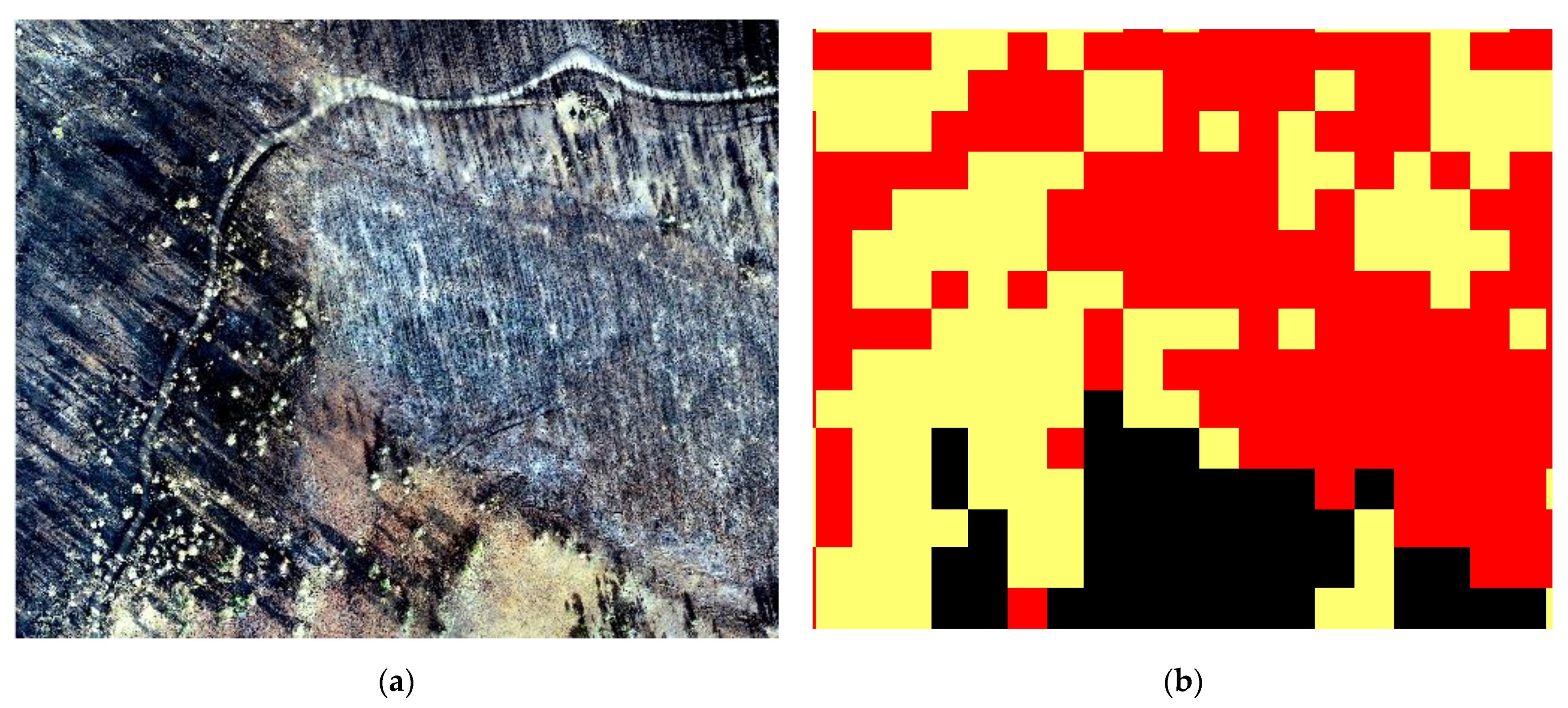
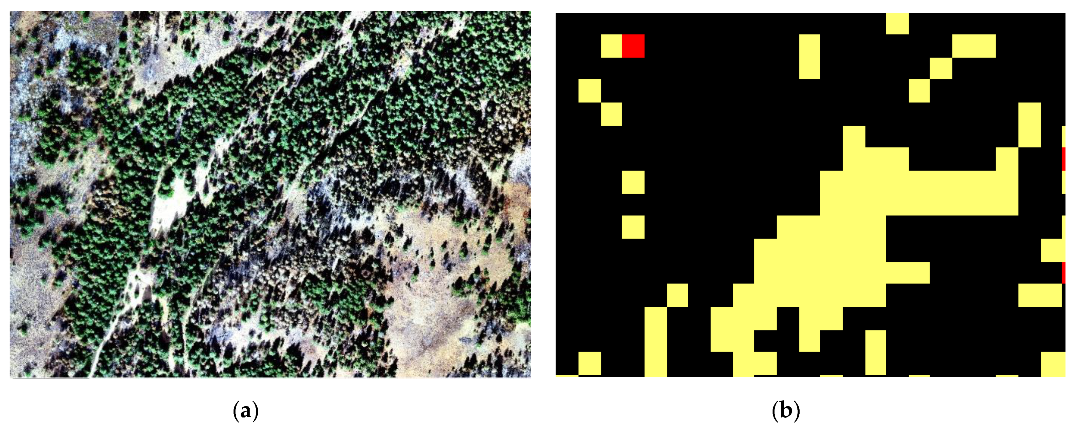
The standard deviation and mean collected from the ten non-burnt orthomosaics show that there needs to be at least a change of 27% to know there has been a change with 95% confidence. If the difference is high enough to say there has been a change next the HDCC layer can be looked at to see whether it was a passive crown fire or an active crown fire. Pixels that did not contain adequate canopy reduction (more than 26%) from comparing pre-fire LFCC to post-fire HDCC are considered to be inconclusive. This would include unburned areas, surface fire, passive crown fire, and active crown fire. If an area had less than 27% canopy cover then we cannot say whether any canopy reduction occurred. This method was used on orthomosaics acquired over portions of the Mesa fire (a 16,000-hectare mixed severity fire located on the Payette National Forest in southern Idaho) to calculate burn intensity. This fire worked well as there were areas of active crown fire, passive crown fire, and surface fire. Figure 6 shows the Southwest area of the Mesa fire which had a lot of Active Crown fire, while Figure 7 the east section which had more passive crown fire and possible surface fire.
4. Discussion
Post-fire mapping products are commonly used by land managers as they are developing post-fire management plans which specify strategies for mitigating the effects of the fire. In order for this data to be most useful, it needs to be readily available to managers. The advantage of using imagery acquired by sUAS is that it can be available as quickly as managers can get out to the site and conduct image acquisition flights. The timing of the flights can be tailored to optimize meteorological conditions that are conducive to acquiring image acquisition by enabling managers to acquire imagery as soon as the scene is not obscured by smoke and there is low enough cloud cover to ensure adequate illumination of the scene.
The MR-CNN was found to be very effective in identifying tree crowns. The classifier was found to have virtually no false positives with a specificity of 99%. The false negatives were still minimal, with a sensitivity of 84%.
Scott [18] showed that LANDFIRE Canopy Cover typically is over reported. As expected, when comparisons were made of study areas that had not experienced wildland fire, the HDCC was on average 2.5 percentage points lower than the LANDFIRE Canopy Cover. While the mean difference between the HDCC and LFCC was only a few percentage points, the higher standard deviation which typically ranged a bit more than 10 percentage points indicates that the canopy cover between the HDCC and LFCC products differed more significantly than indicated solely by the means.
The canopy reduction mapping over a burned area was very promising. When ran on the Mesa fire most pixels correctly identified surface fire as well as both active and passive crown fire. These methods work best on areas that had higher pre-fire canopy cover and canopy reduction. There needs to be at least a 27% difference for there to be a known change. Various theories to bring this number down are brought up in the future work Section 5.1.
In addition to higher accuracy mapping of canopy cover as well as tree mortality as measured by canopy reduction, the use of sUAS allows for much more current data acquisition than is possible with the LANDFIRE products. Using imagery acquired with a sUAS, it would be possible to have the HDCC product available within a day of flying a study area. By contrast, the current LANDFIRE 2.0.0 Remap effort is using Landsat imagery that was acquired in 2016. The initial product releases which covered the majority of the Contiguous US did not occur until 2019, meaning even the initial product releases were derived from imagery that was already three years out of date [8]. While canopy cover can be mapped with much higher accuracy using hyperspatial imagery acquired with a sUAS, this research team found that current technical and regulatory constraints on drone usage realistically will only allow for the acquisition of up to 600 hectares per day [16]. To effectively map large class F (>400 ha) and G (>5000 ha) fires [19], larger and more efficiently acquirable imagery satellite system still needs to be utilized to obtain a large enough analysis extent to map the whole fire. As the spatial resolution of satellite imagery increases with some of the new high-resolution sensors that are being put into orbit, it may be possible to leverage this methodology, applying it to new generations of imagery as they approach hyperspatial resolution.
5. Conclusions
Detection and mapping of trees from hyperspatial drone imagery enables more accurate mapping of canopy cover, a measure of forest density which is used to determine ecosystem departure from historic fire regimes, a primary measure of ecosystem resilience [20]. A comparison of a pre-fire LANDFIRE Canopy Cover product against post-fire HDCC resulted in a very effective measure of canopy fire reduction, which is a measure of tree mortality resulting as an effect of the wildland fire.
5.1. Future Work
While this effort was highly effective in establishing a timely, effective and cost-efficient means of mapping canopy cover and tree mortality, there are many areas of future research which could result in an improvement in the effectiveness of this methodology.
An improvement in wildland fire extent mapping can be achieved by identifying unburned trees that are surrounded by surface vegetation. Current classification methods developed through this effort [1,3] which map burn extent are not capable of detecting that a surface fire burned underneath an unburned tree crown due to the view of the surface vegetation being obscured from the sensor on the sUAS by the tree crown. While it may not be possible to determine whether the biomass consumption under the tree crown is high or low due to the presence of white ash, it would be possible to identify that the surface vegetation was burned and update the burn extent and aerial mapping accordingly based on assumptions made based on whether surface vegetation visible next to the crown was burned.
While the specificity of the MR-CNN was quite high at 99%, the accuracy of the classifier could be improved by refining the training data for the MR-CNN, based on observations of false negatives during validation. This refinement would likely improve tree crown classification, reducing the number of false negatives, thereby increasing the classifier sensitivity, which was 84% in the validation dataset used for this effort.
An improvement in tree crown classification accuracy might be able to be achieved by using pixels’ heights as additional input to the classifiers. Per-pixel height values were available from a digital surface model produced during the orthomosaic creation process but were not used as an input to the MR-CNN in this effort.
Due to the need to split each orthomosaic, the MR-CNN classifier can miss trees that are on the border of these splits since they look like half trees. This problem could be eliminated by modifying the snapping and density tool to run larger files than what they are currently limited to due to OpenCV’s file size limits. This would allow entire orthomosaics to be processed at once.
A more major problem that arises with splitting up the image is when 30 m pixels overlap. This happens because the LANDFIRE and hyperspatial image cannot line up perfectly. Because of this the 5 cm data has an extra pixel on the bottom and right when it is clipped. The density tool creates a whole 30-m pixel from these few extra 5 cm pixels on the edges. When the 30-m rasters are recombined the data at the overlap is corrupted. This problem can be fixed either creating a more direct method to handle the extra pixel or by getting rid of the split. Getting rid of the split would require OpenCV to be able to handle larger orthomosaics. This problem is most likely a big factor in the high standard deviation. If fixed, the difference needed to be confident there has been a change should drop.
Author Contributions
Conceptualization, D.A.H.; Methodology, D.A.H., K. Brothers, S.D.J., J.W.; software, D.A.H., K.L.B., S.D.J., J.W.; validation, K.L.B.; formal analysis, J.C.; investigation, D.A.H., K.L.B., S.D.J.; data curation, D.A.H.; writing, D.A.H., J.C., K.L.B., S.D.J., J.W.; visualization, K.L.B.; supervision, D.A.H.; project administration, D.A.H.; funding acquisition, D.A.H. All authors have read and agreed to the published version of the manuscript.
Funding
This research was funded by the USDA Forest Service Boise National Forest, Forest Service Agreement No, 18-CS-11040200-0025.
Institutional Review Board Statement
Not applicable.
Informed Consent Statement
Not applicable.
Data Availability Statement
All data and source code from this project is available at the https://firemap.nnu.edu/tree-mortality.
Acknowledgments
We would like to acknowledge the students in the Northwest Nazarene University Department of Math and Computer Science who have helped with different aspects of this effort, including current and former students Nicholas Hamilton, Jonathan Hamilton, Braelyn Boerner, Gabriel Murphy, Enoch Levandovsky, Gabriel Johnson, Austin White, Aleesha Chavez and Andrew Welk. Additionally, we would like to acknowledge Northwest Nazarene University who funded the research efforts of many of the students mentioned.
Conflicts of Interest
The authors declare no conflict of interest.
Appendix A. Accuracy of Calculated Value for Canopy Cover
In this appendix, the accuracy of the value for canopy cover calculated from the hyperspatial orthomosaic is shown to be better than that calculated from LANDFIRE. This conclusion was stated in Section 2.2.2, but depends on mathematics beyond just routine statistical inference. The details are given here to justify the conclusion.
Setting and notation: Suppose that there is a 30 m pixel depicting a region of ground with canopy cover value c ∈ [0,1]. The actual value c would be unknown in practice. The same 30 m × 30 m region of ground is viewed as an region of smaller pixels in the hyperspatial orthomosaic. In practice, would be equal to 600, and the 600 × 600 orthomosaic would consist of 5 cm pixels, but the symbol will be used for now for greater clarity.) The number of true “tree” pixels is , and the number of “non-tree” pixels is . Each of the pixels is assigned by the MR-CNN a binary value A = 1 (tree) or A = 0 (non-tree). Then the canopy cover is calculated from the hyperspatial orthomosaic as
where the sum is taken over all pixels.
The assignments are subject to error. Suppose the probability of correctly assigning A = 1 to a “tree” pixel (sensitivity) is known to be p ∈ [0,1], and the probability of correctly assigning A = 0 to a “non-tree” pixel (specificity) is known to be q ∈ [0,1].
Question: What level of accuracy can one expect for the value of canopy cover calculated from the pixel region of the hyperspatial orthomosaic corresponding to a Landsat pixel? Precisely, what is the standard error of this value? Is this significantly smaller than what one might hope to obtain from LANDFIRE data?
Mean and standard deviation of calculated value: The expected value (mean) of the calculated value is
The standard deviation is
Adjustment of value for canopy cover: Recall that c is the proportion of small pixels representing ground that has canopy cover. It is the number wanted but not known. One solves for c in the expression for above to obtain
and thus
is an unbiased estimator of c. This will be called the “adjusted canopy cover”. The standard error of C is just the standard deviation of divided by , which is
Next, this expression will be examined more closely to obtain an upper bound.
Derivation of upper bound: The quantity x(1 − x) is decreasing for on the interval .
So that since p > 0.70 and q > 0.95,
p(1 − p) < (0.70)(1 − 0.70) and q(1 − q) < (0.95)(1 − 0.95).
It also follows that
whereupon
(which is a weighted mean of (0.70)(1 − 0.70) and (0.95)(1 − 0.95)) is an increasing function of c. Combining this fact with the first two inequalities, one obtains
for
(0.70)(1 − 0.70) > (0.95)(1 − 0.95),
c(0.70)(1 − 0.70) + (1 − c)(0.95)(1 − 0.95)
| cp(1 − p) + (1 − c)q(1 − q) |
| < c(0.70)(1 − 0.70) + (1 − c)(0.95)(1 − 0.95) |
| < (0.80)(0.70)(1 − 0.70) + (1 − 0.80)(0.95)(1 − 0.95) |
p > 0.70, q > 0.95, and c < 0.80.
The actual canopy cover (c) in the training data used was less than 0.80, the sensitivity (p) was better than 0.70, and the specificity (q) better than 0.95. Using also , one obtains
which compares favorably with results obtained with LANDFIRE 30 m pixels. If one assumes that p > 0.80 (which is true in most cases) rather than merely p > 0.70, the upper bound on the standard error of C becomes
which would be impossibly low to achieve with LANDFIRE 30 m pixels.
Conclusion: The adjusted value of canopy cover calculated from the hyperspatial orthomosaic has lower standard error than we could hope to obtain from LANDFIRE 30-m pixels.
References
- Hamilton, D. Improving Mapping Accuracy of Wildland Fire Effects from Hyperspatial Imagery Using Machine Learning. Ph.D. Thesis, University of Idaho, Moscow, ID, USA, 2018. [Google Scholar]
- Keeley, J.E. Fire intensity, fire severity and burn severity: A brief review and suggested usage. Int. J. Wildl. Fire 2009, 18, 116–126. [Google Scholar] [CrossRef]
- Hamilton, D.; Pacheco, R.; Myers, B.; Peltzer, B. kNN vs. SVM: A Comparison of Algorithms. In Proceedings of the Fire Continuum—Preparing for the Future of wildland Fire; Missoula, MT, USA, 21–24 May 2018, p. 358. Available online: https://www.fs.usda.gov/treesearch/pubs/60581 (accessed on 1 December 2020).
- Hamilton, D.; Hamilton, N.; Myers, B. Evaluation of Image Spatial Resolution for Machine Learning Mapping of Wildland Fire Effects. In Proceedings of SAI Intelligent Systems Conference; Springer: Cham, Switzerland, 2019; pp. 400–415. [Google Scholar]
- Hamilton, D.; Myers, B.; Branham, J. Evaluation of Texture as an Input of Spatial Context for Machine Learning Mapping of Wildland Fire Effects. Signal Image Process. Int. J. 2017, 8, 146–158. [Google Scholar] [CrossRef]
- Rothermel, R.C. Predicting Behavior and Size of Crown Fires in the Northern Rocky Mountains; U.S. Department of Agriculture, Forest Service, Intermountain Forest and Range Experiment Station: Ogden, UT, USA, 1991.
- Cruz, M.G. Development and testing of models for predicting crown fire rate of spread in conifer forest stands. Can. J. For. Res. 2005, 35, 1626–1639. [Google Scholar] [CrossRef]
- LANDFIRE. Landfire Program. 2020. Available online: https://landfire.gov/ (accessed on 25 November 2020).
- Reeves, M.C.; Ryan, K.C.; Rollins, M.G.; Thompson, T.G. Spatial fuel data products of the LANDFIRE Project. Int. J. Wildl. Fire 2009, 18, 250. [Google Scholar] [CrossRef]
- Hamilton, D.; Bowerman, M.; Collwel, J.; Donahoe, G.; Myers, B. A Spectroscopic Analysis for Mapping Wildland Fire Effects from Remotely Sensed Imagery. J. Unmanned Veh. Syst. 2017, 5, 146–158. [Google Scholar] [CrossRef] [PubMed] [Green Version]
- Scott, J.H.; Reinhardt, E.D. Assessing crown fire potential by linking models of surface and crown fire behavior. In USDA Forest Service Research Paper; USDA: Fort Collins, CO, USA, 2001; p. 1. [Google Scholar]
- He, K.; Gkioxari, G.; Dollar, P.; Girshick, R. Mask R-CNN. In Proceedings of the IEEE International Conference on Computer Vision, Venice, Italy, 22–29 October 2017. [Google Scholar]
- Lin, T.Y.; Maire, M.; Belongie, S.; Hays, J.; Perona, P.; Ramanan, D.; Dollár, P.; Zitnick, C.L. Microsoft COCO: Common objects in context. In European Conference on Computer Vision; Springer: Cham, Switzerland, 2014; pp. 740–755. [Google Scholar]
- Dutta, A.; Zisserman, A. The VIA Annotation Software for Images, Audio and Video; Springer: New York, NY, USA, 2019. [Google Scholar] [CrossRef] [Green Version]
- Matese, A.; Toscano, P.; Di Gennaro, S.F.; Genesio, L.; Vaccari, F.P.; Primicerio, J.; Belli, C.; Zaldei, A.; Bianconi, R.; Gioli, B. Intercomparison of UAV, aircraft and satellite remote sensing platforms for precision viticulture. Remote Sens. 2015, 7, 2971–2990. [Google Scholar] [CrossRef] [Green Version]
- Goodwin, J.; Hamilton, D. Archaeological Imagery Acquisition and Mapping Analytics Development; Boise National Forest: Boise, ID, USA, 2019.
- Calkins, A.; Hamilton, D. Archaeological Imagery Acquisition and Mapping Analytics Development; Boise National Forest: Boise, ID, USA, 2018.
- Scott, J. Review and Assessment of LANDFIRE Canopy Fuel Mapping Procedures. LANDFIRE, LANDFIRE Bulletin. 2008. Available online: https://landfire.cr.usgs.gov/documents/LANDFIRE_Canopyfuels_and_Seamlines_ReviewScott.pdf (accessed on 30 July 2020).
- National Wildfire Coordinating Group (NWCG). Size Class of Fire. 2020. Available online: www.nwcg.gov/term/glossary/size-class-of-fire (accessed on 20 May 2020).
- Barrett, S.; Havlina, D.; Jones, J.; Hann, W.; Frame, C.; Hamilton, D.; Schon, K.; Demeo, T.; Hutter, L.; Menakis, J.; et al. Interagency Fire Regime Condition Class Guidebook; Version 3.0; USDA Forest Service, US Department of Interior, and The Nature Conservancy: Rolla, MO, USA, 2010.
Figure 1.
Mask Region-based Convolutional Network training data.

Figure 2.
(a) is pre-classified image. (b) is an image that has been classified by the MR-CNN.

Figure 3.
An overview of the processes used to create the HDCC.

Figure 4.
Values are in percent canopy cover.

Figure 5.
A raster representing the comparison between the LANDFIRE and HDCC data. White means LANDFIRE reported more canopy cover while black indicates the inverse.
Figure 5.
A raster representing the comparison between the LANDFIRE and HDCC data. White means LANDFIRE reported more canopy cover while black indicates the inverse.

Figure 6.
(a) Hyperspatial data after a burn. (b) Types of fire: Red = Active, Yellow = Passive, Black = inconclusive crown fire activity.
Figure 6.
(a) Hyperspatial data after a burn. (b) Types of fire: Red = Active, Yellow = Passive, Black = inconclusive crown fire activity.

Figure 7.
(a) Hyperspatial data after a burn. (b) Types of fire: Red = Active, Yellow = Passive, Black = inconclusive crown fire activity.
Figure 7.
(a) Hyperspatial data after a burn. (b) Types of fire: Red = Active, Yellow = Passive, Black = inconclusive crown fire activity.


Table 1.
Confusion matrices of MR-CNN tree crown classifications. Classified surface and canopy are shown in the rows while human labeled surface and canopy are in columns.
Table 1.
Confusion matrices of MR-CNN tree crown classifications. Classified surface and canopy are shown in the rows while human labeled surface and canopy are in columns.
| South Placerville | NW Placerville | Edna Creek | South Exp. Forest | |||||
|---|---|---|---|---|---|---|---|---|
| Surface | Canopy | Surface | Canopy | Surface | Canopy | Surface | Canopy | |
| Surface | 47.5% | 19.9% | 46.6% | 6.2% | 49.0% | 0.6% | 49.1% | 10.6% |
| Canopy | 0.6% | 32.0% | 2.3% | 44.9% | 0.0% | 50.3% | 0.4% | 40.0% |
| North Exp. Forest | East Placerville | West Placerville | ||||||
| Surface | Canopy | Surface | Canopy | Surface | Canopy | |||
| Surface | 50.0% | 10.5% | 49.29% | 4.50% | 49.98% | 7.29% | ||
| Canopy | 0.3% | 39.2% | 0.00% | 46.21% | 0.00% | 42.73% | ||
| Belshazzar | Newstart | Grimes Creek | ||||||
| Surface | Canopy | Surface | Canopy | Surface | Canopy | |||
| Surface | 47.1% | 3.6% | 50.1% | 16.9% | 51.5% | 2.9% | ||
| Canopy | 3.0% | 46.3% | 0.2% | 32.8% | 0.2% | 45.4% | ||
Table 2.
MR-CNN tree crown classification statistical summary.
| Accuracy | Specificity | Sensitivity | |
|---|---|---|---|
| South Placerville | 79.5% | 98.2% | 70.5% |
| NW Placerville | 91.5% | 95.1% | 88.3% |
| Edna Creek | 99.3% | 100.0% | 98.8% |
| South Exp. Forest | 89.1% | 99.0% | 82.2% |
| North Exp. Forest | 89.2% | 99.2% | 82.6% |
| East Placerville | 95.5% | 100.0% | 91.6% |
| West Placerville | 92.7% | 100.0% | 87.3% |
| Belshazzar | 93.4% | 93.9% | 92.9% |
| Newstart | 82.9% | 99.4% | 74.8% |
| Grimes Creek | 96.9% | 99.6% | 94.7% |
Table 3.
Mean difference and the standard deviation of that difference for each area.
| Mean | Standard Deviation | |
|---|---|---|
| Belshazzar | 17% | 14 |
| New Start | 4% | 13 |
| Grimes Creek | 6% | 15 |
| NW Placerville | 1% | 11 |
| 0530 Placerville | 10% | 9 |
| Edna Creek | 4% | 1 |
| South Experimental Forest | 3% | 12 |
| North Experimental Forest | 7% | 12 |
| East Placerville | 7% | 12 |
| West Placerville | 2% | 13 |
Publisher’s Note: MDPI stays neutral with regard to jurisdictional claims in published maps and institutional affiliations. |
© 2021 by the authors. Licensee MDPI, Basel, Switzerland. This article is an open access article distributed under the terms and conditions of the Creative Commons Attribution (CC BY) license (http://creativecommons.org/licenses/by/4.0/).
Share and Cite
MDPI and ACS Style
Hamilton, D.A.; Brothers, K.L.; Jones, S.D.; Colwell, J.; Winters, J. Wildland Fire Tree Mortality Mapping from Hyperspatial Imagery Using Machine Learning. Remote Sens. 2021, 13, 290. https://doi.org/10.3390/rs13020290
AMA Style
Hamilton DA, Brothers KL, Jones SD, Colwell J, Winters J. Wildland Fire Tree Mortality Mapping from Hyperspatial Imagery Using Machine Learning. Remote Sensing. 2021; 13(2):290. https://doi.org/10.3390/rs13020290
Chicago/Turabian StyleHamilton, Dale A., Kamden L. Brothers, Samuel D. Jones, Jason Colwell, and Jacob Winters. 2021. "Wildland Fire Tree Mortality Mapping from Hyperspatial Imagery Using Machine Learning" Remote Sensing 13, no. 2: 290. https://doi.org/10.3390/rs13020290
Note that from the first issue of 2016, this journal uses article numbers instead of page numbers. See further details here.