A Preliminary Study of Wave Energy Resource Using an HF Marine Radar, Application to an Eastern Southern Pacific Location: Advantages and Opportunities

Abstract

As climate change is of global concern, the electric generation through fossil fuel is progressively shifted to renewable energies. Among the renewables, the most common solar and wind, the wave energy stands for its high-power density. Studies about wave energy resource have been increasing over the years, especially in coastal countries. Several research investigations have assessed the global wave power, with higher values at high latitudes. However, to have a precise assessment of this resource, the measurement systems need to provide a high temporal and spatial resolution, and due to the lack of in-situ measurements, the way to estimate this value is numerical. Here, we use a high-frequency radar to estimate the wave energy resource in a nearshore central Chile at a high resolution. The study focuses near Concepción city (36.5° S), using a WERA (WavE RAdar) high frequency (HF) radar. The amount of annual energy collected is calculated. Analysis of coefficient of variation (COV), seasonal variability (SV), and monthly variability (MV) shows the area’s suitability for installing a wave energy converter device due to a relatively low variability and the high concentration of wave power obtained. The utility of HF radars in energy terms relies on its high resolution, both temporal and spatial. It can then compare the location of interest within small areas and use them as a complement to satellite measurements or numerical models, demonstrating its versatility.

1. Introduction

Worldwide marine energies have been widely studied. Recent work [1,2,3,4,5] establishes a more significant wave potential at higher latitudes. The most favored coasts being, to name only a few, Australia, New Zealand, South Africa, Chile, the western U.K., and Canada. Wave devices are currently lagging tidal in terms of technological development. As many as 170 types of wave energy converter have been designed, fewer than 20% are at the full-scale prototype stage [6]. By 2017, the world’s installed capacity for marine energy was 536 MW, compared to 267 MW in 2007 [7]. However, Ocean Energy Europe has projected at a low grown scenario that 1300 MW of tidal energy and 170 MW of wave energy could be installed by 2030 [8].

Chile is one of the countries with the most extensive maritime territory, with a coastline that extends from 19° S to 56° S, positioning it as one of the best countries to develop wave energy. Marine gravity waves are considered one of the coastal ocean’s essential features due to their impact on security issues such as harbor activities, traffic planning, beach management, and energy potential. It is vital to have constant monitoring of the ocean, especially when a strong presence of coastal industrial and residential activity is present.

Several methodologies, numerical or instrumental, provide relevant information of waves, either in-situ (buoys), remotely (radars, satellites), or through computational models—the set of methodologies and instruments constituting an integrated observation system [9]. Remote instruments deliver information from the study area on a large scale through data acquired by a device that is not in contact with what is being investigated [10]. It is of great importance for ocean data since the environment can be quite hostile and ample to be covered with in-situ instruments. The most used are satellites that cover a large part of the Earth, and for which information is available since the early 90s [11].

Other instruments of remote sensing are the high-frequency marine radars. They are located on the coastline and study oceanographic variables providing high spatial and temporal coverage. These systems’ applicability includes port security, tsunami detection, renewable energy, storm surges, and flooding, among others [12,13,14,15,16,17]. The advantage of using HF radars instead of instruments such as buoys or satellites is their high spatial coverage. It is also possible to complement satellites’ information with the radar information (which does not provide quality measurements near the coastal area [18]). The HF radar range can be up to 100 km from the coast.

The best option to measure wave by HF radars is through a dual system. Two radars sweep a shared area, illuminating each surface water parcel from two directions, thus avoiding ambiguities when measuring the wave height [19]. The same work compares data from single and dual HF radar systems: It shows that the dual radar algorithm is significantly more accurate and reliable. One consideration to have in mind is that single or dual radar measurements tend to be less accurate in high sea states because of limitations in the backscatter model in these conditions [19]. More precisely, Ref. [20] shows that the HF radar wave height’s accuracy is around 12.6%. However, one radar does obtain significant wave height with a range of approximately 30 km from the coast [12,13,21]. A single radar can be used in particular applications to look directly into the operationally-important wave propagation [20] and always as a complement to other instruments.

The use of HF marine radars is not uncommon in first-world countries (United States, Europe, Australia, and Japan [22]. In other countries, however, their use is somewhat limited. For example, Mexico and Chile use these systems in the rest of the American continent [23] (see Section 2.1).

Considering the wave energy opportunities in Chile, this work aims to present a preliminary study of an HF marine radar application. Our goal is to assess the wave energy potential and prove the usefulness of this instrument to establish the wave energy resource of a specific location. This way, we can provide a high-resolution grid to determine specific hotspots that could optimize the available energy harness.

2. Materials and Methods

2.1. Study Area and Data

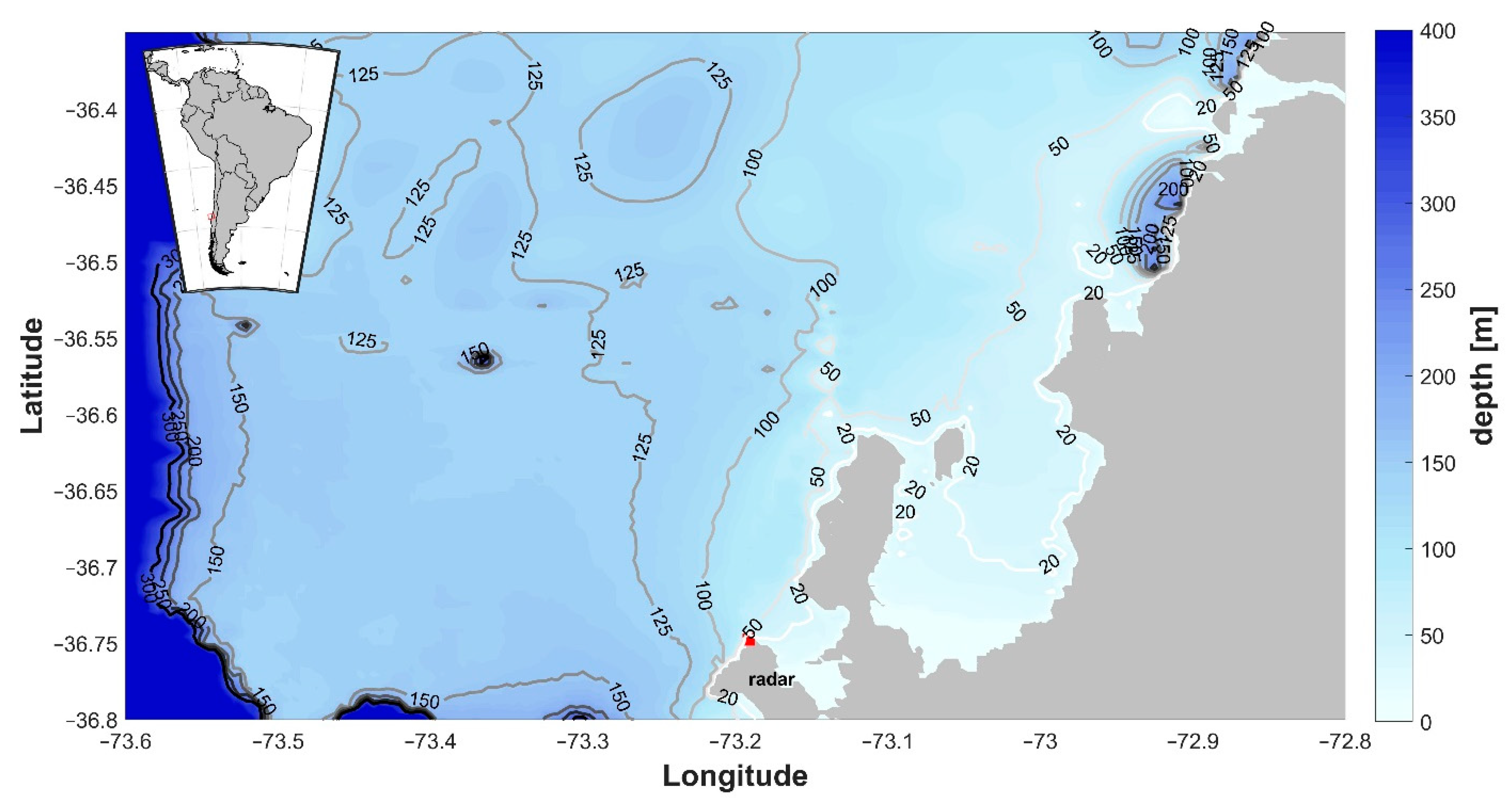
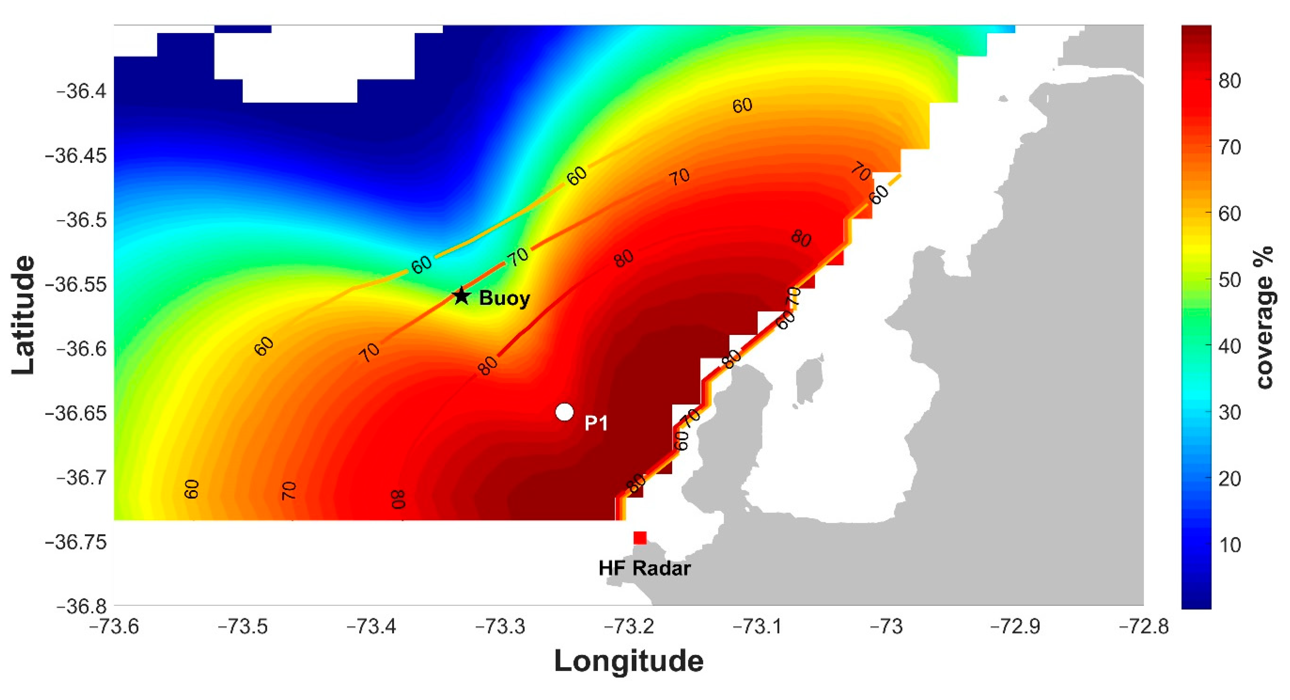
2.1.1. Study Area

The study site is located in south-central Chile’s coastal area facing the Pacific Ocean (Figure 1). The continental shelf is approximately 100 m deep and extends about 60 km west to 73.5° W. The red dot in Figure 1 shows the location of the radar used in the present study. Information from a global climatology [24], as specific data from the zone [25], indicates that the wave height has a uniform spatial pattern with average values close to 3 m and lowest variability [26] and typical periods between 9 and 12 s [25]. The winds in this area come predominantly from the southwest [25], impacting the wave’s direction.

2.1.2. HF Marine Radar

Wave measurements in front of the Bío-Bío region were made by a WERA HF radar [12], working at a frequency of 16.15 MHz. It is located in the "Faro Hualpén" Bío-Bío region (36.74° S–73.19° W). The system has four (4) transmitting and eight (8) receiving antennas. It has a sampling frequency of 33 s. The maximum range is 100 km, with an aperture of +/− 50° spatial resolution of 2 km and an azimuthal resolution of 4°.

The waves were measured in a regular grid of 2 km resolution and a temporal interval of 1 h. For this study, we used approximately one year of measurements between December 2017 and January 2019.

This radar is part of the ocean observation system CHIOOS (www.chioos.cl) in charge of the Department of Geophysics (DGEO) of the University of Concepción (UDEC). It is the only HF radar in the entire southeast Pacific coast [23] and, together with those located in Australia [22], to the best of our knowledge, the only ones in the South Pacific.

2.2. Methodology

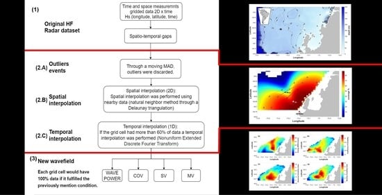
2.2.1. Data Processing

The radar sweep area is not constant throughout the study period. There were times when no measurement took place, having more of fewer grid cell to be studied. Although the same area is always covered, the amount of spatial data is not the same. Moreover, the further away from the radar, the lower the spatial coverage and the quality of the data. Although the radar area varies at each measurement time, the measured points are grouped in the same area and not scattered throughout the sweep. It generates both spatial and temporal discontinuity in the data. Figure 2 display a flow chart that resumes the data treatment process. It is divided into 3 main parts. The 1st represents the initial dataset state. The 2nd division is the data processing performed; this involves 3 stages (A, B, and C). The first part was the suppression of extreme elements (A), two interpolation parts (B: 2D and C: 1D), and the 3rd the dataset obtained.

Radar measurements showed noise and outliers, with extreme values exceeding 3 or even 5 standard deviations (see Figure 5), exceptionally with hourly waves as high as 10–13 m, even close to the coast. The region’s wave height for those dates was verified by checking with the only buoy in the area and analyzing the Chilean navy’s information for those times. In the end, for those epochs, the radar reported erroneous peaks. Therefore, to eliminate outliers, the gridded time series were first filtered by a 3-day moving median [27]. All the data above or below the 1.5 MAD were discarded. It generated a cleaner data field and time series without those extreme values (2A stage in Figure 2). Then, in order to have a coherent space-time data field, we performed a spatial-temporal interpolation (see stages 2B and 2C in flow diagram, Figure 2). When the grid point met the natural neighbor 2D interpolation specific applicability conditions (employing a natural neighbor method through a Delaunay triangulation [28]), spatial interpolation was executed. It allowed filling empty grid points with surrounding radar measurements (stage 2B in Figure 2). However, despite the spatial interpolation, there were still grid points with temporal gaps. On average, only 15% of the data was filled because of these restrictions. Then, in those places where there were still missing data, we performed a temporal interpolation applying a Nonuniform Extended Discrete Fourier Transform [29,30]. It is applied only if the grid complies with the condition that there were more than 60% of the data (see stage 2C in Figure 2).

Note that, interpolating solely by 1D (time), crude discontinuities may appear in both time and space. Thus, if each grid cell time series is treated as an independent time series, it creates many spatial discontinuities, which may well not represent the reality of the spatial variability within the area interpolated. Inversely, spatial interpolation followed by 1D (time) interpolation ensures the field variability’s spatial continuity is preserved.

The interpolation method, as the methodology of temporal interpolation through different ways, was verified. For example, comparing the interpolation made in the buoy or the radar series that had a greater number of original points. The interpolation technique for missing data that most preserves the data’s reality is the Nonuniform Extended Discrete Fourier Transform [29,30] method. Thus, the grid points that did not have data before and after the spatial interpolation were subtracted. Then, the correlation between the original buoy series and the temporal interpolated buoy series was calculated. On the buoy, the correlation was 0.81 and 0.86, respectively. Next, the same test was performed with the radar series that was initially the most complete; 88% of the data and 15 kilometers off the coast (location 73.1665° W, 36.6441° S). In this case, the correlation was 0.864 and 0.858. In summary, this shows that the method of temporal interpolation used is sufficiently robust.

Figure 3 shows the radar’s sweep coverage area, between 36.2° S–36.7° S and 73.0° W–73.6° W. The percentage of the radar’s original coverage is also shown as a data field. The final percentage after spatial interpolation is shown in contour lines. Blue/red color shows the places with less/more than average data. From the coast (oblique) to 30 km offshore (i.e., the equivalent of 0.27 degrees), it has 60 to 80% spatial coverage (red to orange colors) of the data for one year of study. Further away from this area, it has the worst coverage, between 40 and 10% of data (blueish colors). So we will only focus on the first 30 km.

The treatment previously mentioned allowed the construction of a regular spatial-temporal grid data set. That is, 20 latitude × 28 longitude points (corresponding to 560 grid points), with a spatial resolution of 2 km and 9444 hourly time points from December 2017 to January 2019). Statistics in Figure 2 are derived from the interpolated fields.

2.2.2. Wave Potential

Once the data set is complete, the wave potential, energy period, coefficient of variation, and seasonal and monthly variability coefficients are calculated [1]. These parameters are essential to establish the locations where the extraction of energy is favorable either by having a high potential or a low variability, or a combination of both [31].

For the calculation of the potential, the following equation in W/m was used, which is valid for deep waters, $h>\frac{\lambda }{2}$ [32,33]

$$P=\rho g\frac{H_s^2{T}_e}{64\pi }$$

(1)

where $\rho$ is the density of seawater (1027 $\mathrm{kg}/{\mathrm{m}}^3$), $g$ is the acceleration due to gravity (9.81 m/s²), $H_s$ is the significant wave height in meters, and $T_e$ being the energy period in seconds. It is the period of a monochromatic wave that contains the same mean energy as the rough sea [34]. The HF radar gives the wave height. However, the radar’s measurements do not provide all the information required to obtain the energy period.

The wave energy period can be calculated from the wave spectra ($S\left(f\right)$) as [34]

$$Te=\frac{m_{-1}}{m_o}$$

(2)

where the nth spectral moment is defined as

$$m_n={{\displaystyle \int }}_0^{\infty }{f}^{n}S\left(f\right) df$$

(3)

Ref. [1] specifies that $T_e$ should be estimated from other variables when the spectral form is unknown. Therefore, we will use the peak period $(T_p)$ estimated in previous works [24,25,35], as

$$T_e=0.9 T_p$$

(4)

The use of a bibliographic value lies in the lack of correlation between the HF radar and in-situ information (see below Section 3). This way, the wave power calculation would be more representative and robust (this topic is discussed in more detail in Section 4). For this area, the peak period is around 10 s (e.g., Chilean wave atlas [35]). Although the value of $T_e$ is constant and does not vary throughout the year of study, it is expected that the errors associated with the period are not significant compared to the wave height because $P\propto T_e{H}_{s }^2$ [1,36]

The coefficient of variation (COV) [1,37] allows investigating the temporal energy variability. It is obtained from the quotient between the standard deviation of the power and the average power

$$COV=\frac{\sigma \left(P\left(t\right)\right)}{\overline{P}}$$

(5)

This index gives a guideline on how reliable the study site is. Having a low COV means that the waves’ energy density remains constant over time, so the energy extraction will not significantly alter the system [37]. Conversely, high values indicate that the energy is very variable, having sudden changes in a few periods, putting at risk the supply’s reliability [1].

To determine how the potential changes during the year, the indices of monthly (MV) and seasonal (SV) variability used [1,26] are defined as

$$MV=\frac{P_{M1}-P_{M2}}{P_{annual}}$$

(6)

where $P_{M1}$ and $P_{M2}$ are the average power for the most and least energetic month, respectively, $P_{annual}$ being the annual power average. For the seasonal variability [1], we have

$$SV=\frac{P_{S1}-P_{S2}}{P_{annual}}$$

(7)

where $P_{S1}$ is the average power for the more energetic season while $P_{S2}$ for the less energetic season.

As it compares the most energetic months or seasons with the less energetic ones, these indicators also provide information about the energy stability (as performed in [1,26,38]). The monthly and seasonal scales are also essential to study the viability of an energy project (installation, right weather windows for maintenance, etc.). The lower these indexes are, the more stable the studied area is [31].

2.3. Layout

From a data field comprising a total area of 800 km² with a very high spatial resolution of 2 km, and temporal resolution of 1 h, we estimate the wave potential in front of the Biobío region. Simultaneously, we perform the following studies to understand wave power performance: Mean, median, NRMSE, NBIAS, COV, SV, MV.

For example, the most energetic location off the coast (73.25° W 36.65° S) is collected and analyzed (see Figure 3). The monthly boxplots (Figure 3) show the average, extreme values, and outliers per month from this time series. Next, the climatology field allows determining maximum and minimum wave height values, seasons, and months with the most significant resource. In that way, it will allow detecting regions close to the coast, where this type of energy is more favorable and viable to harness. Monthly average spatial fields are presented and their respective variability indexes, which relate the maximum and minimum values for each grid point (Figure 4 and Figure 5, respectively).

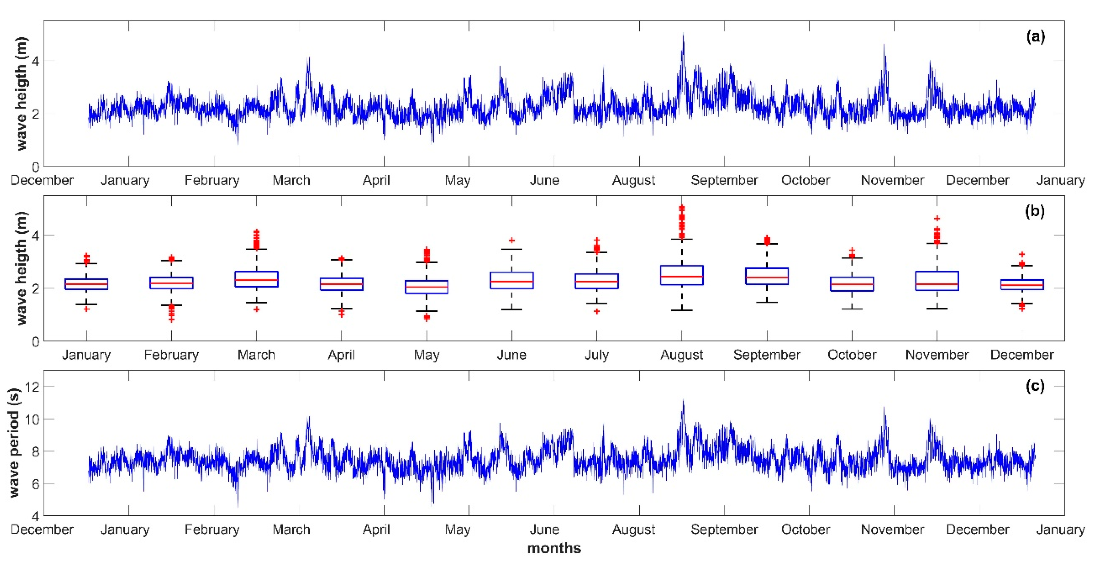
3. Results

Figure 4a shows the time series of the wave height for the point P1 of Figure 3, located at 73.25° W and 36.65° S (see Section 2.3). This series’ hourly annual mean is 2.5 m, with a standard deviation of 0.5 m (energy of 27.6 kW/m and 1.0 kW/m, respectively). While the annual median is 2.45 m (26.47 kW/m), and 75 and 25% are in the values 2.18 m (21 kW/m) and 2.79 (34 kW/m), respectively. The maximum height for the whole period was 4.96 m (11 August 2018), which corresponds to an energy of 108 kW/m.

The boxplot (Figure 4b) shows that the median varies with the seasons, having its maximum and minimum values in winter and summer, respectively. Summer presents less variability and with more stable values, with minima and maxima of 1.33 m (7.5 kW/m) and 3.54 m (55 kW/m), respectively. Simultaneously for this season, the percentiles show that 75% of summertime wave reaches heights greater than 2.1 m, corresponding to 20 kW/m. During winter, extreme values frequency increases to wave heights higher than 4 m (70 kW/m). The maxima and minima being 4.96 m (108 kW/m) and 1.04 m (5 kW/m), respectively. One can also note that, 75% of the time, it reaches values greater than 2.31 m (23 kW/m) during this season. The wave peak period (Figure 4c) has a mean of 7.8 s and presents its maximum and minimum values in winter and summer.

The amount of energy collected throughout the year for the most energetic sweep point (presented in Figure 1) is 270 MWh/m/year. The lowest as perceived by the radar is 160 MWh/m/year. Finally, a periodogram (not shown) showed amplitudes of the annual and semi-annual cycles being 0.2 and 0.1 m, respectively.

The HF radar raw data (before the outliers’ detection method was applied) is compared with the buoy (36.56° S–73.33° W) in Figure 5.

The buoy is quite far from the coast and is not precisely in a radar grid point. It is noticeable that, in that location (see Figure 3), the HF radar presents initially 50% fewer data than the buoy. In Figure 5, gaps are shown in both time series to demonstrate how damaging data loss can be. Thus, finally, our study only investigated grid cells where raw gaps do not exceed 40%. However, even if that place is out of the correct radar cover zone, although some extreme variation in the buoy data not captured in the HF radar, the main frequencies (semi-annual, seasonal) amplitudes agree remarkably. Figure 5b shows the time series of the period measured by radar and buoy. While the values show a similar trend, the magnitude of both does not match. Despite the previous mention, the buoy’s statistics are still equivalent to that of the chosen grid analyzed in the field. The annual mean is 2.26 m for radar and 2.12 m for buoy, with a standard deviation of 0.71 and 0.66 m, respectively. The index results for this grid cell are COV 0.9 for HF radar and 0.76 for buoy; SV is 0.1 for HF radar and 0.05 for buoy; MV is 0.16 for HF radar and 0.12 for the buoy. The mean wave power was also estimated, resulting from 23.8 kW/m for the radar data and 31.6 kW/ for the buoy. The normalized RMS is 0.27, and the normalized BIAS is 1.3.

The spatial analysis shows that the monthly averages shown in Figure 6 present a wave power variation between 10 and 40 kW per meter of the coast for the less and more energetic months. The maximum and minimum values, as expected, are obtained for the winter and summer months, respectively. In summer (December–February), the field values vary between 15 and 25 kW/m. The least energetic month is January, with a constant 20 kW/m. In winter (June–August), the values are between 20 and 40 KW/m, approximately twice as much as summer. August and September are the months in which more energy can be obtained, having values over 28 kW/m for approximately all the radar sweep.

Figure 7 shows both the annual accumulation and the coefficient of variation (COV, see Equation (5)) for the study area. The COV presents values between 0.3 and 0.5, with the highest values along the latitude 36.7°S, which coincides with one of the radar sweeps’ edges. In turn, the indices of seasonal and monthly variability were also calculated (see Equations (6) and (7)), which presented values between 0.06–0.4 and 0.1–0.6. The COV values are relatively small compared to the other indices (SV and MV), which indicates the wave field has a small variability, and the values are close to the average.

From the MV index analysis, it is clear that the values are higher than SV since the months compared (August and January) present significant differences, especially in the radar sweep’s central sector, where the energy presents its highest values.

In the location exemplified in Figure 4, the coefficients mentioned above obtained from the HF radar have the following values COV = 0.42, SV = 0.3, MV = 0.47. The site shows the highest wave power compared to the surrounding area and presents the highest variability indexes. Although wave power value assesses the location’s suitability, sites with constant energy flows are more attractive than those with high variability [31]. They are more reliable and allow constant energy injection into the power grid. The site selection must combine both characteristics, high power with low variability.

4. Discussion and Conclusions

Chile’s energy goals are clear; by 2050, 70% of the national energy matrix must be covered by renewable energy [39]. According to reports [40] on energy projects under construction, most of them are wind and solar energy since northern Chile has one of the highest solar radiation levels. On the other hand, wind energy has sectors south of the country where the potential is quite favorable. However, due to the long Chilean coastline, wave energy is also considered a potential source to supply the energy demand [41,42]. Notably, the work of [26,43,44,45,46] has already estimated the potential using numerical models compared to buoys and satellites. However, when it comes to obtaining information in high spatial resolution, there is no comparable method. It is the main reason for our study.

As mentioned throughout this paper, the advantage of HF radars is that they can provide high spatial and temporal resolution with scales from 0.3 to 50 km and a minimum of 30 min, respectively [12,23,47,48]. Additionally, they allow for sweeping a large area of the ocean. Being remote instruments, they are not affected by the hostile state that it can present. Therefore, despite some inaccuracies that HF radars can present [19], this study is valuable to understand their usefulness. In addition, the measurement they provide is also a resource to validate and complement information from other sources.

We worked with an HF radar to obtain the wave power fields of approximately 800 km² in front of Concepción. The treated data’s spatial resolution is 2 km, and temporal resolution is 1 h, from December 2017 to January 2019. It is necessary to highlight that a one-year period is not long enough to understand the wavefield, limiting the work thoroughly. However, it can be significant if used as a complement for other observations, either remote or in situ, to understand the area’s wave climate.

As the first interest of the installation of HF radars by CHIOOS was the detection of a tsunami, for the moment, this work only uses data from a single radar. While single radar estimates of significant wave height do not provide as accurate a measurement as dual radars, let us note that under homogeneous wave conditions, individual radars have a slight advantage over a conventional buoy [19]. Similarly, the local values collected from the radar were close to those found in other works [24,25,35].

The HF radar data were contrasted with in-situ data (buoy). However, given the buoy location at 36.56°S 73.33°W, where the HF radar’s temporal coverage is less than 50%, it provides very low representativeness. Nevertheless, the buoy’s statistics are still equivalent to that of the chosen grid analyzed in the field. The annual mean is 2.26 m for radar and 2.12 m for buoy, with a standard deviation of 0.71 m and 0.66 m. The annual and semi-annual cycles were compared with data from a wave-atlas produced by Universidad de Valparaiso [35] through numerical models (WW3). Thus, although the wave-atlas epoch (1980–2015) does not coincide with ours, the results show similar annual and semi-annual cycle characteristics; 0.25 m and 0.11 m for the radar, the atlas showing 0.3 m and 0.1 m, respectively.

The potential annual mean average power is 23 kW/m. However, this value depends on the used peak period. For the peak period, as mentioned in Section 2.2.2, we used one obtained from the official bibliography; the Chilean marine atlas [35,49]. However, while we could have used the buoy peak period instead, the variations of these appear relatively discretized (see Figure 5b), showing a considerable variability around 12.4 s. The majority of works investigated, including the atlas, showed values around 10 s without presenting many variations throughout the year. In addition, the comparison between the radar and buoy period data series also shown in Figure 5b reveals, due to the absence of data of the radar sweep around this location, the lack of correlation between what the buoy measures and what the radar provides there. It is also interesting to know how much the final energy would have varied if we had taken one period value or the other; HF radar’s or the buoy’s. The average mean peak period for the entire radar sweep (not shown) is 7.48 s with a standard deviation of 0.19 but varies between 7.1 and 7.9 s over the entire zone, which is less than 1 s, decreasing while approaching the coast. The radar mean peak period closest to the buoy is 7.6 s, with a standard deviation of 0.7 s (Figure 5b). The buoy mean peak period, calculated only for the overlapping radar times, is 12.4 s with a standard deviation of 2.6 s (Figure 5b). Using the buoy data as reality, assuming that the radar nearest grid is correct, we computed a calibrated period gridded field. Thus, using the calibrated mean peak period the wave mean power in that location would have increased by 20%, 4.6 kW/m. On the contrary, having used the radar’s mean peak period, 24% less, that is 4.4 kW/m.

Nevertheless, the potential annual average powers fluctuate between 15 and 30 kW/m, depending on the sector within the sweep. As stated in [50], approximately 20 kW/m will make wave energy economically viable. As wave energy is not as mature as other renewable energies (like solar or wind), the economic viability not only depends on the amount of power a location can provide. The cost of the WECs is an essential part of the cost of a wave farm. The cost of operation and maintenance is also high, as corresponds to a facility in the sea [51]. The maximum power occurs during the winter season at 73.25 W and 36.65 S, approximately 15 km from the coast. The seasonal average is 37 kW/m, corresponding to a wave height of approximately 2.9 m, with a standard deviation of 1.6 kW/m. The maximum height at this point was 4.96 m (108 kW/m). In summer (December-February), the values vary between 15 and 25 kW/m. The least energetic month is January, presenting a constant 20 kW/m, half the one obtained in winter. One can note that throughout the year, 75% of the time, the wave height is above 2.2 m, which means that 75% of the time, the power will be a minimum of 22 kW/m. If this is carried out in terms of energy, it corresponds to a minimum of 193 MWh/m/year.

The SV and MV indices calculated presented values between 0.06–0.4 and 0.1–0.6, similar to those presented by [26]. These indices are relatively low compared to other studies that present similar potential magnitudes, such as [31,52]. Additionally, as mentioned before, the site selection must consider the wave power and variability of the area; here, the COV presents a lower variability than the considerable wave potential found. As a whole, the different indices make the area a more than convenient place for energy extraction.

We investigated the energy consumption of the areas close by. On average, a household consumes approximately 200 kWh per month, presenting a maximum peak in winter with values close to 230 kWh/month and a minimum in summer of 150 kWh/month [53]. Our work shows that this value is less than what can be extracted from a single grid cell, which is 2 × 2 km, since 75% of the time, the energy extracted would be larger than 16.6 MWh/month. Annually the maximum that could be collected is 270 MWh/m/year, and the lowest as perceived by the radar is 160 MWh/m/year. Considering a simple device, for example, an OWC with an efficiency of 40% [54,55], a single wave energy collector could have an approximate annual savings of USD 13,500, which would supply the average annual energy demand of approximately 33 houses, equivalent to avoiding 32.31 tonCO2eq/year [56]. The most significant advantage of wave energy is its high-power density, meaning that it can harness more energy than other renewable energies. Due to the novelty and newness of wave energy converters, it is impossible to provide a specific number of devices that can attain powers as big as wind or solar energy. For example, Ref. [51] shows several devices’ performance, and the installed power varies between 6 kW and 15 MW. Thus, to reach 1 GW of installed power, the quantity of WEC can vary between 160,000 and 66. Likewise, the amount of area used to display the WECs also will change. Noteworthy, there are so many WECs types and locations where this can be installed that each case has to be evaluated case by case. Let us note something interesting to consider; hybrid systems, coupling waves and wind energy in the same facility [57]. It will provide an even more stable supply using the same area.

This work made it possible to estimate the wave power in front of the Biobío region, determining the area’s suitability for its low variability and high energy concentration. With the high-resolution information provided by the HF radar, the best location for energy extraction can be identified. The utility of HF radars in energy terms relies on its high resolution, both temporal and spatial, given the ability to compare locations of interest within the same area. The possibility to implement a transportable radar to measure the high frequencies waves rank this instrument as an excellent asset to establish the wave power of a location.

As established throughout this work, even when a single radar can provide wave information, it can present ambiguities. This cannot be solved using only the radar’s information. Of course, eventually, two radar systems would be ideal. However, not being cheap systems, we must enhance what we already have. Thus, one of our research’s next stages could be to move the transportable HF radar close to the buoy to calibrate it correctly. Instead, we can use coastal video imagery for doing so [58,59]. We should also investigate an up-and-coming smartphone-based camera system recently assessed for coastal image classification [60].

Another great applicability of an HF marine radar system is its complementary use to satellite measurements or numerical models. In turn, radar data can be a valuable tool for the calibration of satellite data such as CFOSAT [61] and SWOT [62]. For example, SWOT’s main objective is to measure ocean topography with centimeter-scale accuracy over kilometer-scale spatial resolution [63]. Therefore, HF radar measurements that also have a high resolution can be an accurate validation system. It shows the usefulness of HF marine radar as an instrument of remote sensing to study wave patterns and wave energy potential of vast areas at a high resolution.

References

- Cornett, A. A Global Wave Energy Resource Assessment. In Proceedings of the Eighteenth International Offshore and Polar Conference, Vancouver, BC, Canada, 6–11 July 2008. [Google Scholar]
- Arinaga, R.A.; Cheung, K.F. Atlas of global wave energy from 10 years of reanalysis and hindcast data. Renew. Energy 2012, 39, 49–64. [Google Scholar] [CrossRef]
- Reeve, D.E.; Chen, Y.; Pan, S.; Magar, V.; Simmonds, D.J.; Zacharioudaki, A. An investigation of the impacts of climate change on wave energy generation: The Wave Hub, Cornwall, UK. Renew. Energy 2011, 36, 2404–2413. [Google Scholar] [CrossRef] [Green Version]
- Gunn, K.; Stock-Williams, C. Quantifying the global wave power resource. Renew. Energy 2012, 44, 296–304. [Google Scholar] [CrossRef]
- Mork, G.; Barstow, S.; Kabuth, A.; Pontes, M.T. Assessing the Global Wave Energy Potential. In Proceedings of the 29th International Conference on Ocean, Offsh-ore and Arctic Engineering, Shanghai, China, 6–11 June 2010; Volume 3, pp. 447–454. [Google Scholar]
- European Commission. Technology Information: Ocean Energy; European Commission: Brussels, Belgium, 2014. [Google Scholar]
- IRENA. Renewable Capacity Statistics 2017; International Renewable Energy Agency (IRENA): Abu Dhabi, UAE, 2017. [Google Scholar]
- Europe Ocean Energy. 2030 Ocean Energy Vision; Europe Ocean Energy: Brussels, Belgium, 2019. [Google Scholar]
- Trowbridge, J.; Weller, R.; Kelley, D.; Dever, E.; Plueddemann, A.; Barth, J.A.; Kawka, O. The Ocean Observatories Initiative. Front. Mar. Sci. 2019, 6. [Google Scholar] [CrossRef]
- Lillesand, T.; Kiefer, R.; Chipman, J. Remote Sensing and Image Interpretation, 7th ed.; Wiley: Hoboken, NJ, USA, 2015. [Google Scholar]
- Ribal, A.; Young, I.R. 33 years of globally calibrated wave height and wind speed data based on altimeter observations. Sci. Data 2019, 6. [Google Scholar] [CrossRef] [Green Version]
- Gurgel, K.W.; Antonischiki, G. Remote Sensing of Surface Currents and Waves by the Hf Radar Wera. In Proceedings of the International Conference on Electronic Engineering in Oceanography, Southampton, UK, 23–25 June 1997. [Google Scholar]
- Essen, H.H.; Gurgel, K.W.; Schlick, T. Measurement of ocean surface waves by HF radars using a direction finding receive antenna. In Proceedings of the IGARSS 2000. IEEE 2000 International Geoscience and Remote Sensing Symposium. Taking the Pulse of the Planet: The Role of Remote Sensing in Managing the Environment. Proceedings (Cat. No.00CH37120), Honolulu, HI, USA, 24–28 July 2000. [Google Scholar]
- Lipa, B.; Barrick, D.; Broug, J.; Nyden, B. HF Radar Detection of Tsunamis. J. Oceanogr. 2006, 62, 705–716. [Google Scholar] [CrossRef]
- Lopez, G.; Conley, D.C. Comparison of HF Radar Fields of Directional Wave Spectra Against In Situ Measurements at Multiple Locations. J. Mar. Sci. Eng. 2019, 7, 271. [Google Scholar] [CrossRef] [Green Version]
- Saviano, S.; Kalampokis, A.; Zambianchi, E.; Uttieri, M. A year-long assessment of wave measurements retrieved from an HF radar network in the Gulf of Naples (Tyrrhenian Sea, Western Mediterranean Sea). J. Oper. Oceanogr. 2019, 12, 1–15. [Google Scholar] [CrossRef]
- Helzel, T.; Lopez, O.; Wyatt, L.R. Ocean Radar for the Planning and Operational Phase of Off-Shore Renewable Energy System; IEEE: Piscataway, NJ, USA, 2011. [Google Scholar]
- Patel, R.P.; Nagababu, G.; Kumar, S.V.A.; Seemanth, M.; Kachhwaha, S.S. Wave resource assessment and wave energy exploitation along the Indian coast. Ocean Eng. 2020, 217, 107834. [Google Scholar] [CrossRef]
- Wyatt, L.R. An evaluation of wave parameters measured using a single HF radar system. Can. J. Remote Sens. 2002, 28, 205–218. [Google Scholar] [CrossRef]
- Wyatt, L.R. Significant waveheight measurement with h.f. radar. Int. J. Remote Sens. 1988, 9, 1087–1095. [Google Scholar] [CrossRef]
- Heron, M.L.; Atwater, D.P. Temporal and spatial resolution of HF ocean radars. Ocean Sci. J. 2013, 48, 99–103. [Google Scholar] [CrossRef]
- Fujii, S.; Heron, M.L.; Kim, K.; Lai, J.-W.; Lee, S.-H.; Wu, X.; Wu, X.; Wyatt, L.R.; Yang, W.-C. An overview of developments and applications of oceanographic radar networks in Asia and Oceania countries. Ocean Sci. J. 2013, 48, 69–97. [Google Scholar] [CrossRef]
- Roarty, H.; Cook, T.; Hazard, L.; George, D.; Harlan, J.; Cosoli, S.; Wyatt, L.; Alvarez Fanjul, E.; Terrill, E.; Otero, M.; et al. The Global High Frequency Radar Network. Front. Mar. Sci. 2019, 6. [Google Scholar] [CrossRef]
- Young, I.R. Seasonal Variability Of The Global Ocean Wind And Wave Climate. Int. J. Climatol. 1999, 19, 931–950. [Google Scholar] [CrossRef]
- Aguirre, C.; Rutllant, J.A.; Falvey, M. Wind waves climatology of the Southeast Pacific Ocean. Int. J. Climatol. 2017, 37, 4288–4301. [Google Scholar] [CrossRef]
- Lucero, F.; Catalán, P.A.; Ossandón, Á.; Beyá, J.; Puelma, A.; Zamorano, L. Wave energy assessment in the central-south coast of Chile. Renew. Energy 2017, 114, 120–131. [Google Scholar] [CrossRef]
- Leys, C.; Ley, C.; Klein, O.; Bernard, P.; Licata, L. Detecting outliers: Do not use standard deviation around the mean, use absolute deviation around the median. J. Exp. Soc. Psychol. 2013, 49, 764–766. [Google Scholar] [CrossRef] [Green Version]
- Amidror, I. Scattered data interpolation methods for electronic imaging systems: A survey. J. Electron. Imaging 2002, 11. [Google Scholar] [CrossRef]
- Liepins, V. An algorithm for evaluating a discrete Fourier transform for incomplete data. Autom. Control Comput. Sci. 1996, 30, 20–29. [Google Scholar]
- Liepins, V. Extended Fourier analysis of signals. arXiv 2013, arXiv:1303.2033. [Google Scholar]
- Bingölbali, B.; Jafali, H.; Akpınar, A.; Bekiroğlu, S. Wave energy potential and variability for the south west coasts of the Black Sea: The WEB-based wave energy atlas. Renew. Energy 2020, 154, 136–150. [Google Scholar] [CrossRef]
- Holthuijsen, L.H. Waves in Oceanic and Coastal Waters; Cambridge University Press: Cambridge, UK, 2007; Volume 1. [Google Scholar]
- Soares, C.G. (Ed.) Advances in Renewable Energies Offshore; Taylor & Francis: London, UK, 2018. [Google Scholar]
- Ingram, D.M.; Smith, G.; Bittencourt Ferreira, C.; Smith, H. Protocols for the Equitable Assessment of Marine Energy Converters; The Institute for Energy Systems: Edinburgh, UK, 2011. [Google Scholar]
- Beyá, J.; Álvarez, M.; Gallardo, A.; Hidalgo, H.; Aguirre, C.; Valdivia, J.; Parra, C.; Méndez, L.; Contreras, F.; Winckler, P.; et al. Atlas de Oleaje de Chile; Escuela de Ingeniería Civil Oceánica—Universidad de Valparaiso: Valparaiso, Chile, 2016. [Google Scholar]
- Reguero, B.G.; Losada, I.J.; Méndez, F.J. A global wave power resource and its seasonal, interannual and long-term variability. Appl. Energy 2015, 148, 366–380. [Google Scholar] [CrossRef]
- Silva, D.; Martinho, P.; Guedes Soares, C. Wave energy distribution along the Portuguese continental coast based on a thirty three years hindcast. Renew. Energy 2018, 127, 1064–1075. [Google Scholar] [CrossRef]
- Alizadeh, M.J.; Alinejad-Tabrizi, T.; Kavianpour, M.R.; Shamshirband, S. Projection of spatiotemporal variability of wave power in the Persian Gulf by the end of 21st century: GCM and CORDEX ensemble. J. Clean. Prod. 2020, 256, 120400. [Google Scholar] [CrossRef]
- de Energía, C.C. Energía 2050, Política Energética de Chile; Ministerio de Energía: Santiago, Chile, 2017. [Google Scholar]
- Comisión Nacional de Energía. Anuario Estadístico de Energía; Ministerio de Energía: Santiago, Chile, 2018; pp. 1–162. [Google Scholar]
- Villavicencio, P. Chile Cuenta Con Nuevo Centro de Investigación, Pionero en Energía Marina. Available online: https://www.elciudadano.com/ciencia-tecnologia/centro-de-energia-marina/06/18/ (accessed on 10 September 2020).
- MERIC. Ministro de Energía Inaugura Pionero Centro de Investigación en Energía Marina. Available online: https://www.meric.cl/en/ministro-de-energia-inaugura-pionero-centro-de-investigacion-en-energia-marina-2/ (accessed on 10 September 2020).
- Mediavilla, D.G.; Figueroa, D. Assessment, sources and predictability of the swell wave power arriving to Chile. Renew. Energy 2017, 114, 108–119. [Google Scholar] [CrossRef]
- Mediavilla, D.G.; Sepúlveda, H.H. Nearshore assessment of wave energy resources in central Chile (2009–2010). Renew. Energy 2016, 90, 136–144. [Google Scholar] [CrossRef]
- Mazzaretto, O.M.; Lucero, F.; Besio, G.; Cienfuegos, R. Perspectives for harnessing the energetic persistent high swells reaching the coast of Chile. Renew. Energy 2020, 159, 494–505. [Google Scholar] [CrossRef]
- Monárdez, P.; Acuña, H.; Scott, D. Evaluation of the Potential of Wave Energy in Chile. In Proceedings of the ASME 2008 27th International Conference on Offshore Mechanics and Arctic Engineering, Estoril, Portugal, 15–20 June 2008; Volume 6, pp. 801–809. [Google Scholar]
- Wyatt, L.R. Wave and Tidal Power measurement using HF radar. IMEJ 2018, 1. [Google Scholar] [CrossRef]
- Wyatt, L.R. High frequency radar applications in coastal monitoring, planning and engineering. Aust. J. Civ. Eng. 2014, 12, 1–15. [Google Scholar] [CrossRef]
- Beyá, J.; Álvarez, M.; Gallardo, A.; Hidalgo, H.; Winckler, P. Generation and validation of the Chilean Wave Atlas database. Ocean Model. 2017, 116, 16–32. [Google Scholar] [CrossRef]
- Sandberg, A.; Klementsen, E.; Muller, G.; de Andres, A.; Maillet, J. Critical Factors Influencing Viability of Wave Energy Converters in Off-Grid Luxury Resorts and Small Utilities. Sustainability 2016, 8, 1274. [Google Scholar] [CrossRef] [Green Version]
- Astariz, S.; Iglesias, G. The economics of wave energy: A review. Renew. Sustain. Energy Rev. 2015, 45, 397–408. [Google Scholar] [CrossRef]
- Amrutha, M.M.; Sanil Kumar, V. Spatial and temporal variations of wave energy in the nearshore waters of the central west coast of India. Ann. Geophys. 2016, 34, 1197–1208. [Google Scholar] [CrossRef] [Green Version]
- Comisión Nacional de Energía. Consumo Eléctrico Anual por Comuna y Tipo de Cliente; Energía Abierta; Comisión Nacional de Energía: Santiago, Chile, 2019. [Google Scholar]
- Aderinto, T.; Li, H. Review on Power Performance and Efficiency of Wave Energy Converters. Energies 2019, 12, 4329. [Google Scholar] [CrossRef] [Green Version]
- Maldonado, C. Stochastic Modelling of Owc Device and Power Production; Pontificia Universidad Catolica De Chile: Santiago, Chile, 2017. [Google Scholar]
- Comisión Nacional de Energía. Factor de Emisión, Promedio Anual; Energía Abierta; Comisión Nacional de Energía: Santiago, Chile, 2019. [Google Scholar]
- Astariz, S.; Iglesias, G. Co-located wind and wave energy farms: Uniformly distributed arrays. Energy 2016, 113, 497–508. [Google Scholar] [CrossRef] [Green Version]
- Cienfuegos, R.; Villagran, M.; Aguilera, J.C.; Catalán, P.; Castelle, B.; Almar, R. Video monitoring and field measurements of a rapidly evolving coastal system: The river mouth and sand spit of the Mataquito River in Chile. J. Coast. Res. 2014, 70, 639–644. [Google Scholar] [CrossRef]
- Cang, Y.; He, H.; Qiao, Y. Measuring the Wave Height Based on Binocular Cameras. Sensors 2019, 19, 1338. [Google Scholar] [CrossRef] [Green Version]
- Valentini, N.; Balouin, Y. Assessment of a Smartphone-Based Camera System for Coastal Image Segmentation and Sargassum monitoring. J. Mar. Sci. Eng. 2020, 8, 23. [Google Scholar] [CrossRef] [Green Version]
- Hauser, D.; Tourain, C.; Lachiver, J.M. CFOSAT: A New Mission in Orbit to Observe Simultaneously Wind and Waves at the Ocean Surface. Space Res. Today 2019, 206, 15–21. [Google Scholar] [CrossRef]
- Aouf, L.; Hauser, D.; Dalphinet, A.; Giordani, H. SWOT-Waves: For the Improvement of Operational Wave Forecasting; NASA: Washington, DC, USA, 2020.
- Peral, E.; Rodríguez, E.; Esteban-Fernández, D. Impact of Surface Waves on SWOT’s Projected Ocean Accuracy. Remote Sens. 2015, 7, 14509–14529. [Google Scholar] [CrossRef] [Green Version]
Publisher’s Note: MDPI stays neutral with regard to jurisdictional claims in published maps and institutional affiliations. |
© 2021 by the authors. Licensee MDPI, Basel, Switzerland. This article is an open access article distributed under the terms and conditions of the Creative Commons Attribution (CC BY) license (http://creativecommons.org/licenses/by/4.0/).
Share and Cite
Mundaca-Moraga, V.; Abarca-del-Rio, R.; Figueroa, D.; Morales, J. A Preliminary Study of Wave Energy Resource Using an HF Marine Radar, Application to an Eastern Southern Pacific Location: Advantages and Opportunities. Remote Sens. 2021, 13, 203. https://doi.org/10.3390/rs13020203
Mundaca-Moraga V, Abarca-del-Rio R, Figueroa D, Morales J. A Preliminary Study of Wave Energy Resource Using an HF Marine Radar, Application to an Eastern Southern Pacific Location: Advantages and Opportunities. Remote Sensing. 2021; 13(2):203. https://doi.org/10.3390/rs13020203
Chicago/Turabian StyleMundaca-Moraga, Valeria, Rodrigo Abarca-del-Rio, Dante Figueroa, and James Morales. 2021. "A Preliminary Study of Wave Energy Resource Using an HF Marine Radar, Application to an Eastern Southern Pacific Location: Advantages and Opportunities" Remote Sensing 13, no. 2: 203. https://doi.org/10.3390/rs13020203