Satellite Based Fraction of Absorbed Photosynthetically Active Radiation Is Congruent with Plant Diversity in India

Abstract

A dynamic habitat index (DHI) based on satellite derived biophysical proxy (fraction of absorbed photosynthetically active radiation, FAPAR) was used to evaluate the vegetation greenness pattern across deserts to alpine ecosystems in India that account to different biodiversity. The cumulative (DHI-cum), minimum (DHI-min), and seasonal (DHI-sea) DHI were generated using Moderate Resolution Imaging Spectroradiometer (MODIS)-based FAPAR. The higher DHI-cum and DHI-min represented the biodiversity hotspots of India, whereas the DHI-sea was higher in the semi-arid, the Gangetic plain, and the Deccan peninsula. The arid and the trans-Himalaya are dominated with grassland or barren land exhibit very high DHI-sea. The inter-year correlation demonstrated an increase in vegetation greenness in the semi-arid region, and continuous reduction in greenness in the Northeastern region. The DHI components validated using field-measured plant richness data from four biogeographic regions (semi-arid, eastern Ghats, the Western Ghats, and Northeast) demonstrated good congruence. DHI-cum that represents the annual greenness strongly correlated with the plant richness (R² = 0.90, p-value < 0.001), thereby emerging as a suitable indicator for assessing plant richness in large-scale biogeographic studies. Overall, the FAPAR-based DHI components across Indian biogeographic regions provided understanding of natural variability of the greenness pattern and its congruence with plant diversity.

1. Introduction

Biodiversity has a powerful influence on ecosystem dynamics and functions at various geographical scales [1,2]. Global biodiversity observations are needed to provide a better understanding of the distribution of biodiversity, to better identify high priority areas for conservation, and to maintain essential ecosystem goods and services [3]. The gradual decline in biodiversity endangers essential ecosystem services and risks unacceptable environmental consequences [4]. The traditional in situ biodiversity monitoring practice is insufficient to solve the problems associated with biodiversity conservation [5].

Remote sensing technology has provided an effective and evident way to address biodiversity patterns at different geographical scales [6]. Space-borne platforms operate different earth observation satellites, which presents the potential to prepare conservation responses that are commensurate with the scale of conservation [7]. Satellite sensors measure the reflected solar energy emitted from the ground that determines the radiation-interception characteristics of plant canopies linked to photosynthesis [8]. The difference between the carbon assimilated by plant leaves during photosynthesis is a quantitative measure of plant growth and carbon uptake, which represents the vegetation productivity [9,10]. Due to dynamic environmental conditions, vegetation productivity varies with time and space [11,12].

Satellite-derived biophysical proxies provide clues about diversity patterns as they are used for productivity estimation and quantification of spatial heterogeneity of vegetation [13]. Plant richness is a straight forward indicator of plant diversity, which is directly associated with habitat heterogeneity [14,15]. Forest type and species composition plays a vital role to correlate between satellite-derived biophysical proxy and plant richness [16]. Comparison of temporal scales exhibit that the annual pattern of correlation faired more than seasonal (i.e., monsoon) between satellite-derived biophysical proxy and plant richness in the Western Ghats, India [17]. Chitale et al. [18] obtained a high correlation between satellite-derived biophysical proxies and plant richness for open canopy vegetation classes with low species richness (grasslands, scrubs, and dry deciduous forests) followed by vegetation classes with moderately dense canopy in the Western Ghats, Indo-Burma and Himalayan regions in India.

Satellite observations have captured an increase in vegetation growth and productivity mostly in Asia, Africa, and Europe due to agricultural intensification and other human activities [19,20,21]. In India, the vegetation greenness has increased much more due to agriculture (82%) compared with forests (4.4%) [22]. Also, it has been reported that the crop production has improved up to six times in the past five decades [23]. Agricultural intensification has increased the vegetation greenness in the Western Himalaya, while reduced pre-monsoon moisture levels has resulted a decrease in the greenness pattern in the eastern Himalaya [24]. A study analyzed the seasonal NDVI trend from 2000 to 2014, which reported greening-up due to the rain-fed cultivated area in the lower elevation, while browning-up trend has been consistent along the elevational range that holds closed needle-leaved forests and alpine scrublands in the Uttarakhand Himalaya [25]. A reduction in vegetation greenness with warmer temperatures was reported for trans-Himalayan and western Indian regions [26,27]. Chakraborty et al. [28] analyzed seasonal greenness trends in different forest types of India and found changes in protected areas across India (Simlipal Wildlife Sanctuary, Rajaji National Park, Achanakmar Wildlife Sanctuary, Sundarbans Biosphere Reserve).

The satellite proxies (fraction of absorbed photosynthetically active radiation (FAPAR), leaf area index (LAI), etc.) derived using multiple bands have been found to be better estimators compared to other satellite-derived biophysical proxies (normalized difference vegetation index—NDVI, enhanced vegetation index—EVI, etc.) of habitat conditions and therefore used to explain greenness [29]. The dynamic habitat index (DHI) based on satellite-derived biophysical proxies has been found to provide a good approximation of the habitat conditions [30,31]. The DHI has three components, and each of these is relevant to an hypothesis: (1) DHI-cumulative (DHI-cum) is used to evaluate the available energy hypothesis, according to which greater energy availability is associated with higher productivity and hence with greater biodiversity [32,33,34]. (2) DHI-minimum (DHI-min) is a proxy for the environmental stress hypothesis, according to which the biodiversity is greater where there is a higher minimum productivity throughout the year [35,36,37]. (3) DHI-seasonal (DHI-sea) is used to evaluate the environmental stability hypothesis, according to which the biodiversity is greater where the intra-annual variability in productivity is lower [38]. The Moderate Resolution Imaging Spectroradiometer (MODIS) sensor has been used widely to derive the DHI components that are of significance in explaining biodiversity. MODIS-FAPAR data have been used to calculate the DHI to evaluate the relationships between habitat heterogeneity and faunal diversity in the Canadian province of Ontario, United States and Australia [30,39,40]. FAPAR DHI-min characterized 70% of the arid region of the Australian continent as having low greenness cover [41]. Areas under agricultural crops had moderate annual FAPAR levels, large variations in greenness and low annual minimum cover. With increasing annual FAPAR, the greenness cover and the plant diversity increased [42]. In contrast, high annual FAPAR was found in the Western Ghats with low annual variation [17]. Further, the DHI can be integrated with the basic ecological drivers, i.e., environmental heterogeneity (climatic, geophysical variables), habitat productivity, and land cover change, to map and monitor changes in biodiversity [43,44]. However, DHI-min and DHI-sea represented the climatic and anthropogenic induced changes, hence can be useful in addressing land degradation and development [4].

Though the remote sensing proxy-derived DHI explains vegetation productivity ranges and greenness patterns, the validation and pattern analysis need to be performed using sampled plant data. A dynamic habitat index (DHI) based on a satellite derived biophysical proxy (fraction of absorbed photosynthetically active radiation, FAPAR) was used to evaluate the vegetation greenness pattern across deserts to alpine ecosystems in India. Further, the cumulative (DHI-cum), seasonal (DHI-sea), and minimum (DHI-min) DHI were used to establish correlation with biodiversity in varied biogeographic regions of India during 2001–2015. This study outcome would demonstrate the variability in greenness cover across the Indian biogeographic regions, providing valuable insights towards the conservation and management plan.

2. Materials and Methods

2.1. Study Area

The entire Indian nation that consists of the mainland with islands on either side, i.e., the Andaman & Nicobar Islands (in the east) and the Lakshadweep Islands (in the west) was selected as the study area. The Indian mainland has the largest peninsula, extending 3219 km from north to south and 2977 km from east to west, with a geographic extent of 3,287,263 km² [45]. Across the 10 biogeographic regions (Figure 1a), India accommodates a wide range of vegetation with grassland and pastureland in arid and semi-arid regions to the broadleaved and alpine forest in Himalaya and Northeast regions. The climatic profile varies from temperate in the north to monsoonal in the south with large variation in precipitation pattern across its length and breadth. The country accommodates diverse topography, soil, and climate.

2.2. Satellite Data

National Aeronautics and Space Administration (NASA) launched the TERRA (1999) and AQUA (2001) satellites, which aboard the MODIS sensors for global carbon cycle monitoring [46]. The MODIS instruments have 36 spectral bands (0.4 μm to 14.4 μm) at varying spatial resolutions (2 bands at 250 m, 5 bands at 500 m, and 29 bands at 1 km) [47]. NASA provides a suite of atmospherically, geo-registered, data products of MODIS on a routine basis, including FAPAR [48]. The geo-rectified and atmospherically corrected MODIS-FAPAR (MOD15A2H) data were downloaded for the period of 2001–2015 (https://earthdata.nasa.gov/), with spatial resolution of 500 m and temporal resolution of 8 days. All the image-processing tasks such as mosaicking, projections, masking, and normalization were performed using the MRT and ArcGIS (10.5 version) tools, and the temporal resolution was brought to a monthly time frame.

2.3. Generation of DHI Components and Their Composite

Monthly maximum of MODIS FAPAR values was the basic input data set to compute the three relevant annual indices for the DHI analysis. DHI-cum that represents the cumulative annual productivity of a year, was derived as the arithmetic summation of the monthly FAPAR data and the index vary from 0 to 12 [49]. DHI-min that represents the lowest monthly productivity in a year was derived as the arithmetic minima of the monthly FAPAR data and the index varies from 0 to 1. Similarly, DHI-sea that represents the seasonal variability in greenness, was computed by dividing the standard deviation and mean of the monthly FAPAR data for a year and the index vary from −∞ to +∞ [49]. A DHI composite image was derived by assigning DHI-cum, DHI-min and DHI-sea to green, blue, red color plains respectively for visualization and indication on the greenness cover and productivity. Further, the inter-annual variability (2001–2015) of the three DHI components were adjudged by estimating the correlation, regression and standard deviation [4].

Correlation coefficient:

$$\frac{\sum \left(x-\overline{x}\right) \left(y-\overline{y}\right)}{\sqrt{\sum {\left((x-\overline{x}\right)}^2} \sqrt{\sum {\left(y-\overline{y}\right)}^2}}$$

(1)

where x represents number of year and y represents the pixel values corresponding to DHI components (DHI-cum or DHI-min or DHI-sea).

Regression coefficient:

$$\frac{ \mathrm{N}\times {{\displaystyle \sum }}_{n=1}^N\mathrm{n} \times {DHI}_{\mathrm{i}} - ({{\displaystyle \sum }}_{n=1}^{N}n) ({{\displaystyle \sum }}_{n=1}^N{DHI}_{\mathrm{i}})}{(\mathrm{N}\times {{\displaystyle \sum }}_{n=1}^N{n}^2 - ({{{\displaystyle \sum }}_{n=1}^{N}n)}^2)}$$

(2)

where N and n represents the total number of years and individual year from 2001 to 2015, respectively and DHI_i represents the pixel values correspond to DHI-cum or DHI-min or DHI-sea.

Standard deviation (SD):

$$\frac{\sqrt{\sum {\left(DH{I}_{\mathrm{i}}-\mathrm{\mu }\right)}^2}}{N}$$

(3)

where DHI_i represents the yearly pixel values correspond to DHI-cum or DHI-min or DHI-sea, µ represents the mean of those pixel values from 2001 to 2015, and N represents the total number of years evaluated.

2.4. DHI Components and Plant Richness

The plant data for the study sites was procured from a national project entitled ‘Biodiversity Characterization at Landscape Level (BCLL)’ that was carried out during 1997–2012 [50]. The stratified random sampling was considered to lay nested quadrats of size 20 × 20 m² for trees (>15 cm, circumference at breast height-cbh) and lianas, two 5 × 5 m² plots for shrubs and saplings (>5 cm and <10 cm cbh), and four 1 × 1 m² plots for herbs and seedlings. The database has a record of 15,656 geo-tagged field plots and 6222 unique species from 10 biogeographic regions of India.

Four biogeographic regions (semi-arid, eastern Ghats, Western Ghats, and Northeast) having varied moisture level, plant richness and environmental heterogeneity were chosen for analysis of pattern between the plant richness and the DHI components. These regions encompass 7365 geo-tagged nested quadrats from the BCLL database. The unique species count from each nested quadrat represented the plant richness for the respective quadrat. The pixel values of averaged DHI components were linked using corresponding plant richness data from 7365 nested quadrat locations for the four biogeographic regions using ArcGIS platform [51]. Firstly, the yearly variations in DHIs from 2001 to 2015 in the four biogeographic regions were visualized using 3-D scatter plots. It was generated by utilizing the mean of each DHI components for each year that calculated the Euclidean distance for the selected biogeographic regions of India. Secondly, the distribution of plant richness from 7365 quadrats were plotted in box diagram along the average of DHIs. In the box plot, mean values denote the level of accuracy, whereas R² and p-values indicate the significance of the plant richness distribution for each DHI component. The standard deviation of three DHI components were randomly chosen to demonstrate the variation in greenness cover at a test site (93.84°E, 27.49°N) in the Northeastern region.

3. Results

3.1. Visualizing Greenness Pattern Using DHI Components along Indian Biogeographic Regions

The DHI-cum that represents the annual cumulative greenness, varied from 4 to 8, 2 to 8, and 2 to 6 along the western Himalaya, eastern Ghats, and the Gangetic plain regions respectively, during 2001–2015 (Figure 2). However, the DHI-cum range was less for the semi-arid and Deccan peninsula (0 to 4), and more for the Himalayan (0 to 11), Northeast (0 to 11), and Western Ghats (2 to 11) regions. Interestingly, the eastern part of the Deccan peninsula demonstrated DHI-cum variation between 0 to 6 and 0 to 12 in alternate years during 2001–2015 (Figure 2). The grasslands or scrublands on very fertile lands across the riverbeds demonstrated annual greenness of 2 to 6, which are mostly seasonal contributions. The DHI-cum reflected between 0 and 2 for non-vegetated classes as snow cover, rivers, and deserts. Thus, Indian heterogeneous biogeographic regions clearly demonstrated DHI-cum variation between 0 and 12 with varied greenness.

The DHI-min exhibits the status for minimum greenness sustained throughout a particular year. The DHI-min ranged from 0.4 to 1.0 found across the highly diverse regions, i.e., western Himalaya, Western Ghats and eastern Ghats and Northeast during 2001–2015 (Figure 3). In contrast, the lower range (0 to 0.2) of DHI-min recorded along the Deccan peninsula, arid, semi-arid and trans-Himalaya. The variation in DHI-min for the two largest river basins were also observed less, i.e., Brahmaputra basin (0.2–0.3), Gangetic plain (0.1–0.2) (Figure 3). The Terai region showed an increase in greenness cover between 0.1 and 0.3 during 2001 to 2015 (Figure 3). The semi-arid, arid and trans-Himalaya region showed a minimum greenness cover of 0 to 0.2. The DHI-min indicates the natural forest that sustains throughout a year including the evergreen, alpine and tundra forest observed in the Himalaya, Western Ghats, eastern Ghats, and Northeast. On the other hand, the grassland, agricultural land or barren land showed lower green cover, which is significantly low for snow, water and desert (Figure 3). This indicates that DHI-min is useful in demonstrating the proportion of various forest types ranging from grassland/agricultural to evergreen/alpine forests in different biogeographic zones.

The DHI-sea varied between 1.0 and 3.5 in the trans-Himalaya, while 0.3 and 1.0 for the Deccan peninsula and Gangetic plain (Figure 4). On the contrary, lower DHI-sea (between 0.2 and 0.3) is observed for riverbeds of Ganges, Brahmaputra, and Mahanadi Rivers. Interestingly, the DHI-sea is observed very less (0.01–0.2) for the eastern Ghats, Western Ghats, Northeast, and western Himalaya (Figure 4). The higher range of DHI-sea is observed for biogeographic regions with a higher proportion of grasslands, scrublands, pasture, and cultivated lands, while lower values were observed for the regions encompassing more natural forests.

The DHIs composite illustrate the relative importance of each component at pixel level during 2001–2015. The pallet assigned to cyan color observed across Northeast, Western Ghats, and western Himalaya represents higher DHI-cum and DHI-min values and lower DHI-sea (Figure 5). The DHIs composite with reddish-brown color in the arid and semi-arid exhibits high DHI-Cum and DHI-sea, while low DHI-min. The greenish brown pallet in the Deccan peninsula and semi-arid region indicates high DHI-cum, low DHI-min, and moderate DHI-sea. The Gangetic plain along the river channel exhibits yellowish orange to greenish brown pallet, while the composite seems to be varied from light cyan to light green along the Terai region (Figure 5). The reddish-brown (i.e., high DHI-sea) gradually changed to greenish brown pallet (i.e., high DHI-cum) during the period 2001–2015 for the semi-arid, Deccan peninsula and Gangetic plain (Figure 5). On the other hand, he cyan pallet extant was found replaced with the greenish pallet is indicating gradual decline in natural forest cover along the Himalaya, eastern Ghats, and Northeast during 2001–2015 (Figure 5).

3.2. Significance of Greenness Variability from 2001 to 2015 Using DHI Components

The inter-year correlation (2001–2015) of DHI-cum found to be positive that varied between 0.8 and 1.0 for the semi-arid and Deccan peninsula (Figure 6a, (i)). On the other hand, a negative correlation of DHI-cum ranged between −0.6 and −1.0 observed for the trans-Himalayan region. The areas with zero/negative correlation of DHI-cum from 2001 to 2015 mostly belong to the Northeast, Gangetic plain and Deccan peninsula regions (Figure 6a, (i)). The DHI-min exhibited a negative correlation (−0.01 to −1.0) in the majority of Indian landscapes, indicating a reduction in minimum greenness cover from 2001 to 2015. The arid and trans-Himalaya were characterized by highly negative correlation values (−0.7 to −1.0) for DHI-min (Figure 6a, (ii)). Importantly, the negative correlation of DHI-min (0 to −0.4) for Northeast has raised an alarming concern indicating the loss of natural forests (Figure 6a (ii)). Similarly, a negative correlation (0 to −0.4) of DHI-min was observed in a few areas of the Gangetic plain and Deccan peninsula regions. The DHI-sea exhibited a positive correlation range between 0.4 and 0.8 for the semi-arid, Northeast, Gangetic plain, and Deccan peninsula during 2001 to 2015 (Figure 6a, (ii)). However, the DHI-sea demonstrated a negative correlation (−0.1 to −0.6) for the eastern Ghats, Western Ghats, western Himalaya, and Deccan peninsula, which could be attributed to insignificant alteration in the vegetation greenness in these regions (Figure 6a, (iii)).

The regression coefficient of DHI-cum that indicated the slope of annual greenness during 2001 to 2015 found positive and ranged between 0.02 and 0.53 for the semi-arid and Deccan peninsula regions (Figure 6b, (i)). Similarly, the eastern Ghats and western Himalayan region exhibited a positive slope (0.02–0.05). However, a negative slope (−0.45 to −0.01) for DHI-cum was observed for the Gangetic plain and Northeastern regions. The regression coefficient of DHI-min was found negative for the majority of the Indian landscapes (Figure 6b, (ii)). Importantly, the negative slope across the Northeast represents a gradual decline in the minimum greenness. The slopes of the arid and the trans-Himalaya were also found negative (−0.002). On the other hand, a steady slope towards increasing minimum greenness (0 to 0.01) recorded for the semi-arid, Western Ghats, and Deccan peninsula regions. Moreover, the higher range of positive regression coefficient of DHI-min (0.01 to 0.06) recorded among the protected areas mostly occurs within highly diverse zones. For DHI-sea, the positive regression coefficient ranging from 0.004 to 0.02 indicates a consistent increase in the vegetation greenness of the semi-arid, Deccan peninsula, Gangetic plain and Northeast (Figure 6b, (iii)). In contrast, the regression coefficient of DHI-sea varies from −0.12 to −0.002 for the Western Ghats, Deccan peninsula, semi-arid, and Gangetic plain regions indicating lower variability in the vegetation greenness (Figure 6b, (iii)).

The standard deviation of the three DHI components (DHI-cum SD, DHI-min SD, DHI-sea SD) summarizes their variability from the mean during 2001–2015 (Figure 7). For DHI-Cum SD, the majority of the coverage in Indian Biogeographic regions showed a range of 0.25–0.5. The DHI-cum SD ranged between 0.5 and 0.75 recorded from the Northeast, Western Ghats, semi-arid, and Deccan peninsula. The DHI-cum SD varies between 0.75 and 1.0 found in small patches across the semi-arid and Deccan peninsula (Figure 7a). The DHI-cum SD with higher range subjected to occurrence of more variability in the annual vegetation greenness during the analyzed time period. The DHI-min SD, which indicates the variation in minimum greenness cover during 2001 to 2015 found to be ranging from 0.03 to 0.06 for most of the biogeographic regions (Figure 7b). The grasslands and scrublands dominated the semi-arid region, representing low range up to 0.03 for DHI-min SD. The natural forested regions such as the Western Ghats and Northeast regions comparably shared a higher variability that ranged from 0.12 to 0.15 for the DHI-min SD (Figure 7b). For DHI-sea SD, the majority of the Indian landscape exhibited variability in vegetation greenness between the range of 0 and 0.1. Comparatively, the higher range of DHI-sea SD (0.05 to 0.15) for the semi-arid and Northeast express more variation in vegetation greenness of these regions (Figure 7c).

3.3. Validation of DHI Components Using Plant Richness Data

There were substantial differences between changes in the DHI components of the four biogeographic regions, i.e., the semi-arid, the eastern Ghats, the Western Ghats, and the Northeastern regions over the period 2001–2015 (Figure 8,

Table 1. Distribution of DHI values of all components in four biogeographic regions.

BG Regions	DHI-Cum	DHI-Min	DHI-Sea
Semi-Arid	2.15–3.54	0.15–0.27	0.27–0.44
Eastern Ghats	3.43–4.9	0.28–0.48	0.2–0.31
Western Ghats	3.83–5.1	0.31–0.52	0.21–0.27
Northeast	4.5–6.0	0.33–0.61	0.21–0.32

). The lowest and the highest value for DHI-min and DHI-cum were demonstrated by semi-arid and the Northeastern regions respectively. The 3-D schematic of the semi-arid showed that it had a higher range of seasonality (DHI-sea > 0.4) and a lower range of greenness (DHI-cum < 4) compared with the other three biogeographic regions (Table 1). The higher range of DHI-cum and DHI-min indicate the dense canopy and vegetation greenness in the Western Ghats and Northeast, whereas high seasonality in the semi-arid and eastern Ghats indicates the dominance of scrubland, grassland, or deciduous forests. As per the forest type and canopy cover of the Northeastern region, DHI-sea was slightly high, and thereby it refers towards human activities intervening natural forest ecosystem.

The DHI components validated using the plant richness data showed DHI-cum, 0–10.11; DHI-min, 0–0.7; and DHI-sea, 0.07–3.32 (Figure 9a, (i–iii)). The pattern of plant richness along each DHI components showed a positive trend with skewed distribution, such as DHI-cum, R² = 0.90; DHI-min, R² = 0.71; and for DHI-sea, R² = 0.74 at p-value < 0.001 (Figure 9b, (i–iii)).

4. Discussion

Among the existing satellite-derived biophysical proxies, FAPAR has the advantage of multiple bands and the physically processed algorithm, and has the capability to address the greenness variability of habitats [29]. Initial approaches utilizing FAPAR-based DHI have evaluated the congruence of habitat heterogeneity and faunal diversity in Canada, United Sites and Australia and China [30,39,40]. DHI-min highlights the vegetation productivity and proportions of evergreen and deciduous vegetation cover [52], while DHI-sea is sensitive to the seasonal variations in greenness and is useful in distinguishing among major forest types. Overall, DHI components provide insights upon species composition, change, and diversity within a given area may be quantitatively produced over large areas and over-time [31].

The varied forest types and biogeographical regions offered a suitable test site to evaluate and validate the significance of the satellite-derived DHI. The DHI is different from other remote sensing indices because it is well grounded in the ecological theory of biodiversity patterns [53]. The satellite proxy-based DHI has three major components, and each of them share a key feature about the habitat conditions. For example, status of annual greenness by DHI-cum, minimum greens cover over a year by DHI-min and variation in greenness cover by DHI-Sea. The three DHI components calculated from 2001 to 2015 show distinct variation in greenness across all the Indian biogeographic regions. This infers that from grassland to the alpine forest has been subjected to hold the variability in the greenness pattern, which may be due to the direct or indirect influence of climatic alteration and human activities [4,54].

Indian biogeographic regions include a number of global biodiversity hotspots (the Himalaya, Sundaland, the Northeast, and the Western Ghats) lie partly or entirely within India and have forest cover with evergreen, semi-evergreen, and deciduous species, the DHI-cum and DHI-min values of these regions are greater. Importantly, because of the permanent foliage of evergreen forests, the greenness and productivity are high throughout the year. Thus, the annual greenness of evergreen forests is high, and there is little seasonality [31,52]. The trans-Himalaya has highly variable climate and forest types, ranging from sub-tropical evergreen to dense conifer forests, as well as grasslands. The DHI-cum and DHI-min ranges of the region are intermediate and that the DHI-sea value is high. Human activities, i.e., urbanization and agriculture intensification from lower to middle elevation could be the major cause for the high seasonality and annual variability in greenness [55]. In addition, the warming climate and reduced monsoon affect variability in greenness in the Himalaya region [24].

Although, diversity of the Northeastern region is rich, there were patches representing high DHI-sea values due to the human activities that include deforestation, shifting cultivation, agriculture, and settlement. Also, the availability of moisture before the monsoon and average rainfall in the Northeastern region are reported to be low [24]. In contrast, semi-arid, Deccan peninsula and the Gangetic plain regions with more settlements, agricultural land and less forest cover, demonstrated moderate DHI-cum, DHI-min, and DHI-sea values during 2001–2015. The intensity of agriculture in most of the Indian biogeographic regions is the reason for the abrupt greening and enhanced plant productivity followed by the consistent browning noted [56]. However, the arid and trans-Himalayan biogeographic regions are mostly covered by scrubland, snow and barren stretches and have low to moderate DHI-cum, DHI-min, and high DHI-sea values (Figure 2, Figure 3 and Figure 4). In biogeographic regions at higher latitudes and altitudes, which are covered by snow in winter, the FAPAR value approaches 0, while locations that have no significant snow cover showed FAPAR > 0.

Composite map of the three DHI components rightly explained the behavior of each component at pixel level (Figure 5). Very diverse and forested regions, such as the western Himalaya, Northeastern, Western Ghats, and eastern Ghats regions, are very distinct (high DHI-cum and DHI-min values and low DHI-sea values). The low seasonality is the indicative for more diversity and dense canopy dominated by the evergreen and semi-evergreen species. The areas with high seasonal variability are mostly irrigated pastures, barren land or grasslands. So, biogeographic regions, such as semi-arid, arid, Deccan peninsula, and trans-Himalaya, with thin forest cover demonstrated moderate annual and minimum greenness cover, while high seasonality (Figure 5). The seasonal variation of each pixel indicates the integrated influence of climate, topography, and land use on the status of the vegetation greenness [49].

The inter-year positive correlation of DHI-cum is very distinct for the Deccan peninsula and semi-arid region. This may be explained by increased productivity resulting from increased agricultural activities and climatic variability [27]. The western Himalaya and Western Ghats exhibited mixed representation of high to low positive correlation. The increase in the DHI-min values in the Western Ghats and western Himalaya may be due to afforestation and conservation measures. The weak yet positive correlation of annual cumulative greenness, whereas weak negative correlation of minimum greenness indicate that the agricultural activities may be the source for increasing vegetation in the eastern Himalaya and Northeast region. On the other hand, the gradual decline in natural forests is clearly visible through these variability in vegetation greenness, and this information will be crucial for the conservation and management team to avoid severe environmental consequences [57]. The increasing minimum cover in the semi-arid region may be due to agriculture practices that brought abrupt greenness. The negative correlation of DHI-sea in Northeast is because the region is experiencing a continuous decrease in greenness subjected to various human activities [58]. Additionally, the reduction in pre-monsoon moisture availability and precipitation results in reduced greenness [24]. Increasing temperatures have reduced the greenness of the arid region and the trans-Himalaya.

The regression coefficient confirms that the intensity of change in greenness is different for each DHI component. The higher regression coefficient of DHI-cum in the semi-arid and the Deccan peninsular region can be explained by expansion of agricultural activity with increased soil water availability [59]. However, in the Northeastern region with random deforestation and shifting cultivation, the forested areas were continuously exploited as per the negative regression coefficient of DHI-cum. A test site of Northeastern India had also recorded with reduced forest cover and natural vegetation [60], while DHI-sea showed variability in greenness (Supplementary Figure S1). The semi-arid and the Northeastern region demonstrated higher DHI-sea values because of the patchy landscape, environmental conditions and anthropogenic activities [61].

The standard deviation of the three DHI components (2001–2015) was greater for less forested regions in the semi-arid, arid, Deccan peninsula and the trans-Himalayan regions. Moreover, the standard deviation of three DHI components was the maximum in the Northeast, where deforestation and shifting cultivation have affected the greenness and subsequent FAPAR as observed in the past 15 years. Overall, plant richness best correlates with annual greenness represented as DHI-cum. Further, it infers that the habitat productivity is well correlated with plant richness, as observed by Connell and Orias [35]. Moreover, the MODIS-FAPAR-based DHI-cum also exhibit a positive correlation with the richness of birds and other animals [4,49]. Therefore, DHI-cum is observed to be the most important univariate predictor out of the three DHIs in explaining the richness of plant species as exemplified in this study for India. The biogeographic regions with dominant forest cover generally have high productivity, assuring the cumulative DHI as a good indicator of plant diversity.

5. Conclusions

The present study demonstrated the capability of the DHI, based on a satellite-derived biophysical proxy (i.e., FAPAR), to identify changes in the vegetation greenness. The semi-arid, the Deccan peninsula, and the Gangetic plain may be experiencing much variability in greenness cover. The study also showed that biodiversity hotspots could be distinguished using DHI components. Hence, the results of the present study could be useful in prioritizing and planning conservation measures for the biogeographic regions of India.

This study was a maiden attempt to correlate the DHI components with field sampled plant richness that highlighted the importance of DHI-cum in explaining plant richness. Thus, DHI-cum can be used as a rapid indicator to evaluate the plant richness pattern in large-scale biogeographic studies. As various natural and anthropogenic disturbances threaten biodiversity due to a loss of habitats, which has led to growing interest in the search for rapid proxies for large-scale use in conservation, management, and monitoring. This study provides baseline information for stakeholders seeking to monitor biodiversity in large areas. Future studies should focus on causal analysis of the decrease in vegetation greenness at a local scale, particularly partitioning climatic and anthropogenic influences.

6. Highlights

• Characterized spatiotemporal variability of FAPAR-based DHI components (2001–2015) for India.
• Individual as well as composites of DHI components very well differentiated the biogeographic regions of India with high/low biodiversity levels.
• The inter-year correlation and regression of DHIs exhibited gradual decrease in vegetation greenness for Northeastern region, while the semi-arid and Deccan peninsular regions showed abrupt increase in vegetation greenness and seasonality.
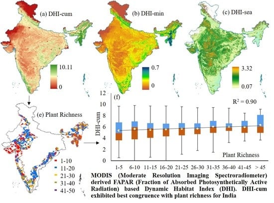
• DHI-cum representing the annual greenness was strongly correlated with the plant richness thereby emerging as a suitable indicator to monitor the plant diversity.

References

1. Foley, J.A.; Levis, S.; Costa, M.H.; Cramer, W.; Pollard, D. Incorporating dynamic vegetation cover within global climate models. Ecol. Appl. 2000, 10, 1620–1632. [Google Scholar] [CrossRef]
2. Cui, L.; Shi, J. Temporal and spatial response of vegetation NDVI to temperature and precipitation in eastern China. J. Geogr. Sci. 2010. [Google Scholar] [CrossRef]
3. Wang, R.; Gamon, J.A. Remote sensing of terrestrial plant biodiversity. Remote Sens. Environ. 2019, 231, 111218. [Google Scholar] [CrossRef]
4. Zhang, C.; Cai, D.; Guo, S.; Guan, Y.; Fraedrich, K.; Nie, Y.; Liu, X.; Bian, X. Spatial-temporal dynamics of China’s terrestrial biodiversity: A dynamic habitat index diagnostic. Remote Sens. 2016, 8, 227. [Google Scholar] [CrossRef] [Green Version]
5. Erdelen, W.R. Shaping the Fate of Life on Earth: The Post-2020 Global Biodiversity Framework. Glob. Policy 2020. [Google Scholar] [CrossRef]
6. Šímová, I.; Li, Y.M.; Storch, D. Relationship between species richness and productivity in plants: The role of sampling effect, heterogeneity and species pool. J. Ecol. 2013. [Google Scholar] [CrossRef]
7. Jetz, W.; Cavender-Bares, J.; Pavlick, R.; Schimel, D.; Davis, F.W.; Asner, G.P.; Guralnick, R.; Kattge, J.; Latimer, A.M.; Moorcroft, P.; et al. Monitoring plant functional diversity from space. Nat. Plants 2016, 2, 16024. [Google Scholar] [CrossRef] [Green Version]
8. Tucker, C.J.; Sellers, P.J. Satellite remote sensing of primary production. Int. J. Remote Sens. 1986, 7, 1395–1416. [Google Scholar] [CrossRef]
9. Waring, R.H.; Running, S.W. Forest ecosystems: Analysis at multiple scales. Choice Rev. Online 1998. [Google Scholar] [CrossRef]
10. Fensholt, R.; Sandholt, I.; Rasmussen, M.S.; Stisen, S.; Diouf, A. Evaluation of satellite based primary production modelling in the semi-arid Sahel. Remote Sens. Environ. 2006, 105, 173–188. [Google Scholar] [CrossRef]
11. Anderson, R.G.; Canadell, J.G.; Randerson, J.T.; Jackson, R.B.; Hungate, B.A.; Baldocchi, D.D.; Ban-Weiss, G.A.; Bonan, G.B.; Caldeira, K.; Cao, L.; et al. Biophysical considerations in forestry for climate protection. Front. Ecol. Environ. 2011, 9, 174–182. [Google Scholar] [CrossRef] [Green Version]
12. Jackson, R.B.; Randerson, J.T.; Canadell, J.G.; Anderson, R.G.; Avissar, R.; Baldocchi, D.D.; Bonan, G.B.; Caldeira, K.; Diffenbaugh, N.S.; Field, C.B.; et al. Protecting climate with forests. Environ. Res. Lett. 2008. [Google Scholar] [CrossRef]
13. Oindo, B.O.; Skidmore, A.K. Interannual variability of NDVI and species richness in Kenya. Int. J. Remote Sens. 2002. [Google Scholar] [CrossRef] [Green Version]
14. Huston, M.A. Biological diversity: The coexistence of species on changing landscapes. Biol. Divers. Coexistence Species Chang. Landsc. 1994. [Google Scholar] [CrossRef]
15. Muchoney, D.M. Earth observations for terrestrial biodiversity and ecosystems. Remote Sens. Environ. 2008. [Google Scholar] [CrossRef]
16. Thakur, T.K.; Padwar, G.K.; Patel, D.K.; Bijalwan, A. Monitoring land use, species composition and diversity of moist tropical environ in Achanakmaar Amarkantak Biosphere reserve, India using satellite data. Biodivers. Int. J. 2019. [Google Scholar] [CrossRef]
17. Mahanand, S.; Behera, M.D. Relationship between Field-Based Plant Species Richness and Satellite-Derived Biophysical Proxies in the Western Ghats, India. Proc. Natl. Acad. Sci. India Sect. A Phys. Sci. 2017, 87. [Google Scholar] [CrossRef]
18. Chitale, V.S.; Behera, M.D.; Roy, P.S. Deciphering plant richness using satellite remote sensing: A study from three biodiversity hotspots. Biodivers. Conserv. 2019. [Google Scholar] [CrossRef]
19. Zhou, L.; Tucker, C.J.; Kaufmann, R.K.; Slayback, D.; Shabanov, N.V.; Myneni, R.B. Variations in northern vegetation activity inferred from satellite data of vegetation index during 1981 to 1999. J. Geophys. Res. Atmos. 2001, 106, 20069–20083. [Google Scholar] [CrossRef]
20. Nemani, R.R.; Keeling, C.D.; Hashimoto, H.; Jolly, W.M.; Piper, S.C.; Tucker, C.J.; Myneni, R.B.; Running, S.W. Climate-driven increases in global terrestrial net primary production from 1982 to 1999. Science 2003. [Google Scholar] [CrossRef] [Green Version]
21. Fensholt, R.; Langanke, T.; Rasmussen, K.; Reenberg, A.; Prince, S.D.; Tucker, C.; Scholes, R.J.; Le, Q.B.; Bondeau, A.; Eastman, R.; et al. Greenness in semi-arid areas across the globe 1981-2007 - an Earth Observing Satellite based analysis of trends and drivers. Remote Sens. Environ. 2012, 121, 144–158. [Google Scholar] [CrossRef]
22. Chen, C.; Park, T.; Wang, X.; Piao, S.; Xu, B.; Chaturvedi, R.K.; Fuchs, R.; Brovkin, V.; Ciais, P.; Fensholt, R.; et al. China and India lead in greening of the world through land-use management. Nat. Sustain. 2019, 2, 122–129. [Google Scholar] [CrossRef]
23. Mondal, P.; Jain, M.; Robertson, A.W.; Galford, G.L.; Small, C.; DeFries, R.S. Winter crop sensitivity to inter-annual climate variability in central India. Clim. Chang. 2014. [Google Scholar] [CrossRef] [Green Version]
24. Mishra, N.B.; Mainali, K.P. Greening and browning of the Himalaya: Spatial patterns and the role of climatic change and human drivers. Sci. Total Environ. 2017, 587–588, 326–339. [Google Scholar] [CrossRef] [PubMed]
25. Mishra, N.B.; Chaudhuri, G. Spatio-temporal analysis of trends in seasonal vegetation productivity across Uttarakhand, Indian Himalayas, 2000-2014. Appl. Geogr. 2015, 56, 29–41. [Google Scholar] [CrossRef]
26. de Jong, R.; Verbesselt, J.; Schaepman, M.E.; de Bruin, S. Trend changes in global greening and browning: Contribution of short-term trends to longer-term change. Glob. Chang. Biol. 2012, 18, 642–655. [Google Scholar] [CrossRef]
27. Murthy, K.; Bagchi, S. Spatial patterns of long-term vegetation greening and browning are consistent across multiple scales: Implications for monitoring land degradation. Land Degrad. Dev. 2018, 29, 2485–2495. [Google Scholar] [CrossRef]
28. Chakraborty, A.; Seshasai, M.V.R.; Reddy, C.S.; Dadhwal, V.K. Persistent negative changes in seasonal greenness over different forest types of India using MODIS time series NDVI data (2001–2014). Ecol. Indic. 2018, 85, 887–903. [Google Scholar] [CrossRef]
29. Rocchini, D. Effects of spatial and spectral resolution in estimating ecosystem α-diversity by satellite imagery. Remote Sens. Environ. 2007, 111, 423–434. [Google Scholar] [CrossRef]
30. Mackey, B.; Bryan, J.; Randall, L. Australia’ s Dynamic Habitat Template for 2003; ANU Research Publications: Canberra, Australia, 2003. [Google Scholar]
31. Coops, N.C.; Wulder, M.A.; Iwanicka, D. Demonstration of a satellite-based index to monitor habitat at continental-scales. Ecol. Indic. 2009, 9, 948–958. [Google Scholar] [CrossRef]
32. Wright, D.H. Species-Energy Theory: An Extension of Species-Area Theory. Oikos 1983. [Google Scholar] [CrossRef] [Green Version]
33. Currie, D.J.; Mittelbach, G.G.; Cornell, H.V.; Field, R.; Guégan, J.F.; Hawkins, B.A.; Kaufman, D.M.; Kerr, J.T.; Oberdorff, T.; O’Brien, E.; et al. Predictions and tests of climate-based hypotheses of broad-scale variation in taxonomic richness. Ecol. Lett. 2004, 7, 1121–1134. [Google Scholar] [CrossRef]
34. Hurlbert, A.H. Linking species-area and species-energy relationships in Drosophila microcosms. Ecol. Lett. 2006. [Google Scholar] [CrossRef] [PubMed]
35. Connell, J.H.; Orias, E. The Ecological Regulation of Species Diversity. Am. Nat. 1964. [Google Scholar] [CrossRef]
36. Hu, G.; Jin, Y.; Liu, J.; Yu, M. Functional diversity versus species diversity: Relationships with habitat heterogeneity at multiple scales in a subtropical evergreen broad-leaved forest. Ecol. Res. 2014. [Google Scholar] [CrossRef]
37. Mason, N.W.H.; Mouillot, D.; Lee, W.G.; Wilson, J.B. Functional richness, functional evenness and functional divergence: The primary components of functional diversity. Oikos 2005. [Google Scholar] [CrossRef]
38. Williams, S.E.; Middleton, J. Climatic seasonality, resource bottlenecks, and abundance of rainforest birds: Implications for global climate change. Divers. Distrib. 2008. [Google Scholar] [CrossRef]
39. Coops, N.C.; Fontana, F.M.A.; Harvey, G.K.A.; Nelson, T.A.; Wulder, M.A. Monitoring of a national-scale indirect indicator of biodiversity using a long time-series of remotely sensed imagery. Can. J. Remote Sens. 2014. [Google Scholar] [CrossRef]
40. Nelson, T.A.; Coops, N.C.; Wulder, M.A.; Perez, L.; Fitterer, J.; Powers, R.; Fontana, F. Predicting climate change impacts to the canadian boreal forest. Diversity 2014, 6, 133–157. [Google Scholar] [CrossRef] [Green Version]
41. Berry, S.; Mackey, B.; Brown, T. Potential applications of remotely sensed vegetation greenness to habitat analysis and the conservation of dispersive fauna. In Proceedings of the Pacific Conservation Biology. 2007. Available online: https://www.publish.csiro.au/PC/PC070120 (accessed on 4 January 2021).
42. Berry, S.L.; Roderick, M.L. Estimating mixtures of leaf functional types using continental-scale satellite and climatic data. Glob. Ecol. Biogeogr. 2002. [Google Scholar] [CrossRef]
43. Cramer, M.J.; Willig, M.R. Habitat heterogeneity, species diversity and null models. Oikos 2005. [Google Scholar] [CrossRef]
44. Turner, M.G.; Donato, D.C.; Romme, W.H. Consequences of spatial heterogeneity for ecosystem services in changing forest landscapes: Priorities for future research. Landsc. Ecol. 2013. [Google Scholar] [CrossRef]
45. Barik, S.K.; Behera, M.D. Studies on ecosystem function and dynamics in Indian sub-continent and emerging applications of satellite remote sensing technique. Trop. Ecol. 2020, 61, 1–4. [Google Scholar] [CrossRef]
46. Zhao, M.; Heinsch, F.A.; Nemani, R.R.; Running, S.W. Improvements of the MODIS terrestrial gross and net primary production global data set. Remote Sens. Environ. 2005. [Google Scholar] [CrossRef]
47. Heinsch, F.A.; Zhao, M.; Running, S.W.; Kimball, J.S.; Nemani, R.R.; Davis, K.J.; Bolstad, P.V.; Cook, B.D.; Desai, A.R.; Ricciuto, D.M.; et al. Evaluation of remote sensing based terrestrial productivity from MODIS using regional tower eddy flux network observations. IEEE Trans. Geosci. Remote Sens. 2006. [Google Scholar] [CrossRef] [Green Version]
48. Tian, Y.; Zhang, Y.; Knyazikhin, Y.; Myneni, R.B.; Glassy, J.M.; Dedieu, G.; Running, S.W. Prototyping of MODIS LAI and FPAR algorithm with LASUR and LANDSAT data. IEEE Trans. Geosci. Remote Sens. 2000. [Google Scholar] [CrossRef] [Green Version]
49. Coops, N.C.; Wulder, M.A.; Duro, D.C.; Han, T.; Berry, S. The development of a Canadian dynamic habitat index using multi-temporal satellite estimates of canopy light absorbance. Ecol. Indic. 2008. [Google Scholar] [CrossRef]
50. Roy, P.S.; Kushwaha, S.P.S.; Murthy, M.S.R.; Roy, A.; Kushwaha, D.; Reddy, C.S.; Behera, M.D.; Mathur, V.B.; Padalia, H.; Saran, S.; et al. Biodiversity Characterisation at Landscape Level: National Assessment; Indian Institute of Remote Sensing: Dehradun, India, 2012; ISBN 8190141880. [Google Scholar]
51. Tripathi, P.; Dev Behera, M.; Roy, P.S. Optimized grid representation of plant species richness in India-Utility of an existing national database in integrated ecological analysis. PLoS ONE 2017, 12, e0173774. [Google Scholar] [CrossRef] [Green Version]
52. Schwartz, M.D.; Ahas, R.; Aasa, A. Onset of spring starting earlier across the Northern Hemisphere. Glob. Chang. Biol. 2006. [Google Scholar] [CrossRef]
53. Gaston, K.J.; Blackburn, T.M. Pattern and Process in Macroecology. 2007. Available online: https://www.wiley.com/en-ag/Pattern+and+Process+in+Macroecology-p-9780470999592 (accessed on 4 January 2021).
54. Kleijn, D.; Rundlöf, M.; Scheper, J.; Smith, H.G.; Tscharntke, T. Does conservation on farmland contribute to halting the biodiversity decline? Trends Ecol. Evol. 2011, 26, 474–481. [Google Scholar] [CrossRef]
55. Negi, V.S.; Joshi, B.C.; Pathak, R.; Rawal, R.S.; Sekar, K.C. Assessment of fuelwood diversity and consumption patterns in cold desert part of Indian Himalaya: Implication for conservation and quality of life. J. Clean. Prod. 2018, 196, 23–31. [Google Scholar] [CrossRef]
56. Vicente-Serrano, S.M.; Cabello, D.; Tomás-Burguera, M.; Martín-Hernández, N.; Beguería, S.; Azorin-Molina, C.; Kenawy, A. El Drought variability and land degradation in semiarid regions: Assessment using remote sensing data and drought indices (1982-2011). Remote Sens. 2015, 7, 4391–4423. [Google Scholar] [CrossRef] [Green Version]
57. MEA. Ecosystems and Human Well-Being. Synthesis. 2005. Available online: http://www.bioquest.org/wp-content/blogs.dir/files/2009/06/ecosystems-and-health.pdf (accessed on 4 January 2021).
58. Saikia, A. NDVI variability in North East India. Scottish Geogr. J. 2009. [Google Scholar] [CrossRef]
59. Roy, P.S.; Roy, A.; Joshi, P.K.; Kale, M.P.; Srivastava, V.K.; Srivastava, S.K.; Dwevidi, R.S.; Joshi, C.; Behera, M.D.; Meiyappan, P.; et al. Development of decadal (1985-1995-2005) land use and land cover database for India. Remote Sens. 2015, 7, 2401–2430. [Google Scholar] [CrossRef] [Green Version]
60. Pasha, S.V.; Behera, M.D.; Mahawar, S.K.; Barik, S.K.; Joshi, S.R. Assessment of shifting cultivation fallows in Northeastern India using Landsat imageries. Trop. Ecol. 2020. [Google Scholar] [CrossRef]
61. Roy, P.S.; Behera, M.D. Assessment of biological richness in different altitudinal zones in the Eastern Himalayas, Arunachal Pradesh, India. Curr. Sci. 2005, 88, 250–257. [Google Scholar]
Figure 1. (a) Biogeographic regions of India where, 1-trans-Himalaya, 2-Himalaya, 3-semi-arid, 4-arid, 5-Gangetic plain, 6-Northeast, 7-Deccan peninsula, 8-Western Ghats, 9-Coasts, 10-Islands; and Protected Areas; (b) Spatial distribution of plant richness from 0.04 ha nested quadrats that ranged from 1 to 50 in four selected biogeographic regions of India (semi-arid, eastern Ghats, Western Ghats, and Northeast) for this study.
Remotesensing 13 00159 g001
Figure 2. Cumulative dynamic habitat index (DHI-cum) derived from the monthly sum of FAPAR for a particular year is utilized to map the variation in annual greenness from 2001 to 2015 in India.
Remotesensing 13 00159 g002
Figure 3. Minimum dynamic habitat index (DHI-min) represents the minimum monthly FAPAR value in a particular year and is utilized to map the variation of minimum greenness cover from 2001 to 2015 in India.
Remotesensing 13 00159 g003
Figure 4. Seasonal dynamic habitat index (DHI-sea) is the ratio between mean and standard deviation of monthly FAPAR for a particular year was utilized to map the seasonal greenness variability from 2001 to 2015.
Remotesensing 13 00159 g004
Figure 5. The composite image of three DHI components were mapped from 2001 to 2015, where, DHI-cum was assigned with the green band, DHI-min was assigned with the blue band, and DHI-sea was assigned with the red band.
Remotesensing 13 00159 g005
Figure 6. The inter-year (2001–2015) correlation coefficient and regression coefficient calculated for each DHI components are shown as: (i) DHI-cum (a,b); (ii) DHI-min (a,b); (iii) DHI-sea (a,b), respectively.
Remotesensing 13 00159 g006
Figure 7. Representing the standard deviation map of the three DHI components from 2001 to 2015 in India, where: (a) DHI-cum SD; (b) DHI-min SD and (c) DHI-sea SD.
Remotesensing 13 00159 g007
Figure 8. Schematic representation of three DHI components using the 3-D scatter plots (DHI-cum in x-axis, DHI-min in y-axis, DHI-sea in z-axis) during 2001–2015 for the four biogeographic regions of India, where: (a) semi-arid; (b) eastern Ghats; (c) Western Ghats; (d) Northeastern region.
Remotesensing 13 00159 g008
Figure 9. The three DHI components (i) DHI-cum; (ii) DHI-min, and (iii) DHI-sea were used: (a) to map the greenness variation for India, and (b) the box plots against the field-measured plant richness data from the four Biogeographic regions of India.
Remotesensing 13 00159 g009