
SSSGAN: Satellite Style and Structure Generative Adversarial Networks


1
Satellogic, Carrer de Bailèn, 3, 1st Floor, 08010 Barcelona, Spain
2
Department of Mathematics and Informatics, Universitat de Barcelona, Gran via de les Corts Catalanes 585, 08007 Barcelona, Spain
3
Computer Vision Center, Building O, Campus UAB, Bellaterra (Cerdanyola), 08193 Barcelona, Spain
*
Author to whom correspondence should be addressed.
Remote Sens. 2021, 13(19), 3984; https://doi.org/10.3390/rs13193984
Submission received: 4 August 2021
/
Revised: 24 September 2021
/
Accepted: 29 September 2021
/
Published: 5 October 2021
(This article belongs to the Special Issue Deep Learning and Computer Vision in Remote Sensing)
Abstract
:This work presents Satellite Style and Structure Generative Adversarial Network (SSGAN), a generative model of high resolution satellite imagery to support image segmentation. Based on spatially adaptive denormalization modules (SPADE) that modulate the activations with respect to segmentation map structure, in addition to global descriptor vectors that capture the semantic information in a vector with respect to Open Street Maps (OSM) classes, this model is able to produce consistent aerial imagery. By decoupling the generation of aerial images into a structure map and a carefully defined style vector, we were able to improve the realism and geodiversity of the synthesis with respect to the state-of-the-art baseline. Therefore, the proposed model allows us to control the generation not only with respect to the desired structure, but also with respect to a geographic area.
1. Introduction
The commercialization and the advancement of the geospatial industry has led to an explosive amount of remote sensing data being collected to characterize our changing planet Earth. Public and private industries are taking advantage of this increasing availability of information in order to perform analytics and obtain more precise information about geographic areas in order to support decisions and automatize technology. Due to the increasing revisiting frequency of recently launched satellites and a fine pixel resolution (up to 30 cm per pixel, commercial ones), satellite imagery has become of interest because computer vision algorithms can capture the presence of objects in an automatic and efficient manner at a large scale. Commonly studied computer vision tasks, such as semantic and instance segmentation, object detection or height estimation, aim to address problems such as land cover classification, precision agriculture, flood detection, building, road or car detection, and at the same time help to provide information about geographic zones that can improve agriculture, navigation, retail, smart city technologies, 3D precise world reconstruction or even assistance after natural disasters.
State-of-the-art methods comprise mostly of deep learning algorithms. With the presentation of AlexNet [1] in 2012 as the winner of the ImageNet LSVRC-2012 competition by a large margin, deep networks have dominated the scene of computer vision. Due to their large number of parameters, they present a high complexity that means they require a high volume of data to correctly extract latent features from imagery, key to achieving outstanding results.
Particularly, in the field of geo-informatics and remote sensing, datasets are usually sparse, expensive and difficult to collect when it comes to tasks that require high to very high resolution images (from 1 to 0.05 m). To overcome this situation of the scarcity of images, a commonly used technique is transfer learning. This approach to training consists of using pre-trained weights as a starting point in order to improve performance and decrease training time. Pre-training is done with a highly varied high-volume dataset, so the network can extract low-level features of the world. Then, this pre-trained model is trained again with a smaller task-specific available dataset that is known as fine-tuning. This tuning can be performed by a variety of strategies that range from the most basic ones, such as freezing most of the low level layers (layers that have learnt primitive low level features) and only tuning the shallow layers, to more complex schemes that apply different learning rates to different layers.
The idea is the model to take advantage of low-level extracted features to learn more easily task-specific features in the fine-tuning. Generally, public pre-trained models are trained in datasets such as ImageNet [2] or similar ones that consist of labeled images used in visual recognition tasks (ground level visualization). Those pre-trained models are applied in totally different domains, obtaining an increment in performance with respect to training the network from scratch. For example ImageNet presents completely different visual features with respect to satellite images. Aerial-imagery contains the presence of high-frequency details and a background clutter that heavily depends on the environment, geographic zone, weather conditions, illumination, sensors and pixel resolutions. Those factors constitute a challenge itself for computer vision models to work well in a variety of cities, countries, regions, continents or even pixel resolutions.
The performance of algorithms varies markedly across geographies, image qualities and resolutions. The performance of a model applied in new areas depends, on one hand, on the target texture and topology related to cultural regions and countries [3]. Other crucial characteristics present in the image are the geographic location, weather and type of terrain. An image taken from a rural area totally differs from an urban area or from the coast. Even a specific rural area contains a different biome from a rural area of a different country/region. These points explain why it is really difficult to train a general deep network that works well with images of different locations. Additionally to the image content characteristics, there are image technical characteristics related to the methodology of extraction, such as the type of sensor, radiometry, off-nadir angle, or the atmospheric conditions at the top layers of the atmosphere.
Supervised learning techniques that use deep networks are usually trained with a large number of classes that can go from tens to thousands of labels. Thus, labeling satellite imagery is a fundamental step in the training of deep networks. Depending on the quality of labels and the resolution of the images, the cost of annotating scenes varies. Generally, the most quality satellite imagery labeling is performed by trained professionals with knowledge of GIS and geographic imagery, making this demanding annotation process slow and costly. Even the cost is tightly related to the resolution of the images; as the spatial resolution of the image increases, the cost of annotation grows accordingly. This produces a scarcity of public datasets and a bias towards most developed urban regions that have enough resources to afford this data acquisition. Scientists should make a careful selection and analysis of the datasets before starting the data annotation phase and they should also pay special attention to the quality of the labels.
When a study or research presents a model claiming to efficiently extract and detect a specific target, it usually implies that they are presenting a model trained with a dataset with specific geographic, cultural and quality conditions that perform well. In order to overcome such necessity, one possibility can be to generate a large collection of diverse synthetic images with their corresponding labels. In this case, it would be necessary to contemplate the different characteristics mentioned before, so the resulting satellite images can augment efficiently in those desired directions.
In this work, we present Satellite Style and Structured Generative Adversarial Network (SSSGAN) to generate realistic synthetic imagery (see Figure 1) based on publicly available ground truth (to get access to the models and code, please contact the authors). Particularly, we propose the use of a conditional generative adversarial network (GAN) model capable of generating synthetic satellite images constrained by two components: (1) a semantic style description of the scene; and (2) a segmentation map that defines the structure of the desired output in terms of object classes. By this way the structure and the style constraint are decoupled so the user can easily generate novel synthetic images by defining a segmentation mask of the desired foot print labels and then selecting the proportion of semantic classes expressed as number of a vector in addition to the selection of the region or city. With this generation rule the model can capture and express variability present in the satellite imagery while at the same time provides an easy-to-use generation mechanism with high expressiveness. In this work, our key contributions are as follows:
- Development of a GAN model capable of producing highly diverse satellite imagery;
- Presentation of a semantic global vector descriptor dataset based on Open Street Maps (OSM). We analyse and categorize a set of 11 classes that semantically describes the visual features that are present in satellite imagery, leveraging the public description of this crowdsourced database;
- Evaluation and study that describe the different effects of the proposed mechanisms.
1.1. Related Work
Synthetic image generation is an active research topic in the field of computer vision. A vast variety of models have been developed in the past years since the presentation in 2014 of generative adversarial networks (GAN) [4]. Even though, before and after GANS, there were numerous classical and deep learning methods, the increasing support and improvement of GAN models made this state-of-the-art technique achieve outstanding results where the synthetic generated images are hardly distinguishable from the real ones.
As mentioned before, Generative Adversarial Networks (GANS) have stated the baseline for deep generative learning. The model consists of two parts: a generator and a discriminator. The generator learns to generate synthetic, realistic images while it is trying to fool the discriminator that is responsible for distinguishing between real or fake generated images. This learning process consists of finding equilibrium in a two-player minimax game where each iteration of the generator G gets better at capturing the real data distribution thanks to the feedback of the discriminator D, which at the same time is also learning important features that help to distinguish whether the input image came from the training distribution or not. Mathematically, the generator G learns to map a latent random vector z to a generated sample tensor and tries to maximize the probability D of making a mistake, that is to say, minimizes . On the other hand, the opposite happens to D; it tries to maximize the probability of assigning the correct label and , where x is a real image and z is the latent vector
From a slightly different point of view, this process can be seen as minimizing the distance between distributions. In other words, the generator tries to approximate to the real latent distribution of images by mapping from a completely random distribution. During the training process, the Jhensen–Shannon distance is applied, measuring how far the approximated distribution is from the real one. As it is optimizing the models using gradient descent, this gradient information is back-propagated to the generator. Despite the fact that they mathematically demonstrate that there is a unique solution where D outputs for every output and G recovers the latent training data distribution, these models are unstable during training, making it laborious to train. The problem arises due to the unfair competition between generator and discriminator generating mode collapse problems, discriminators shielding infinity predictions and generators producing blank images or always producing the same sample [5]. Moreover, the basic algorithm is capable of generating up to 64 × 64 images but runs into instabilities if the size is increased. Resolution of the generated image is an important topic to address since most of the geographic and visual properties are better expressed in high-resolution so it can be used in remote-sensing applications.
Having presented the cornerstone and basics of GANs, multiple models and different variations and flavours came up, providing novel techniques, loss functions, layers or applications. Particularly, some studies such as DCGAN [6], which immediately came after the original GANs paper, added a convolutional neural network layer (CNN) in order to increase the stability of synthetic image generation. Despite it proving to generate larger images of 128 × 128 pixels, studies such as [7] report that it is not sufficient due to insufficient detail in satellite images. They also include a similar analysis to that of [4] about the input latent space, demonstrating that generators are capable of disentangling latent space dimensions by mapping particular dimensions to particular features of the generated images. Advanced techniques, such as in [5], provide new methods for training such as feature matching included in the loss, changing the objective of the loss function from maximizing the discriminator output to reducing the distance between intermediate feature maps of the discriminator extracted from real images and generator images. By doing this, the generator is forced to generate samples that produce the same feature maps in the discriminator as the real images, similar to perceptual losses [8]. They also further analyse the problem of mode collapse by proposing many strategies, such as the mini batch discriminator, where the discriminator has information from other images included in the batch, and they also propose historical averaging that adds weight to the costs and they even suggest a semi-supervised technique that trains the discriminator with labeled and unlabeled data.
Progressive Growing GAN (PGGAN) [9] proposes a method that gradually trains the generator and the discriminator until they are capable of producing large resolution images of 512 × 512 and 1024 × 1024. Their method starts by training the generator on images of 4 × 4 pixels, and by gradually adding new layers to double the generated resolution until it is capable of generating high-res images. In addition, they propose a couple of techniques that further stabilize the training and provide variation such as a minibatch standard deviation layer at the end of the discriminator, helping it to compute statistics of the batch, they propose a weight initialization and a scaling factor during runtime, and, inspired by [10], they implement a Wasserstein gradient penalty as a loss function. They propose a novel metric called Sliced Wasserstein Distance (SWD) that allows the performance of a multi scale statistical similarity between distributions of local real and fake image patches drawn from a Laplacian pyramid, providing granular quantitative results at different scales of the generated image.
In addition to the generation of large images, researchers propose novel architectures for more complex applications such as image-to-image translation, mapping from an image to an output image (conditioned generation). Pix2Pix [11] and Pix2PixHD [12] are among the first to address both problems—the image-to-image translation and high-resolution generation. Ref. [11] proposes a PatchGAN discriminator that is highly involved in posterior GAN research. The PatchGAN discriminator is applied in patches at different scales and then its outputs are averaged to produce one scalar. In combination with L1 loss that captures low-frequency information, this model, which uses fewer parameters, focuses on the high frequencies contained in each patch. Its successor, Pix2PixHD [12], is able to produce images up to 2048 × 1024 pixels with a novel multi-scale generator and discriminator, and by retaking the ideas of [5] by adding perceptual pre-trained loss. Similar to [9], they divide the training in what they refer to as a coarse-to-fine generator. This generator G is divided into two U-Net models—global generator and local enhancer . First, is trained in order to learn global characteristics at the 1024 × 512 scale. In the second phase, is added with the particularity that the encoder part is added at the beginning of and the decoder part is added at the end, leaving the in the middle. In this case, D is divided into three PatchGANs that operate at different scales. The image is downsampled in order to generate a pyramid of three scales. Then, each operates at different scales with different receptive fields, the coarse scale with a large receptive field leads to global images while the finer scale leads to finer details. The final contribution is the instance level feature embedding, a mechanism to control the generation. First, they train an encoder to find a low-dimension feature vector that corresponds to a real image. Then, they train G and D with this vector and the instance map as the conditional input. After a K-means analysis to find the cluster descriptor of each feature, the user is able to control the generation in coordination of the interpretation that the G is assigned to each dimension.
CycleGAN [13] proposes a model that learns to translate an image from one source domain to a target domain, distressing the necessity of having two paired source and target datasets. This is done by adding an inverse mapping model in the loss that reverts the first transformation applied to the input, called cycle consistency. Additionally, they reuse PatchGAN [11] as a discriminator. They conclude that, by applying the cycle loop in addition to PatchGAN, they are able to reach higher image sizes. PSGAN Progressive Structured GAN [14] is a work that adds conditionally to PGGAN. Their network is able to generate high-resolution anime characters by providing the skeleton structure of the character as an input. They take up the progressing growth by imposing the skeleton map at different scale levels while the generator and the discriminator are growing. StyleGAN [15] is GAN designed for style transfer purposes that can deal with higher resolutions and control the generation by learning high-level attributes and stochastic variations, allowing the control of the style of synthesis. They use a progressive training in conjunction with Adaptive Instance normalization layers and Wassertein gradient penalty in addition to the original GAN loss. This adapted generator learns a latent space domain and how to control features at different scales. The Perceptual Adversarial network, PAN, [16] is a general framework that is also capable of performing high-resolution image-to-image translation. Their proposal also relies on feature matching of the D, encouraging the generated images to have similar high-level features to the real ones while at the same time they use the output of D as the classical GAN loss.
Finally, we describe SPADE [17], a model that generates photorealistic imagery given a semantic map. They propose a spatially adaptive denormalization module (SPADE module), a conditional normalization layer that uses the input segmentation map to modulate the activation of the normalization layer at different scales of the generation. They demonstrate that batch normalization layers drown the signal, so they de-normalize the signal at each scale level by using SPADE layers. These layers consist simply of a convolutional layer that extracts the features of the input map and then learn by two other convolutional layers the scaling parameter at each spatial position and the scale and bias according to the input map structure. By the addition of this simple modulation and residual blocks, they obtain consistent local semantic image translations that outperform previous models such as pix2pixHD and at the same time they remove the necessity of using an encoder–decoder network. They also comment that taking a progressive growing approach makes no difference in their technique. As a discriminator, they reuse the multi-scale PatchGAN [12] with the last term replaced by Hinge loss.
In the field of remote sensing, there are not many studies focused generally on image-to-image translation using GAN. In [7], the authors described the process of applying PGAN to synthetically generate satellite images of rivers and the necessity of high-resolution image generation for remote sensing applications that can capture particular high-frequency details of this kind of image that we mentioned at the beginning of this work. Most of the work that uses GAN for remote sensing applications is conducted for cloud removal [18] or super resolution applications with GAN [19] and without GAN [20] that put special emphasis in the usage of dense skip or residual connections to propagate high-frequency signals that is particularly present in this kind of image. Works such as [21] evaluated models trained with synthetic images and demonstrated the improvement of adding them, but they do not delve into synthetic image generation techniques.
At the moment of this work, there are no vast formal studies specifically applied to the image-to-image translation of generating satellite images conditioned into the segmentation map. Despite there being works that conduct similar tasks [11,13], they rely on generally translating satellite footprints to real images as a usage example rather than conducting a complete study of these challenging tasks. It is important to remark that there are a couple of companies, such as OneView.ai (https://one-view.ai/, accessed on 3 October 2021), that base their entire business model on providing synthetic image generation services for enriching training datasets by including in their pipeline their own developed GAN model to generate synthetic images from small datasets.
1.2. Problem Formulation
Before going deeper with more complex concepts and ideas, we first provide a high-level introduction about the principal ideas around this work. Let us start by considering we have , which represents K possible classes and 0 for the background. Let be a segmentation map, a matrix where each position contains a the index of a class and H and W are the height and width of the image, respectively. Let a the -dimensional semantic global vector, where each dimension of the first V-dimensional represents a proportion of one of V semantic global classes. The remaining R-dimensional vector is a categorical (one-hot encoding) vector that represents the categorical class of the region. In this way, each scene is represented by a matrix M and a vector s. We present a deep neural network G that is capable of generating a satellite image I by receiving as an input M and s. Each pixel position of the resulting I corresponds to the label of position of m. Particularly, in this work, we simplify the problem by choosing one class segmentation map despite the fact that it could be easily adapted to more classes. We decided that M would be a building footprint map due to dataset availability and it was more than enough to validate the model and demonstrate the simplicity of generation. For the first V-dimensional part of the semantic global vector, we carefully defined 17 classes that express the number of visual cues, land use and styles relative to classes such as forest, industrial, road, and so forth (in the following sections we will explain this more in detail). We selected four cities, with remarked style, cultural and geographic properties for the second categorical R-dimensional part of the vector. We ended up with a model that—given a binary M mask with the shape and position of the buildings and a global semantic vector s that defines content related to style such as number of roads, forests, industrial land use zones and so forth, and the city/region—is capable of generating a satellite image that contains all the stylish visual cues in addition to buildings with the exact same position and shape as defined by the mask. With this control mechanism, a user can define their own segmentation mask, or can even modify the region or the amount of semantic classes for the same mask, helping it to efficiently augment a dataset with varied region/culture synthetic satellite imagery.
Finally, the model consists of a generator G of a GAN that is modified from a SPADE model [17] and a discriminator D Figure 2. Mask m and vector s are passed to generator G for generating a synthetic scene to fool the discriminator that is responsible for discerning between synthetic images and real ones.
1.3. Research Questions
The objective of this work is to propose a simple mechanism that leverages the information of public geographic databases to enhance the geographic properties of a synthetic image generated via a GAN model. While defining this mechanism, we wanted to evaluate if that enhancement would help to enrich satellite synthetic generation with finer details and properties, using a simple representation such as a 17-dimensional vector. Therefore, the main research question we address in this work is:
How can a GAN model be modified to accept rich style satellite specific properties while at the same time this information comes in a small-dimensional representation?
Additionally, this work responds to the following subsequent questions:
- How to leverage public annotation resources such as Open Street Maps to provide style information?
- How to define visual distinct land cover properties?
- Is the prior knowledge of region and style improving expressiveness of the GAN model?
2. Datasets
In this section, we describe in detail the datasets we used for training the GAN model and for the development of the semantic global vector descriptor.
2.1. Inria Aerial Image Labeling Dataset
Inria Aerial Image Labeling Dataset (Inria) [22] is a high-resolution dataset designed for pixel-wise building segmentation (Figure 3). It consists of high-resolution objectified color imagery with spatial resolution of 0.3 m/pixel that covers 810 of 5 cities (inn the training dataset):
- Vienna, Austria
- Lienz, Austria
- Chicago, USA
- Kitsap county of Washington, USA
- Austin, Texas, USA
Segmentation maps are binary images where a 1 in position means that the pixel belongs to a building and 0 that it belongs to the background class. This dataset became of interest because besides containing the structure segmentation map of buildings, its images cover a large variety of dissimilar urban and not-urban areas with different types of population, culture and urbanisation, ranging from highly urbanized Austin, Texas to the rural Tyrol region in Austria. The dataset was designed with the objective of evaluating the generalization capabilities of training in a region and extending it to images with varying illuminations, urban landscapes and times of the year. As we were interested only in the labeled images, we discarded the test set and focused on the above-mentioned cities. In consequence, our dataset consisted of 45 images of 3000 × 3000 pixels.
2.2. Open Street Map (OSM)
In 2005, OpenStreetMap (OSM) [24] was created as an open and collaborative database that provides geodata and geo-annotations. In the past few years, OSM has been widely used in several applications in geosciences, Earth observation and environmental sciences [25,26,27]. Basically, it consists of a free editable map of the world that allows its more than two million users to annotate it or to provide collected data to enrich the OSM geo-information database. Its data primarily consist of annotations at multiple semantic levels that are expressed in keys (categories) and values. Under each key they provide finer grained information in different formats depending on the object of the annotation. For example, they provide annotations of land use that describe the human usage of an area as a polygon in a geojson. Another example is the annotation of roads; they structure the road network as a graph. There are many ways to access its data such as an API or dedicated public or private geo-servers that digest and renderize the data. In our case, we decided to use a public open source server that renders and compiles all the interested information for a specific area.
Therefore, we decided to download the render for each of the images using a rasterized tile server rasterized tile server (https://github.com/gravitystorm/openstreetmap-carto/) that provides cartographic style guidelines, see Section 3.3 for more details). As we have the source code of the server, we have the mapping between pixel colour and category. We ended up listing more than 200 categories present in the render and we were capable of reducing it to only 11 classes for the global semantic vector. We will explain this procedure more in detail in the following section.
3. Methods
This section explains the methods used in this study. We will start from a more detailed analysis of the baseline model SPADE [17]. Then, we will delineate the proposed architecture modifications in order to develop SSSGAN. Next, we describe the creation of the global semantic vector. Finally, we present the metrics we used for evaluation.
3.1. SPADE
As previously explained, SPADE [17] proposed a conditional GAN architecture capable of generating high-resolution photorealistic images from a semantic segmentation map. They stated that, generally, image-to-image GANS receive the input at the beginning of the network, and consecutive convolutions and normalizations tend to wash away semantic and structural information, producing blurry and unaligned images. They propose to modulate the signal of the segmentation map at different scales of the network, producing better fidelity and alignment with the input layouts. In the following subsections, we will explain different key contributions of the proposed model.
Spatially-Adaptive Denormalization
The Spatially-Adaptive Layer is the novel contribution of this work. They demonstrated that spatial semantic information is washed away due to sequences of convolutions and batch normalization layers [28]. In order to avoid this, they propose to add these SPADE blocks that denormalize the signal in the function of the semantic map input, helping to preserve semantic spatial awareness such as semantic style and shape. Let be the segmentation mask whereas H and W are the height and width, respectively, and is a set of labels that refers to each class. Let be the activation of the i-th layer of a CNN. Let , and be the channels, height and width of the i-th layer, respectively. Assuming that the batch normalization layer is applied channel wise, and obtain and for each channel and i-th layer. The SPADE layer denormalization operation could be expressed as follows, if we consider , and be the batch size:
where and are the batch normalization parameters computed channel-wise for the batch N:
The role of the SPADE layer is to learn the scale and bias term with respect to the mask m, which they call modulation parameters in Figure 4. It is interesting to put special emphasis on the fact that modulation parameters depend on the location , thus providing spatial awareness. This spatial awareness is what differentiates this modulation with respect to batch normalization that does not consider spatial information. Those modulation parameters are expressed as a functional because the SPADE layer passes m through a series of two convolutional layers in order to learn these spatially aware parameters. The structure of layers can be seen in Figure 4.
Having defined the SPADE block, the authors reformulate the common generator architecture that uses encoder–decoder architectures [11,12]. They remove the encoder layer since the mask is not fed in the beginning of the architecture. They decided to downsample the segmentation at different scales, and fed them via SPADE blocks after each batch normalization. Then they divided the network into four upscaling segments, where the last one generates an image with the size of the mask. Each segment that defines a scale level is composed of convolutional and upscaling layers followed by SPADE residual blocks. Each SPADE residual block consists of two consecutive blocks of SPADE layers (that ingest segmentation masks that have the same dimensions as the assigned to the SPADE residual block), followed by the RELU activation layer and a 3 × 3 convolution (Figure 5). In this way, they removed the encoder and ingested information about the shape and structure of the map at each scale, obtaining a lightweight generator with fewer parameters.
As a discriminator, they decided to use a Pix2PixHD multiscale PatchGAN discriminator [12]. The task of differentiating high-resolution real images from fake ones represents a special challenge for D, since it needs to have a large receptive field that would increase network complexity. To address this problem, they used three identical PatchGAN discriminators at three different scales (factor of 2) , and . The one that operates at the coarsest scale has larger global knowledge of the image while the one that operates at the finest scale forces the generator to produce finer details, hence the loss function is the following, where k refers to the index of the three different scales:
Another particularity is that they did not use the classical GAN loss function. Instead, they used the least squared loss [29] term modification in addition to Hinge loss [30], and were demonstrated to provide more stable training and to avoid the vanishing gradient problems provided by the usage of the logistic function. Therefore, their adapted loss function is shown as follows:
Additionally, they used feature matching loss functions that we will not use in our experiments.
Finally, PatchGAN [11] is the lightweight discriminator network that is used at each scale Figure 6. It was developed with the idea that the discriminator focuses on high-frequency details while focuses on low frequencies. In consequence, they restricted the discriminator to look at particular patches to decide if it is real or fake. Consequently, the discriminator is convolved through the image by averaging its prediction of each patch into a single scalar. This allows the discriminator to have fewer parameters and focus on granular details and composition of the generated image. In fewer words, this discriminator is a simple ensemble of lightweight discriminators that reduce the input to a unique output that defines the probability of being real or fake. The authors interpreted this loss as a texture/style loss.
3.2. SSSGAN
Having studied the principal component of SPADE in detail, we were able to spot its weak points for being used in our study. The key idea of SPADE is to provide spatial semantic modulation through the SPADE layers. That property is useful for guaranteeing spatial consistency in the synthesis related to the structural segmentation map, which in our case is the building footprint, it does not apply to the global semantic vector. Our objective is to ingest global style parameters through the easy-to-generate global semantic vector, which allows the user to define the presence of semantic classes while avoiding the necessity of generating a mask with the particular location of these classes. As the semantic vector does not have spatial applicability, it cannot be concatenated, neither fed through the SPADE layer. On the other hand, we can think of this vector as a human-interpretable and already disentangled latent space. Hence, we force the network to adapt this vector as a latent space.
We replace the latent random space generator of the SPADE model for a sequence of layers that receives the global semantic vector as an input (Figure 7). In order to ingest this information, we first generate the global vector by concatenating the first V classes, the 17 visual classes and the one hot encoding vector that defines the region or area (R-dimensional). The vector goes through three consecutive multi layer perceptron (MLP) blocks of 256, 1024 and 16,384 neurons followed by an activation function. The resulting activations are reshaped to an 1024 × 4 × 4 activation volume tensor. That volume is passed to a convolutional layer and a batch normalization layer. The output is then passed to a SPADE layer that modulates this global style information with respect to the structure map. Ref. [17] suggests that the style information tends to be washed away as the network goes deeper. As a consequence, we decided to add skip connections between each of the scale blocks in channel-wise concatenation, similar to DenseNet [32]. In this way each scale block can receive the collective knowledge of previous stages, allowing the flow of the original style information. At the same time, it allows us to divide information in the way the SPADE block can focus on high-frequency spatial details, extremely important in aerial images, while the skip branch allows the flow of style and low-frequency information [20,20]. In addition, reduction blocks are added (colored in green in Figure 7) that reduce the channel dimension, which is increased by the concatenation. This helps to stack more layers for the dense connections without a significant increment of memory. Thus, it is extremely important to add those layers. Besides all of that, this structure helps to establish the training process because the dense connections also allow the gradient to be easily propagated to the lower layers, even allowing deeper network structures. This dense connection is applied by passing the volume input of each scale block with the output volume of the SPADE layer block. As the concatenation increases the channel (hence the complexity of the model), a 1 × 1 convolution layer is applied to reduce the volume.
3.3. Global Semantic Vector
In this section, we describe the creation of the global semantic vector. The key idea is to obtain a semantic description of the image that may help the generator to distinguish and pay attention to key properties present on the satellite image and it also helps to modify the image generation. In order to obtain a description, the principal idea of this work is that it can be easily generated from the OSM tags. This crowdsource tagged map is available publicly and it offers tags named by category for land use, roads, places, services. First, we download tags related to the areas of interest: Chicago, Vienna, Austin, Kitsap and Tyrol. These tags come in multiple formats, for example, land use is defined by polygons while roads are defined as a graph. We obtained more than 150 values so we decided to rasterize these tags and then to define the value that corresponds to each pixel. After that process, we analysed the results and we found different problems regarding the labels. The first problem is that urban zones were more densely and finely detailed tagged than urban zones. For example, Vienna had much more detail in tags that even individual trees were tagged (Figure 8a), while in the Tyrol region there were zones that were not even tagged. The second and more important problem was that there was no homogeneous definition of one tag in the same region or image. For example, in Chicago there were zones tagged as residential, while at the other side of the road—which has the same visual appearance—it was tagged as land (Figure 8b). Moreover, we noticed that all images of Kitsap were not annotated at all, there were roads and residential zones that were missed (Figure 8c). Finally, we come up with similar conclusions to [3], a work that only used land use information. Labels refer to human activities that are performed in specific zones. Those activities sometimes may be expressed with different visual characteristics at ground level, but from the aerial point of view those zones do not contain visual representative features. The clear example is the distinction between commercial and retail. The official definition in OSM is ambiguous, commercial refers to areas for commercial purposes, while retail is for zones where there are shops. Besides this ambiguity in definition, both areas express buildings with flat grey roofs in the aerial perspective.
Having studied all of these problems in detail, we decided to perform a manual inspection of the data and we defined a series of conventions that help to aid the previously mentioned problems. The principal idea is to create a vector in an automatic way that digests all semantic visual information so it facilitates the model to put attention on particular visual characteristics. For that reason, we decided to group all of these categories in 17 classes that have a clear visual representation despite the use. In that case, classes such as commercial and retail will constitute the same class, since while we were doing the manual visual inspection we decided that those classes are visually indistinguishable. We manually corrected zones that were not labeled and we defined a unique label for ambiguous zones, fixing the problem with residential and land labeled zones. Finally, we decided to remove images from the Kitsap region from the detest due to the scarcity in label information.
At the end of this process, we ended with the 17 classes expressed in Table 1. In order to compute the vector, we defined an index or position to each class in the vector. Having this grouping rule of classes, we processed each image by counting the amount of pixels that belong to each class (taking into account the priority of the class) and then we normalized the vector to sum 1, obtaining a distribution of classes.
More conclusions were obtained from this analysis that also coincide with the ones expressed in [3]. A specific land use, such as residential or commercial, varies in visual characteristics from region to region due to architectural and cultural factors. In order to help the network to distinguish these cultural properties, and at the same time control the generation, we added to this vector a one hot encoding selector that defines the region: Chicago, Austin, Vienna or Tyrol.
3.4. Metrics
We decided to employ two state-of-the-art perceptual metrics used in [9,17]. Since there is no ground truth, the quality of generated images is difficult to evaluate. Perceptual metrics try to provide a quantitative answer of how close the generator managed to understand and reproduce the target distribution of real images. The following metrics provide a scalar that represents the distance between distributions, and indirectly they are accessing how perceptually close the generated images are to the real ones.
3.4.1. Frechet Inception
Frechet Inception Distance (FID) [17,33] is commonly used in GAN works for measuring their image quality generation. It is a distance that measures the distance between synthetically generated images and the real distribution. Its value refers to how similar two sets of images are in terms of vector features extracted by Inception V3 model [34] trained for classification. Each image is passed through the Inception V3, and the last pooling layer prior to the output classification is extracted obtaining a feature vector of 2048 activations. These vectors are summarized as a multivariate Gaussian, computing the mean and covariance of each dimension for each image in each group. Hence, a multivariate Gaussian is obtained for each group, real and synthetic images. The resulting Frechet distance between these Gaussian distributions is the resulting score for FID. A lower score means that the two distributions are close, the generator has managed to efficiently emulate the latent real distribution.
3.4.2. Sliced Wasserstein
Sliced Wasserstein Distance (SWD) is an efficient approximation to the earth mover distance between distributions. Briefly speaking, despite being computationally inefficient, earth mover distance provides the vertical distance difference between distribution, giving an idea of the differences between densities. Ref. [9] comments that metrics such as MS-SSIM are useful for detecting coarse errors such as mode collapse, but fails to detect fine-detailed variations in color and textures. Consequently, they propose to build a Laplacian pyramid for each of the real and generated images, from 16 × 16 pixel and doubling resolution until the pyramid reaches the original dimensions. Basically, each level of the pyramid is a downsampled version of the upper level. This pyramid was constructed, having in mind that a perfect generator will synthesize similar image structures at different scales. Then, they select 16,384 images for each distribution and extract 128 patches of 7 × 7 with three RGB channels (descriptors) for each Laplacian level. This process ends up with 2.1 M of descriptors for each distribution. Each patch is normalized with respect to each color channel’s mean and standard deviation. After that, the Sliced Wasserstein Distance is applied to both sets, real and generated. Lowering the distance means that patches between both distributions are statistically similar.
Therefore, this metric provides a granular quality description at each scale. Patches at 16 × 16 similarity indicate if the sets are similar in large-scale structures, while larger scale provides more information of finer details, color or textures similarities and pixel-level properties.
4. Results
In this section, we show quantitative and qualitative results using the INRIA dataset along with our global semantic vector descriptor. We start in Section 4.1 by describing the setup of the experiment. In Section 4.2, we show the quantitative results by performing a simple ablation study. Finally, in Section 4.3, we present some qualitative results, by showing how a change in the global vector changes the style of synthesised images.
4.1. Implementation Details
The original SPADE was trained on an NVIDIA DGX1 with eight 32 GB V100 GPUs [17]. In our case, we train our network with our network with eight NVIDIA 1080Ti of 11 GB each one. This difference in terms of computational resources made us reduce the batch down to 24 images, instead of 96. Usually, training with larger batch sizes should help stabilize the training and produce better results. Regardless of this aspect, we show our approach is able to improve the generation´s expressiveness and variety with respect to the baseline, while changing the style and domain of the generated images.
We applied a learning rate of to both, the generator and the discriminator. We used ADAM optimizer with and . Additionally we applied data a few data augmentation that consisted of simply random 180° and 90° rotations. Original images were cropped to 256 × 256 patches with an overlap of 128 pixels that provide more variability. We trained each network for the same amount of 50 epochs.
4.2. Quantitative Analysis
We trained the original SPADE implementation as a baseline, which we used for referencing any quantitative improvement provided by our proposal. Then, we decided to evaluate our main architecture by using only the global semantic vector. Finally, we conducted the full approach that uses the global semantic vector and the dense connections scheme. We applied our two aforementioned metrics, Frechet (FID) Inception Metric and Sliced Wasserstein distance (SWD), for obtaining quantitative results. Table 2 shows the comparison results between different versions of the model. By a great margin, we can appreciate that the full implementation of SSSGAN, which uses the complete global semantic vector, outperforms the original baseline. The model could reduce, by more than a half, almost all the metrics. The reduction of the FID from to suggests that the generation was closer to estimating the latent distribution of the real images than the original baseline in general and global features. Moreover, it provides a more granular and detailed perspective about the generator performance at different scales. SSSGAN was able to reduce by a at the original scale, an impressive at 128 × 128 scale, a at a 64 × 64 scale, a at a 32 × 32 scale and a at 16 × 16 scale the SWD score. Our hypothesis is that, by forcing the generator to understand the already disentangled space for humans, we are providing more prior knowledge about the real distribution of the real images. During the training process, the generator can assign a correlation between the presence of particular features of the image and an increment of the global vector value. In this way the generator could produce more variable synthetic images generations and it could capture finer details structures at different scales. The generator not only reduces each metric, it could reach a constant performance in almost every scale, by learning how to generate closer to reality scale specific features.
Intermediate results that use only the semantic vector suggest that this approach provides variability to the image generation. Even though the absence of dense connections considerably reduced every score, the signal of the style that is fed into the beginning of the networks gets washed out by consistently activations modulation performed by SPADE blocks, that modulates activation only with respect to the structure of the buildings. The addition of dense connections before the modulation helps to propagate the style signal efficiently to each of the scales.
4.3. Qualitative Analysis
In this section, we show a comparison between SPADE baseline, SSSGAN with only semantic information, and the full version of SSSGAN. From Figure 9, Figure 10, Figure 11, Figure 12, Figure 13, Figure 14, Figure 15 and Figure 16, we see those networks compared in addition to the segmentation building mask, the semantic map to provide an idea of the proportion of the semantic classes and the three most influential classes of the semantic global vector. Qualitatively speaking, the full version of SPADE was able to perform a simple relation between shape of buildings and region in order to generate more consistent scenes. For example, when a structure mask is presented with the characteristic shape of Vienna’s building (Figure 16), SSSGAN can infer from the shape of building besides the information of the global vector and the region of the intended image, and generate region-specific features of the region like tree shapes, illumination, and the characteristic orange roof. Most of the time, SPADE generated flat surfaces with an absence of fine details, textures and illumination (Figure 9, Figure 10, Figure 14 or Figure 15). Another aspect to remark on relates to the style of the region is that SSSGAN was able to remarkably capture Tyrol style images (Figure 14 and Figure 15) with large light green meadows, trees, illumination and roads.
Generally speaking, SSSGAN demonstrated its vast ability to capture style and context related to each of the four regions. For example, in contrast to the baseline, SSSGAN was able to produce a detailed grass style of Tyrol and differentiate subtle tree properties of Austin and Chicago. In general, visual inspection of the generated images suggest that SSSGAN was able to capture railway track, roads and even the consistent generation of cars as in Figure 9.
Another remarkable point is the consistent shadowing of the scenes; it can be appreciated in every scene that the network is able to generate consistent shadows among every salient feature such as trees or buildings. Finally, we can see that networks have difficulties in generating long rectified lines. The reason is that the building mask contains imperfect annotated boundaries that the networks reproduce and the adversarial learning procedure does not detect and therefore do not know how to overcome.
In Figure 17, we show the generation capabilities. We increment the presence of four categories while diminishing the others in a Chicago building footprint. At the same time, we show how this generation mechanism is expressed in each region by changing the one hot encoded area vector. Efficiently, we see how each row contains a global style color palette related to the region. For example, the row of the Tyrol region in Figure 17 presents a global greenish style that is common in that region, while the trow of Chicago presents brownish and diminished colors. The increment of forest efficiently Figure 18 increases the presence of trees while the increment of industrial category tends to generate grey flat roofs over the buildings. It is important to remark that the style of the semantic category is captured, despite it does not show enough realism due to incompatibilities of building shapes with this specific style. For instance, when increasing industrial over a mask of residential houses of Chicago, the network is able to detect buildings and provide them a grey tonality, but is not providing finer details to these roofs because it is not relating the shape and dimensions of that building with respect to the increased style. Nevertheless, we can efficiently corroborate changes in style and textures by manipulating the semantic global vector.
Finally, we show in Figure 19 some negative results. In Figure 19a, we show two different cases using our semantic+dense model. On the left, the model fails at generating cars. The top example marked in red seems to be a conglomerate of pixels rather than a row of cars. On the other side, the bottom example marked in red seems like an uncompleted car. On the right image, the transition between buildings and the ground is not properly defined. Figure 19b shows a clear example where the semantic model is actually performing better than the semantic+dense version. In the latter case, the division that usually splits the roof in half (in a Vienna-scenario) tends to disappear along the roof. Moreover, one can hardly see the highway. Figure 19c shows an example where both semantic and semantic+dense, fail at properly generating straight and consistent roads. Thus, although in general, the results look promising, small objects and buildings geometry could be further improved. Hence, to mitigate some of the failures we were describing above, a geometrical constraint for small objects and buildings could be incorporated into the model, either during the training phase or as a post-processing stage.
4.4. Conclusions
Global high resolution images with corresponding ground truth are difficult to obtain due to the infrastructure and cost required to acquire and label them, respectively. In order to overcome this issue, we present a novel method, SSSGAN, which integrates a mechanism capable of generating realistic satellite images, improving the semantic features generation by leveraging publicly available crowd sourced data from OSM. These static annotations, which purely describe a scene, can be used to enhance satellite image generation by encoding it in the global semantic vector. We also demonstrate that the use of this vector, in addition to the architecture proposed in this work, permits SSSGAN to effectively increase the expressiveness capabilities of the GAN model. In the first place, we manage to outperform the SPADE model in terms of FID and SWD metrics, meaning the generator was able to better approximate the latent real distribution of real images. By evaluating the SWD metric at multiple scales, we further show the consistent increment in terms of diversity at different scale levels of the generation, from fine to coarse details. In the qualitative analysis, we perform a visual comparison between the baseline and our model, comparing the increment in diversity and region-culture styles. We finish our analysis by showing the effectiveness of manipulating the global semantic vector. This brings to light the vast potential of the proposed approach. We hope this work will encourage future synthetic satellite image generation studies that will help with a better understanding of our planet.
Author Contributions
Conceptualization, J.M. and S.E.; methodology, J.M. and S.E; validation, J.M. and S.E.; investigation, J.M. and S.E.; writing—review and editing, J.M. and S.E.; supervision, J.M. and S.E. All authors have read and agreed to the published version of the manuscript.
Funding
This work was supported by the European Regional Development Fund (ERDF) and the Spanish Government, Ministerio de Ciencia, Innovación y Universidades—Agencia Estatal de Investigación—RTC2019-007434-7; and partially supported by the Spanish project PID2019-105093GB-I00 (MINECO/FEDER, UE) and CERCA Programme/Generalitat de Catalunya), and by ICREA under the ICREA Academia programme.
Data Availability Statement
The data used in this work was publicly available.
Acknowledgments
Due to professional conflicts, one of the contributors of this work, Emilio Tylson, requested to not appear in the list of authors. He was involved in the following parts: validation, software, investigation, data curation, and writing—original draft preparation. We would also like to thank Guillermo Becker, Pau Gallés, Luciano Pega and David Vilaseca for their valuable input.
Conflicts of Interest
The authors declare no conflict of interest. The funders had no role in the design of the study; in the collection, analyses, or interpretation of data; in the writing of the manuscript, or in the decision to publish the results.
References
- Krizhevsky, A.; Sutskever, I.; Hinton, G.E. Imagenet classification with deep convolutional neural networks. Adv. Neural Inf. Process. Syst. 2012, 25, 1097–1105. [Google Scholar] [CrossRef]
- Deng, J.; Dong, W.; Socher, R.; Li, L.J.; Li, K.; Li, F.-F. Imagenet: A large-scale hierarchical image database. In Proceedings of the 2009 IEEE Conference on Computer Vision and Pattern Recognition, Miami, FL, USA, 20–25 June 2009; pp. 248–255. [Google Scholar]
- Albert, A.; Kaur, J.; Gonzalez, M.C. Using convolutional networks and satellite imagery to identify patterns in urban environments at a large scale. In Proceedings of the 23rd ACM SIGKDD International Conference on Knowledge Discovery and Data Mining, Halifax, NS, USA, 13–17 August 2017; pp. 1357–1366. [Google Scholar]
- Goodfellow, I.J.; Pouget-Abadie, J.; Mirza, M.; Xu, B.; Warde-Farley, D.; Ozair, S.; Courville, A.; Bengio, Y. Generative adversarial networks. arXiv 2014, arXiv:1406.2661. [Google Scholar]
- Salimans, T.; Goodfellow, I.; Zaremba, W.; Cheung, V.; Radford, A.; Chen, X. Improved techniques for training gans. arXiv 2016, arXiv:1606.03498. [Google Scholar]
- Radford, A.; Metz, L.; Chintala, S. Unsupervised representation learning with deep convolutional generative adversarial networks. arXiv 2015, arXiv:1511.06434. [Google Scholar]
- Gautam, A.; Sit, M.; Demir, I. Realistic River Image Synthesis using Deep Generative Adversarial Networks. arXiv 2020, arXiv:2003.00826. [Google Scholar]
- Zhang, R.; Isola, P.; Efros, A.A.; Shechtman, E.; Wang, O. The unreasonable effectiveness of deep features as a perceptual metric. In Proceedings of the IEEE Conference on Computer Vision and Pattern Recognition, Salt Lake City, UT, USA, 18–23 June 2018; pp. 586–595. [Google Scholar]
- Karras, T.; Aila, T.; Laine, S.; Lehtinen, J. Progressive growing of gans for improved quality, stability, and variation. arXiv 2017, arXiv:1710.10196. [Google Scholar]
- Arjovsky, M.; Chintala, S.; Bottou, L. Wasserstein generative adversarial networks. In Proceedings of the 34th International Conference on Machine Learning, Sydney, NSW, Australia, 6–11 August 2017; pp. 214–223. [Google Scholar]
- Isola, P.; Zhu, J.Y.; Zhou, T.; Efros, A.A. Image-to-image translation with conditional adversarial networks. In Proceedings of the IEEE Conference on Computer Vision and Pattern Recognition, Honolulu, HI, USA, 21–26 July 2017; pp. 1125–1134. [Google Scholar]
- Wang, T.C.; Liu, M.Y.; Zhu, J.Y.; Tao, A.; Kautz, J.; Catanzaro, B. High-resolution image synthesis and semantic manipulation with conditional gans. In Proceedings of the IEEE Conference on Computer Vision and Pattern Recognition, Salt Lake City, UT, USA, 18–23 June 2018; pp. 8798–8807. [Google Scholar]
- Zhu, J.Y.; Park, T.; Isola, P.; Efros, A.A. Unpaired image-to-image translation using cycle-consistent adversarial networks. In Proceedings of the IEEE International Conference on Computer Vision, Venice, Italy, 22–28 October 2017; pp. 2223–2232. [Google Scholar]
- Hamada, K.; Tachibana, K.; Li, T.; Honda, H.; Uchida, Y. Full-body high-resolution anime generation with progressive structure-conditional generative adversarial networks. In Proceedings of the European Conference on Computer Vision (ECCV) Workshops, Munich, Germany, 8–14 September 2018. [Google Scholar]
- Karras, T.; Laine, S.; Aila, T. A style-based generator architecture for generative adversarial networks. In Proceedings of the IEEE/CVF Conference on Computer Vision and Pattern Recognition, Long Beach, CA, USA, 15–20 June 2019; pp. 4401–4410. [Google Scholar]
- Wang, C.; Xu, C.; Wang, C.; Tao, D. Perceptual adversarial networks for image-to-image transformation. IEEE Trans. Image Process. 2018, 27, 4066–4079. [Google Scholar] [CrossRef] [PubMed] [Green Version]
- Park, T.; Liu, M.Y.; Wang, T.C.; Zhu, J.Y. Semantic image synthesis with spatially-adaptive normalization. In Proceedings of the IEEE/CVF Conference on Computer Vision and Pattern Recognition, Long Beach, CA, USA, 15–20 June 2019; pp. 2337–2346. [Google Scholar]
- Singh, P.; Komodakis, N. Cloud-gan: Cloud removal for sentinel-2 imagery using a cyclic consistent generative adversarial networks. In Proceedings of the IGARSS 2018—2018 IEEE International Geoscience and Remote Sensing Symposium, Valencia, Spain, 22–27 July 2018; pp. 1772–1775. [Google Scholar]
- Wang, Z.; Jiang, K.; Yi, P.; Han, Z.; He, Z. Ultra-dense GAN for satellite imagery super-resolution. Neurocomputing 2020, 398, 328–337. [Google Scholar] [CrossRef]
- Salvetti, F.; Mazzia, V.; Khaliq, A.; Chiaberge, M. Multi-image Super Resolution of Remotely Sensed Images using Residual Feature Attention Deep Neural Networks. arXiv 2020, arXiv:2007.03107. [Google Scholar]
- Shermeyer, J.; Hossler, T.; Van Etten, A.; Hogan, D.; Lewis, R.; Kim, D. Rareplanes: Synthetic data takes flight. In Proceedings of the IEEE/CVF Winter Conference on Applications of Computer Vision, Waikola, HI, USA, 5–9 January 2021; pp. 207–217. [Google Scholar]
- Maggiori, E.; Tarabalka, Y.; Charpiat, G.; Alliez, P. Can Semantic Labeling Methods Generalize to Any City? The Inria Aerial Image Labeling Benchmark. In Proceedings of the IEEE International Geoscience and Remote Sensing Symposium (IGARSS), Fort Worth, Texas, USA, 23–28 July 2017. [Google Scholar]
- Ma, J.; Wu, L.; Tang, X.; Liu, F.; Zhang, X.; Jiao, L. Building extraction of aerial images by a global and multi-scale encoder-decoder network. Remote Sens. 2020, 12, 2350. [Google Scholar] [CrossRef]
- OpenStreetMap Contributors. Available online: https://www.openstreetmap.org (accessed on 3 October 2021).
- Kang, J.; Körner, M.; Wang, Y.; Taubenböck, H.; Zhu, X.X. Building instance classification using street view images. ISPRS J. Photogramm. Remote Sens. 2018, 145, 44–59. [Google Scholar] [CrossRef]
- Baier, G.; Deschemps, A.; Schmitt, M.; Yokoya, N. Synthesizing Optical and SAR Imagery From Land Cover Maps and Auxiliary Raster Data. IEEE Trans. Geosci. Remote Sens. 2021. [Google Scholar] [CrossRef]
- Vargas-Munoz, J.E.; Srivastava, S.; Tuia, D.; Falcão, A.X. OpenStreetMap: Challenges and Opportunities in Machine Learning and Remote Sensing. IEEE Geosci. Remote Sens. Mag. 2021, 9, 184–199. [Google Scholar] [CrossRef]
- Ioffe, S.; Szegedy, C. Batch normalization: Accelerating deep network training by reducing internal covariate shift. In Proceedings of the 32nd International Conference on International Conference on Machine Learning, Lille, France, 7–9 July 2015; pp. 448–456. [Google Scholar]
- Mao, X.; Li, Q.; Xie, H.; Lau, R.Y.; Wang, Z.; Paul Smolley, S. Least squares generative adversarial networks. In Proceedings of the IEEE International Conference on Computer Vision, Venice, Italy, 22–29 October 2017; pp. 2794–2802. [Google Scholar]
- Miyato, T.; Kataoka, T.; Koyama, M.; Yoshida, Y. Spectral normalization for generative adversarial networks. arXiv 2018, arXiv:1802.05957. [Google Scholar]
- Ganokratanaa, T.; Aramvith, S.; Sebe, N. Unsupervised anomaly detection and localization based on deep spatiotemporal translation network. IEEE Access 2020, 8, 50312–50329. [Google Scholar] [CrossRef]
- Huang, G.; Liu, Z.; Van Der Maaten, L.; Weinberger, K.Q. Densely connected convolutional networks. In Proceedings of the IEEE Conference on Computer Vision and Pattern Recognition, Honolulu, HI, USA, 21–26 July 2017; pp. 4700–4708. [Google Scholar]
- Heusel, M.; Ramsauer, H.; Unterthiner, T.; Nessler, B.; Hochreiter, S. Gans trained by a two time-scale update rule converge to a local nash equilibrium. arXiv 2017, arXiv:1706.08500. [Google Scholar]
- Szegedy, C.; Vanhoucke, V.; Ioffe, S.; Shlens, J.; Wojna, Z. Rethinking the inception architecture for computer vision. In Proceedings of the IEEE Conference on Computer Vision and Pattern Recognition, Las Vegas, NV, USA, 27–30 June 2016; pp. 2818–2826. [Google Scholar]
Figure 1.
Synthetic images generated by SSSGAN.

Figure 2.
SPADE high level diagram. The generator takes the building footprint mask (m matrix) and the semantic global vector. It generates the synthetic image I and it is passed to the discriminator to determine if it is fake or real.
Figure 2.
SPADE high level diagram. The generator takes the building footprint mask (m matrix) and the semantic global vector. It generates the synthetic image I and it is passed to the discriminator to determine if it is fake or real.

Figure 3.
Inria building datasets sample [23].
Figure 3.
Inria building datasets sample [23].

Figure 4.
(a) SPADE block internal architecture. (b) SPADE Residual block (SPADE ResBlk).

Figure 5.
SPADE main architecture.

Figure 6.
PatchGAN diagram [31]. The entire discriminator is applied to patches. Then, the model is convolved over the image and their results are averaged in order to obtain a single scalar.
Figure 6.
PatchGAN diagram [31]. The entire discriminator is applied to patches. Then, the model is convolved over the image and their results are averaged in order to obtain a single scalar.

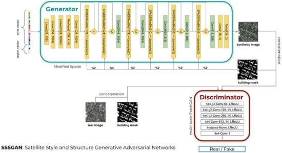
Figure 7.
SSSGAN architecture. Every linear layer is followed implicitly by Relu activation. The structure mask is downsampled to its half resolution each time it is fed to a SPADEResBlock ( referenced by ‘%2’ label).
Figure 7.
SSSGAN architecture. Every linear layer is followed implicitly by Relu activation. The structure mask is downsampled to its half resolution each time it is fed to a SPADEResBlock ( referenced by ‘%2’ label).

Figure 8.
(a) Detailed annotation of the urban area of Vienna (b) Residential area from Chicago, from one side of the annotated road is defined as residential and the other side is not annotated, despite both belongs to the same visual residential cues (c) Area of Kitsap without annotation.
Figure 8.
(a) Detailed annotation of the urban area of Vienna (b) Residential area from Chicago, from one side of the annotated road is defined as residential and the other side is not annotated, despite both belongs to the same visual residential cues (c) Area of Kitsap without annotation.

Figure 9.
Visual comparison of Austin area. Mask of building footprint and main semantic classes of the vector are shown as reference.
Figure 9.
Visual comparison of Austin area. Mask of building footprint and main semantic classes of the vector are shown as reference.

Figure 10.
Visual comparison of Austin area. Mask of building footprint and main semantic classes of the vector are shown as reference.
Figure 10.
Visual comparison of Austin area. Mask of building footprint and main semantic classes of the vector are shown as reference.

Figure 11.
Visual comparison of Austin area. Mask of building footprint and main semantic classes of the vector are shown as a reference.
Figure 11.
Visual comparison of Austin area. Mask of building footprint and main semantic classes of the vector are shown as a reference.

Figure 12.
Visual comparison of Chicago area. Mask of building footprint and main semantic classes of the vector are shown as reference.
Figure 12.
Visual comparison of Chicago area. Mask of building footprint and main semantic classes of the vector are shown as reference.

Figure 13.
Visual comparison of Chicago area. Mask of building footprint and main semantic classes of the vector are shown as a reference.
Figure 13.
Visual comparison of Chicago area. Mask of building footprint and main semantic classes of the vector are shown as a reference.

Figure 14.
Visual comparison of Tyrol area. Mask of building footprint and main semantic classes of the vector are shown as a reference.
Figure 14.
Visual comparison of Tyrol area. Mask of building footprint and main semantic classes of the vector are shown as a reference.

Figure 15.
Visual comparison of Tyrol area. Mask of building footprint and main semantic classes of the vector are shown as a reference.
Figure 15.
Visual comparison of Tyrol area. Mask of building footprint and main semantic classes of the vector are shown as a reference.

Figure 16.
Visual comparison of Vienna area. Mask of building footprint and main semantic classes of the vector are shown as a reference.
Figure 16.
Visual comparison of Vienna area. Mask of building footprint and main semantic classes of the vector are shown as a reference.

Figure 17.
Original building footprint is from Chicago. Each row shows the generation for that Chicago footprint mask in different regions. First column uses the original global semantic vector. Second column the grass category is increased. Third column forest class is increased. Finally, the fourth column industrial class is increased.

Figure 18.
Finer observation of the increment of grass class and forest class.

Figure 19.
Negative results. (a) Two different generated images using our semantic+dense model. (b) Two generated images using the same footprint input, semantic model output on the left, semantic+dense output on the right. (c) Two generated images using the same footprint input, semantic model output on the left, semantic+dense model output on the right.


Table 1.
CNN Performance Long Format.
| Semantic Category | OSM Tag | Index |
|---|---|---|
| grass | grass, heath, golf_course, farmland, … | 1 |
| forest | forest, forest-text, orchard, scrub, … | 2 |
| residential | residential, residential-line, land-color, … | 3 |
| commercial | commercial, commercial-line, retail, … | 4 |
| industrial | industrial, industrial-line, wastewater_plant, … | 5 |
| parking | garages, parking, … | 6 |
| construction | construction, construction_2, built-up-z12, quarry, … | 7 |
| sports | pitch | 8 |
| highway | motorway, primary, secondary, … | 9 |
| rail | motorway, primary, secondary, … | 10 |
| road | living_street, residential, … | 11 |
| footway | footway, pedestrian, … | 12 |
| religious | cemetery, religius, … | 13 |
| motorway | motorway, trunk, … | 14 |
| water | water, … | 15 |
| allotments | allotments, … | 16 |
| block | block, … | 17 |
Table 2.
Performance different SSSGAN versions with respect to SPADE baseline.
| Model | FID | SWD-256 | SWD-128 | SWD-64 | SWD-32 | SWD-16 |
|---|---|---|---|---|---|---|
| baseline | 53.19 | 338.53 | 474.08 | 486.17 | 474.08 | 665.29 |
| semantic(ours) | 38.17 | 207.64 | 206.29 | 241.29 | 232.02 | 404.96 |
| semantic+dense(ours) | 22.36 | 148.93 | 111.89 | 153.75 | 173.86 | 355.16 |
Model comparison. Baseline refers to the original SPADE implementation [17]. While “semantic” refers to the SSSGAN with only style vector and “semantic+dense” is the full model SSSGAN with global semantic vector and dense connection structure.
Publisher’s Note: MDPI stays neutral with regard to jurisdictional claims in published maps and institutional affiliations. |
© 2021 by the authors. Licensee MDPI, Basel, Switzerland. This article is an open access article distributed under the terms and conditions of the Creative Commons Attribution (CC BY) license (https://creativecommons.org/licenses/by/4.0/).
Share and Cite
MDPI and ACS Style
Marín, J.; Escalera, S. SSSGAN: Satellite Style and Structure Generative Adversarial Networks. Remote Sens. 2021, 13, 3984. https://doi.org/10.3390/rs13193984
AMA Style
Marín J, Escalera S. SSSGAN: Satellite Style and Structure Generative Adversarial Networks. Remote Sensing. 2021; 13(19):3984. https://doi.org/10.3390/rs13193984
Chicago/Turabian StyleMarín, Javier, and Sergio Escalera. 2021. "SSSGAN: Satellite Style and Structure Generative Adversarial Networks" Remote Sensing 13, no. 19: 3984. https://doi.org/10.3390/rs13193984
Note that from the first issue of 2016, this journal uses article numbers instead of page numbers. See further details here.