Monitoring Cropping Intensity Dynamics across the North China Plain from 1982 to 2018 Using GLASS LAI Products


1
Key Laboratory of Digital Earth Science, Aerospace Information Research Institute (AIR), Chinese Academy of Sciences (CAS), Beijing 100094, China
2
University of Chinese Academy of Sciences, Beijing 100049, China
3
Agricultural Information Institute, Chinese Academy of Agricultural Sciences, Beijing 100081, China
4
International Centre on Space Technologies for Natural and Cultural Heritage (HIST) under the Auspices of UNESCO, Beijing 100094, China
*
Author to whom correspondence should be addressed.
Remote Sens. 2021, 13(19), 3911; https://doi.org/10.3390/rs13193911
Submission received: 23 August 2021
/
Revised: 21 September 2021
/
Accepted: 22 September 2021
/
Published: 30 September 2021
(This article belongs to the Section Remote Sensing in Agriculture and Vegetation)
Abstract
:China is a large grain producer and consumer. Thus, obtaining information about the cropping intensity (CI) in cultivated land, as well as understanding the intensified utilization of cultivated land, is important to ensuring an increased grain production and food security for China. This study aims to detect and map the changes in CI over a period of 36 years across China’s core grain-producing area—the North China Plain (NCP)— using remotely sensed leaf area index (LAI) time series data acquired by the Global LAnd Surface Satellite (GLASS) products. We first selected 2132 sample points that consisted entirely, or almost entirely, of cultivated cropland from all pixels; the biennial LAI curves for the sample points were then extracted; the Savitzky–Golay filter and second-order difference algorithm were then applied to reconstruct the biennial LAI curves and obtain the number of peaks in these curves. In addition, the multiple cropping index (MCI) was calculated to represent the CI. Finally, the spatial distribution of the CI of cultivated land on the NCP was mapped from 1982 to 2018 using a geo-statistical kriging approach. Spatially, the results indicate that the CI of cultivated land over the NCP exhibits a distinct spatial pattern that conforms to “high in the south, low in the north”. The single cropping system (SCS) mainly occurred in the higher latitude area ranging from 37.04°N to 42.54°N, and the double cropping system (DCS) mainly existed in the lower latitude area between 31.95°N and 39.97°N. Temporally, the CI increased over the study period, but there were some large fluctuations in CI from 1982 to 1998 and it maintained relatively stable since 2000. Across the NCP, 68.14% of cultivated land experienced a significant increase in CI during the 36-year period, while only 3.87% showed a significant decrease. We also found that, between 1982 and 2018, the northern boundary of the area for DCS underwent a significant westward expansion and northward movement. Our results show a good degree of consistency with statistical data and previous research and also help to improve the reliability of satellite-based identification of CI using low spatial resolution LAI products. The results provide important information that can be used for analyzing and evaluating the rational utilization of cultivated land resources; thus, ensuring food security and realizing agricultural sustainability not only for the NCP, but for China as a whole. These results also highlight the value of satellite remote sensing to the long-term monitoring of cropping intensity at large scales.
1. Introduction
As a result of climate change, there has been an obvious increase in temperature in recent years [1], and this has had a great impact on the utilization of regional agricultural resources (including cultivated land) and agricultural production [2,3,4]. In the era of increasingly fierce conflict between human beings and the land, understanding the temporal–spatial variations in regional cropping intensity (CI) is of great significance to the management of grain production and agricultural production [5,6], as well as to measures taken to deal with climate change. All of these are important to ensuring the safety of food production and to the promotion of modern agricultural techniques and sustainable development at the regional scale [7,8,9,10].
CI is often measured by the multiple cropping index (MCI), which is the planting frequency of crops in the same farmland in one year; MCI also equals to the ratio of the total sown area of crops to the arable land area in one year and can be obtained by three main methods [11]. These include a statistical method based on the ratio of the crop-sown area to the total cultivated area, the potential estimation model, which is based on an analysis of the factors that limit increases in the MCI, and the spatial-monitoring method, which is based on a long-term series of remote sensing data [12]. The use of remote sensing has become the main method for monitoring regional MCI because of its advantages; i.e., the low cost, wide coverage and high temporal resolution [13,14]. The extraction of MCI based on remote sensing data is, in fact, effective in some areas; however, the effectiveness of this approach is closely related to the spatial resolution of the remote sensing data and the complexity of the regional land-use patterns [15]. Therefore, for fragmented cultivated areas, it is hard to improve the accuracy of mapping CI based on moderate- or low-resolution remote sensing data [16,17].
Nowadays, time series of the Normalized Difference Vegetation Index (NDVI) and the Enhanced Vegetation Index (EVI) are the main sources used for monitoring the CI both in China and in other countries. It can be seen that the research of CI using NDVI data is nearly mature [18,19,20,21,22,23,24], and it has also achieved good results using EVI data [25,26,27,28,29,30]. However, as a biophysical variable, LAI can also characterize the phenological characteristics of green vegetation, but there is little or almost no research on the CI of cultivated land based on LAI. Compared with the saturation problem of the NDVI under high density vegetation and the lack of a high-quality EVI product prior to 2000 [31], it is more advantageous to choose the time series LAI for measuring CI in the long-term. Meanwhile, if these approaches are mainly based on low spatial resolution images, they would inevitably lead to the observations of mixed cropping practices rather than a pure cropping practice within each pixel [15]. In order to solve the issue, several studies were carried out to measure the CI by employing the finer spatial resolution images, e.g., Landsat and Sentinel observations in recent years [32,33,34,35]. Unfortunately, the temporal sampling period of Landsat series is just 16 or 18 days, while the crop growth is fast-changing; this is especially problematic during the critical growth period. It means that the annually available cloud-free images merely provided by a single Landsat sensor would hardly satisfy an effective observation of CI throughout a year for an entire region, especially for the areas with persistent clouds [15,36,37]. In addition, the Sentinel series has only been available since after 2014, which could not meet the research needs of more than seven years since then.
The North China Plain (NCP) is China’s core grain-producing area. Thus, the timely acquisition of information about the dynamic changes in CI using remote sensing is of practical significance to the assessment of CI and to food security in the NCP. Due to the high degree of urbanization and land fragmentation, remote sensing data of the NCP are seriously affected by the mixed pixel problem [38]. A method that can minimize the errors due to mixed pixels caused by land fragmentation is adopted in this study. By means of this study, we hope to provide a basis for the analysis and evaluation of the rational utilization of regional land resources; thus, ensuring food security and aiding ecological protection for the NCP and China as a whole. At the same time, we aim to lay a solid scientific reference for decision-making related to regional agricultural planning.
2. Materials and Methods
2.1. Study Area
The NCP mainly consists of the provinces of Hebei, Shandong and Henan as well as the municipalities of Beijing and Tianjin; it also includes parts of northern Jiangsu and Anhui provinces [39]. In this study, our study area was located mainly between 32°N and 42°N and 113°E and 120°E in Lambert conformal conic projection; thus, excluding the parts of the plain that are in Jiangsu and Anhui provinces (Figure 1). With flat terrain, deep and fertile soil and a great number of rivers and lakes, the NCP is a typical alluvial plain that has an altitude of less than 50 meters over most of its area [40]. The annual average temperature is 12–15 °C, with an annual accumulated temperature (≥0 °C) of 4100–5400 °C and an annual frost-free period of 190–220 days. The average annual precipitation is 500–1000 mm. These climate conditions meet the requirements of a one-year double cropping system (DCS) [41].
The study area is an important crop production region for China, and its cultivated area accounts for 18% of the total area of cultivated land in China; the area’s grain output accounts for 21% of national agricultural production [40]. Dryland farming is the main farming system used on the NCP; the main crops are wheat and maize. Excepting the single cropping system (SCS) over one year in parts of northern region in Beijing and Hebei province and the triple cropping system (TCS) over two years in part of southern Henan province, the DCS with winter wheat and summer maize planting is the main farming system in NCP. This forms a comprehensive agricultural system with well-developed irrigation and features of grain and cotton cultivation.
2.2. Data
2.2.1. Remotely Sensed LAI Data
The remotely sensed LAI data used in this study were GLASS LAI data for the period 1982 to 2018, provided by the GLCF (Global Land Cover Facility) (http://glass-product.bnu.edu.cn/, accessed 3 on May 2020) (Table 1). The GLASS LAI dataset has a temporal resolution of 8 days and is a 37-year (1981–2018) Leaf Area Index remote sensing product [42,43,44]. The LAI product covering the period 1981–1999 has a spatial resolution of 0.05° × 0.05° and uses a geographic projection; the LAI data for 2000 to 2018 uses an Integrated Sinusoidal projection with three spatial resolutions of 0.05° × 0.05°, 1 × 1 km and 500 × 500 m [45,46,47]. In this study, the GLASS LAI data with a spatial resolution of 0.05° × 0.05° were used to maintain continuity.
2.2.2. Land Use Data
The land use dataset was acquired from China’s Land Use Remote Sensing Monitoring Database for 1980, 1990, 1995, 2000, 2005, 2010, 2015 and 2018. This database has a scale of 1:100,000 and was provided by the Science Data Center of Resources and Environment, Chinese Academy of Sciences (http://www.resdc.cn, accessed on 3 May 2020). We used these data to extract location and area information related to cultivated land on the NCP. Based on these information, we extracted the data of unchanged cultivated land in the land use dataset to obtain spatio-temporal information about the CI over the NCP; in this way, it could avoid the errors for mapping CI caused by the distribution and area differences of cultivated land in different years.
2.2.3. Statistical Data
Statistical agricultural data in province scale, including the cultivated land area and total sown area in the study region, were obtained from the China Statistical Yearbook (http://www.stats.gov.cn/tjsj/ndsj/, accessed on 11 August 2020) and the Beijing, Tianjin, Hebei, Shandong and Henan Statistical Yearbooks for 1982 to 2018. These data were used to calculate the reference MCI for each subregion as well as the whole study area, and to comparatively analyze and validate the CI extracting results using our proposed method.
2.3. Algorithms for Identifying the Cropping Intensity
For crops, long-time series of the LAI can describe the characteristics of annual or interannual growth changes and reflect changes in the life cycles of crops [47,48]. From sowing, emergence, jointing and heading to harvesting, the LAI values of crops also undergo a dynamic process of increase to peak to decrease. Therefore, by constructing LAI time series for crop growth and calculating the MCI from the number of peaks in these curves, the CI of cultivated land can be monitored [47]. The algorithm based on the long-term GLASS LAI series that was used for determining the CI of cultivated land is shown below (Figure 2).
2.3.1. Using Spatial Sampling to Obtain Sample Points in Pure Pixels of Cultivated Land Pixels
Based on the information about unchanged cultivated land on the NCP that was extracted from the land use dataset in 1980, 1990, 1995, 2000, 2005, 2010, 2015 and 2018, 3500 cultivated land sample points were randomly selected using a gridded spatial sampling strategy (by on grid per 5 km × 5 km; 18,308 grids in total); these, then, formed the preliminary sample used in this study. Next, each sample point was validated and verified using high-resolution imagery (e.g., Google Earth version 7.1.2.2019 imagery) and pixels that consisted of more than 80% cultivated land were then selected, meaning that all of these pixels were either pure or nearly pure cultivated land pixels. In this way, 2132 cultivated land sample points covering the NCP were obtained (Figure 1B), of which 110 were the validation sample.
The land use on the NCP was highly fragmented and, to a certain extent, this sampling method could not only reduce the errors caused by mixed pixels in low- and medium-resolution data (i.e., GLASS LAI data) when trying to extract the CI, but also improve the accuracy of kriging spatial interpolation by increasing the density of sampling points appropriately (by one point per 250 km2 on average).
2.3.2. Extracting the Peaks of the LAI Curve
- (1)
- Smoothing of LAI time series curves
In this study, we used the Savitzky–Golay (S–G) filtering method to remove the noisy components in the long LAI time series and to reconstruct the LAI curves for crop growth in the areas of cultivated land [49]. The formula used was:
where (j = 1, …, N) is the filter LAI value, (j = 1, …, N) is the original LAI value, is the coefficient for the ith LAI value of the filter, and N is the number of convoluting integers, which is equal to the size of the smoothing window (2m + 1). The smoothing array consists of 2m + 1 points, where m is the half-width of the smoothing window [50,51]. The can be obtained from Steinier et al. [52].
- (2)
- Extracting the number of peaks in the LAI curves
We employed a second-order difference algorithm to identify the number of peaks in the reconstructed LAI curves [53,54] and, then, extracted the MCI for cultivated land within the NCP from 1982 to 2018 [55]:
where is the LAI value of a sampling pixel with i being the time series phase for the GLASS LAI imagery. , and are the detected parameters in Equations (2)–(4), respectively; the meanings of these are explained in Section 3.2.
2.3.3. CI Estimation
- (1)
- Calculating the MCIs of the sample points
Based on the relationship between the LAI time series for cultivated land and the MCIs, the MCIs could easily be converted to the number of peaks in the LAI curves [56]. Given the number of peaks for a given sample point, the number of peaks in the LAI curves of the crops (i.e., the MCIs of the cultivated land sample points) could be obtained from the ratio of the number of peaks to the total number of sample points:
where represents the frequency of wave peaks in the ith year, is the number of peaks in the LAI curves for all of the sample points during the ith year, is the total number of sample points during the ith year and j (equal to 1, 2, 3,…) is the sample point number.
- (2)
- Spatial mapping of CI
In this study, the numeric value of MCI was employed to measure the CI. Based on the MCIs of the cultivated land sample points, time series maps showing the spatial distribution of the CI of the cultivated land on the NCP were produced using the geostatistical Kriging interpolation model. According to the characteristics of the sample data, the Ordinary Kriging model was used for the spatial interpolation [57]. The relevant equation was:
where is the measured value at the ith position, is the unknown weight of the measured value at the ith position, is the predicted position and is the number of measured values.
Following this, we performed an accuracy analysis by comparing different semivariogram models (i.e., Gaussian, spherical, exponential and linear) to select the most optimal Kriging mode for spatial interpolation [58]. Additionally, the spatial patterns of CI for the cultivated land on the NCP from 1982 to 2018 were mapped using the optimal Kriging mode; i.e., the linear Kriging mode.
3. Results
3.1. Smoothed LAI Time Series Curves
The S-G filtering model was used to smooth and reconstruct the LAI time series, and the results were satisfactory. The reconstructed LAI curves for the sample points on cultivated land reflected the processes of crop growth and development well, and the number of peaks in the curves was clear; thus, allowing the multiple cropping on the NCP to be accurately characterized (Figure 3). Figure 3A–D shows, respectively, the LAI curves for bare or fallow land, SCS, DCS and triple cropping system. These curves contained 0, 1, 2 and 3 peaks, respectively; curves such as these were used as the basis for extracting the CI of cultivated land from remote sensing data.
3.2. Extraction Results of the Peaks of the LAI Curve and the Determination of Valid Correct Peaks
Taking the extraction of the peaks for a sample point from 1982, as an example, we obtained the results for each step of the calculation given by Equations (2)–(4) according to the principles of the second-order difference algorithm. Figure 4A shows the positions and numbers of peaks and troughs in the smoothed LAI time series, whereas Figure 4B–D shows the positions of the peaks and troughs in the curve determined using Equations (2)–(4), respectively. In this way, the complete process used to extract the number of peaks using the second-order difference algorithm can be understood.
It can be seen from Figure 4 that peak one and peak two were true peaks, while peak three was a false peak. In order to decide which were the true peaks, the following conditions were applied [59,60,61].
- The peak shown occurred between day 120 and day 300 of a year;
- In the case of a unimodal peak, the LAI value at the peak should not be less than two;
- In the case of multimodal peaks, the LAI value at the smaller peak should not be less than 40% of the value of the highest peak.
3.3. Accuracy Assessment of the CI
3.3.1. Comparison of the MCIs in This Study with Statistical Data
As the index to measure CI in this study, the extraction precision of MCI was closely related to the accuracy of the spatio–temporal change analysis for CI. The extraction accuracy of the MCI was determined by comparing the results with the statistical data for the MCI from 1982 to 2018 (the data for some years were missing) (Figure 5). Our results based on remote sensing LAI data were generally highly consistent with those derived from the statistical data. Although in 1982, 1996 and 2018, the accuracy of the CI for Beijing was less than 70%; for about 85% of the remote sensing extraction results the accuracy was more than 80% (and over 90% for 61% of the results). This showed that the results of this study were fairly consistent with the statistical data, further verifying that the CI results retrieved by remote sensing were reliable. The accuracies of MCIs are calculated by formulas (7) and (8) as follow:
where is the MCI in this study; is the MCI calculated based on statistical data; is the total sown area of crops; is the cultivated land area.
3.3.2. Comparison of the MCI in This Study with Other Research Results
Based on the MCI, comparisons were also made between the results of the current study and the monitoring results obtained by Fan and Wu [62] in 2000 and 2002 and Li et al. [26] in 2002, 2008 and 2014 (Figure 6).
It can be seen from Figure 6 that the results of this study were in good agreement with the earlier researches, especially with regard to the results obtained by Li et al. [26], for which there was an extremely small difference of less than 10% in 2014. The differences of MCI in Tianjin and Beijing were the largest, followed by Shandong Province, and the difference in Henan Province was the smallest. However, for different provinces or years, there were some slight differences between the results of our study and the others. In 2002, Henan had the greatest discrepancy between our results and the results obtained by Li et al. [26] at 28.77%. The difference was less than 5% for Hebei and Tianjin in 2002, Hebei in 2008, as well as Hebei, Henan, Beijing and Tianjin in 2014. This suggests that, overall, there was a high degree of consistency between the results of our study and those of earlier studies; however, due to various factors such as the monitoring methods used and the datasets on which the studies were based, some discrepancies remained. A comparison between the results of our study, the results of previous research and the statistical data showed that our results were closer to the statistical data than the results obtained in previous research.
3.3.3. Cross Validation for the Cropping System of Cultivated Land over the NCP
In this study, the rounded numeric value of MCI was employed to measure the cropping system (CS). The value of MCI below 150% and exceeding 50% meant it was SCS in that pixel, while the value 150–250% meant it was DCS and exceeded 50% mean TCS. We also used cross validation to verify the precision of the CS of cultivated land. Firstly, 110 samples were randomly selected from the 2132 cultivated land sample points. Based on the LAI time series data, 2090 group data of cropping systems for every two years from 1982 to 2018 were directly extracted from the 110 validated sample points. In addition, spatial data for the CS used on the NCP were also extracted from the sample points after interpolation and, then, the accuracy of the spatial mapping results was validated by analyzing the two data error matrices (Table 2).
The results showed that the overall accuracy of the spatial mapping in this study was 81.87%; comparing with accuracy for fallow fields and SCS, the precision of the user for the DCS was generally high, while the producer accuracy was relatively lower. The fallow field and SCS were rarely found on the NCP and their user accuracies were relatively low. There was also a high degree of consistency between the extraction results for the SCS and DCS—the corresponding kappa coefficient was 0.65, which indicated that the extraction results for cropping systems on the NCP obtained using interpolation corresponded well to the results obtained directly from LAI data.
3.4. Spatial and Temporal Patterns in CI of Cultivated Land on the NCP
3.4.1. Spatial Patterns in CI
Based on the GLASS LAI time series, the CI for the NCP from 1982 to 2018 was obtained (Figure 7).
According to the results shown in Figure 7, in most parts of the NCP, the CI of cultivated land was in the range of 80% to 200%, but the intensity varied widely across the region. In the central and southern parts of the NCP, the CI was relatively high, while the CI was relatively low in the high-latitude and marginal mountainous areas in the north of the NCP. As far as the average CI of cultivated land on the NCP from 1982 to 2018 was concerned (Figure 8), the intensity gradually increased from north to south and was greater than 100% in most areas. Regions with high values were mainly found in Southern Hebei Province, Western Shandong Province and Central Henan Province, where the terrain was relatively flat, sunshine amounts and temperatures were relatively high and the precipitation was abundant. As a result, these constituted the main areas where the DCS was implemented on the NCP. Conversely, the CI in Beijing, Tianjin, and Northern Hebei Province was generally lower, and the amounts of sunshine, the temperature and the precipitation were lower at these higher latitudes. For the period 1982 to 2018, the average CI for each administrative unit (i.e., province or provincial-level city) exceeded 100%. The CI in Henan Province had the highest average value of 165.77%, followed by Shandong Province, and the lowest value was 106.32% in Tianjin.
Based on the results for the MCI in the NCP from 1982 to 2018 that were already found, we carried out a further analysis of the spatial distribution patterns of the Cropping System (CS) in the study area. The CS on the NCP was characterized by the SCS and DCS (Figure 9), with the DCS being used over about 76% of the total cultivated area of the plain. The cropping systems in the central and southern parts of the NCP were dominated by the DCS. In the higher latitude regions in the north of the plain, due to less abundant sunshine and water and lower temperatures, the SCS dominated. In the eastern and western parts of the NCP, due to the presence of hills and mountains, the cultivation pattern alternated between the SCS and DCS. The proportions of land where the different cropping systems were used in different provinces and cities were also quite different. From 1982 to 2018, the main cropping pattern used in Shandong and in Henan, in particular, was the DCS. In Henan, the proportion of land where the DCS was used was as high as 97.16%; in Shandong, it was close to 81.12%. The SCS was the most widely used CS in Tianjin and Beijing, accounting for about 65.1% and 58.82% of the total cultivated land area, respectively. In Hebei Province, the DCS and SCS were relatively balanced.
3.4.2. Temporal Patterns in CI
Based on the long-term average of the CI of cultivated land on the NCP (for the period 1982–2018), an interannual trend line for the CI was drawn by using the simple linear regression method (Figure 10A). Over the 36-year period, the CI showed an overall increase with some large fluctuations from 1982 to 1998 and relative stability since 2000. The lowest value of the CI was 108.66% in 1982 and the highest was 159.83% in 2016. The radar map (Figure 10B) that was drawn for the five provinces and cities had a fairly wide left-hand side and a narrow right-hand side, which reflected the general increase in the CI. Among these five provinces and cities, Henan Province had the highest CI and, therefore, had the widest ‘circle’, which reached its maximum value in 1990. The CI values for Shandong and Hebei were also relatively high; Tianjin and Beijing had the lowest values, corresponding to the inner circles on the radar chart.
The spatial distribution pattern of the CI w then analyzed for the periods 1982–1992, 1992–2002, 2002–2012, 2012–2018 and 1982–2018 (Figure 11). It can be seen that the CI from 1982 to 2018 in more than 68.14% of the NCP exhibited an obvious increasing trend, where its value augmented more than 10%, and only 3.87% of the study area experienced a significant fall, where the CI decreased more than 10%. Accordingly, the CI for about 27.99% of the area was in the variation range −10–10% from 1982 to 2018, indicating that the CI in these areas was relatively stable over the 36-year period. The overall change from 2002 to 2012 and from 2012 to 2018 was small: during these periods, the areas with CI changed by −10–10% occupied 61.89% and 59.65% of the study area, respectively. Additionally, the trend was the same for the individual provinces and cities from 2002 to 2012 and 2012 to 2018. There was also an augmentation in the CI during the periods 1982–1992 and 1992–2002, with more than 60.81% and 52.12% of the NCP experiencing an increment.
We also analyzed the proportions of the total land area of the NCP where the different CS were used (Figure 12) and the related trends to describe the temporal pattern of CI. Except for 1982 and 1984, the DCS accounted for a significantly larger proportion of the cultivated land than the SCS in all years within the period analyzed, with the biggest difference reaching 79.93% in 2008. The results also showed that the proportion of cultivated land on the NCP where the SCS was used was decreasing year by year. In 1982 and 1984, the proportions of land where the SCS was used were as high as 68.82% and 56.98%, respectively. After 1986, the proportion of land where the SCS was used dropped sharply, falling to only 10.03% in 2008. In contrast, the proportion of land where the DCS was used was rising and exceeded 70% in most years within the period analyzed. In 2008, it reached 89.96%, making it the prevailing cropping system on the NCP. This was a comprehensive result of the suitable temperature, sunshine, rainfall conditions, market factors, new technology availability and social structures, etc.
In terms of different provinces and cities, apart from a few fluctuations, the proportions of land where the SCS and DCS were used in Beijing and Tianjin remained relatively stable from 1982 to 2018. The use of the SCS declined sharply in Hebei, Henan and Shandong during the 36-year period, with the greatest decrease being in Shandong, where the proportion of land fell from 21.57% in 1982 to only 0.99% in 2008 before rising slightly to 4.89% in 2018. In contrast, there was rapid growth in the use of the DCS in these three provinces, with the growth in Hebei being most obvious—from 1.56% in 1982 to 23.26% in 2018.
4. Discussion
4.1. Applicability of GLASS LAI Data
Based on the conclusions of relevant references for the quality of GLASS LAI data [63,64], we set an example by extracting the AVHRR NDVI, MODIS NDVI and GLASS LAI time series of a random sample in 1982 and comparing them with each other. We also compared them for 2012. From the results shown in Figure 13, it can be seen that there were more pseudo peaks in the AVHRR and MODIS NDVI curves than in the GLASS LAI curves, and the outliers in the AVHRR NDVI curve were the most obvious. Meanwhile, the AVHRR and MODIS NDVI data also had a saturation problem under high-density vegetation—this could have increased the error in the corresponding CI and made the research results less reliable. Therefore, GLASS LAI data from 1982 to 2018 were used to obtain the CI of cultivated land covering a long period and over a wide range.
4.2. Latitudinal Zonality of CI in Cultivated Land on the NCP
Based on the frequency distribution histogram [65], the frequency of different cropping systems for cultivated land on the NCP at different latitudes was obtained in order to analyze the latitudinal zonality of the cropping systems (Figure 14). The latitude of the study area ranged from 31.5° to 42.6°N, and the SCS was found across the whole area. However, it was mainly used at the higher latitudes ranging from 37.04° to 42.54°N, which accounted for 63.38% of the whole area where the SCS was used on the NCP; the greatest concentrations were in the regions between 37.04° and 37.45°N, 39.46° and 40.17°N and 41.07° and 41.58°N. However, the DCS was only found within the lower latitude area between 31.95° and 39.97°N, with the region between 34.02°and 37.25°N accounting for 58.49% of the use of DCS on the NCP. There was obvious latitudinal zonality to these distributions of the SCS and DCS, especially in the case of the DCS, whose distribution was limited by latitude.
Based on the known latitudinal limits for the DCS and the other cropping systems used on the NCP, the northern limit of the DCS—, i.e., the boundary between the SCS and DCS in the north of the NCP—was drawn for 1982, 1986, 1990, 1994, 1998, 2002, 2006, 2010, 2014 and 2018 by using the minimum bounding geometry tool in ArcGIS software (Figure 15).
In this way, the distribution of the DCS by latitude from 1982 to 2018 and the dynamic changes in this distribution could be analyzed. As shown in Figure 15, overall, between 1982 and 2018, the northern boundary of the DCS moved northward. However, this movement was not steady. In 1982, 1986 and 1990, the area of DCS expanded northward. In 1982, the northern limit of the DCS ran from Shijiazhuang City, Hebei Province, to Baoding City, the southern part of Langfang City and Tianjin City. By 1990, it had moved further north in Hebei Province, crossing Zhangjiakou City, Chengde City and the southern part of Qinhuangdao City. This was the furthest north that this limit reached during the 36-year period. Between 1990 and 1994, the DCS boundary continued to move northward within Qinhuangdao City; however, the rest of the line shifted south to lie across Beijing. Meanwhile, the eastern sections of this northern boundary of the DCS continued to shift southward from 1994 to 2010. In 2010 in particular, due to the strong influence of extreme drought events in the NCP, the northern boundary of the DCS was the closest to its southernmost limit after 1982. After 2010, the line, again, moved rapidly northward and ran from Tianjin to Chengde City in 2018.
4.3. Uncertainty Analysis
The results of this study were influenced by multiple sources of uncertainty, which mainly included the following.
- (1)
- The surface topography of the NCP was relatively complex: there were obvious regional differences and a range of crop planting systems were used. In addition, intercropping and interplanting occurred in many regions. This affected crop growth curves, which could have led to confusion in the peak extraction results and, thus, affecting the results of the identification of CI using remote sensing. At the same time, the existence of a large number of mixed pixels in data with a low or medium spatial resolution remained a key problem that restricted the study of CI on the NCP. Therefore, the use of different remote sensing extraction methods corresponding to different regional conditions are important directions for further research.
- (2)
- Due to the complex surface conditions on the NCP, grid-based spatial random sampling would produce certain sampling errors, which was another source of uncertainty. Therefore, in subsequent research, we will use adaptive sampling in different regions to improve the sampling accuracy and efficiency.
5. Conclusions
Based on GLASS LAI data, in this study, S-G filtering and a second-order difference algorithm were used to extract the distribution of CI in cultivated land across the NCP from 1982 to 2018. We explored the temporal and spatial variation characteristics in the CI at different regional levels (for the whole NCP, and for provincial and municipal levels) based on the index of MCI in cultivated land.
By comparing the results of this study with statistical data and the results of previous studies, it was found that there was a high level of consistency between all of the results which showed that this study improved the accuracy of CI mapping of the NCP.
Spatially, based on the results, a spatial pattern of “high in the south and low in the north” was found for the CI and it was observed that there was a continuous increase in CI from 1982 to 2018 for the majority of the region, with the increase in Henan province being most noticeable. The SCS and DCS were the main cropping systems used on the NCP. The SCS was mainly used in the higher latitude area ranging from 37.04° to 42.54°N, whereas the DCS was mainly used in the lower latitude area between 31.95° and 39.97°N; Henan and Shandong provinces were typical DCS areas.
Temporally, over the 36-year period, the CI showed a rising overall with some large fluctuations from 1982 to 1998 and relative stability since 2000, and 68.14% of the cultivated land across the NCP experienced a significant increase in CI during the thirty-six-year period of the study. Only 3.87% of the study area experienced a significant decrease. Meanwhile, the proportion of cultivated land where the SCS was used was greater in 1982 and 1984, whereas the DCS accounted for a bigger proportion of the land from 1986 to 2018. In addition, between 1982 and 2018, the northern boundary of the DCS on the NCP underwent different degrees of westward expansion and northward movement, reaching Zhangjiakou City in Hebei Province and the northern part of Chengde City at its northernmost extent.
The results of this study provided important information for analyzing and evaluating the rational utilization of cultivated land resources, ensuring food security and realizing ecological protection on the NCP and in China. The results also highlighted the value of satellite remote sensing for the monitoring of crop planting structures at large scales and over a long term.
Author Contributions
Conceptualization, Y.Z., L.L. and J.F.; methodology, Y.Z., L.L. and L.B.; software, Y.Z.; validation, Y.Z. and L.L.; formal analysis, Y.Z. and H.R.; investigation, L.L. and H.W.; resources, L.L.; data curation, Y.Z.; writing—original draft preparation, Y.Z.; visualization, Y.Z. and L.L.; supervision, L.L.; project administration, Y.Z.; funding acquisition, L.L. All authors have read and agreed to the published version of the manuscript.
Funding
This research was funded by the Strategic Priority Research Program of the CAS (grant no. XDA19030504) and the National Natural Science Foundation of China (grant no. 41801345, 41171340).
Data Availability Statement
Publicly available Global LAnd Surface Satellite Leaf Area Index Products were analyzed in this study. This data can be found here: http://www.glass.umd.edu/ (accessed on 3 May 2020).
Acknowledgments
Many thanks are due to the GLCF, NASA, DigitalGlobe and RESDC for providing the multisource remote sensing data that were used in this study.
Conflicts of Interest
The authors declare no conflict of interest.
References
- Sonali, P.; Nagesh Kumar, D. Review of recent advances in climate change detection and attribution studies: A large-scale hydroclimatological perspective. J. Water Clim. Chang. 2020, 11, 1–29. [Google Scholar] [CrossRef]
- Wang, F. Impacts of climate change on cropping system and its implication for agriculture in China. Acta Meteorol. Sin. 1997, 11, 407–415. [Google Scholar]
- Yang, X.; Liu, Z.; Chen, F. The Possible Effects of Global Warming on Cropping Systems in China. The Possible Effects of Climate Warming on Northern Limits of Cropping Systems and Crop Yields in China. Sci. Agric. 2010, 43, 329–336. [Google Scholar]
- Iizumi, T.; Ramankutty, N. How do weather and climate influence cropping area and intensity? Glob. Food Sec. 2015, 4, 46–50. [Google Scholar] [CrossRef] [Green Version]
- Waha, K.; Philipp, J.; Portmann, F.T.; Siebert, S.; Thornton, P.K.; Bondeau, A.; Herrero, M. Multiple cropping systems of the world and the potential for increasing cropping intensity. Glob. Environ. Chang. 2020, 64, 102131. [Google Scholar] [CrossRef]
- Tang, P.; Wu, W.; Yao, Y. New method for extracting multiple cropping index of North China Plain based on wavelet transform. Trans. CSAE 2011, 27, 220–225. [Google Scholar]
- Min, J.; Xiubin, L.; Liangjie, X.; Minghong, T. Paddy rice multiple cropping index changes in Southern China: Impacts on national grain production capacity and policy implications. J. Geogr. Sci. 2019, 29, 1773–1787. [Google Scholar]
- Wu, W.B.; Yu, Q.Y.; Lu, M.; Xiang, M.T.; Xie, A.K.; Yang, P.; Tang, H.J. Key research priorities for multiple cropping systems. Sci. Agric. Sin. 2018, 51, 1681–1694. [Google Scholar]
- Fritz, S.; See, L.; Bayas, J.C.L.; Waldner, F.; Jacques, D.; Becker-Reshef, I.; Whitcraft, A.; Baruth, B.; Bonifacio, R.; Crutchfield, J.; et al. A comparison of global agricultural monitoring systems and current gaps. Agric. Syst. 2019, 168, 258–272. [Google Scholar] [CrossRef]
- Ge, Z.; Huang, J.; Lai, P.; Hao, B.; Zhao, Y.; Ma, M. Research Progress on Remote Sensing Monitoring of Cultivated Land Cropping Intensity. J. Geo-Inf. Sci. 2021, 23, 1–16. [Google Scholar]
- Panigrahy, S.; Manjunath, K.R.; Ray, S.S. Deriving cropping system performance indices using remote sensing data and GIS. Int. J. Remote Sens. 2005, 26, 2595–2606. [Google Scholar] [CrossRef]
- Zhou, H.; Wang, W.; Li, X.; Wang, Z. Remote sensing monitoring analysis for the multiple cropping index of the cultivated land in Shananxi province based on the long time-series NDVI. Agric. Res. Arid Areas 2014, 32, 189–195. [Google Scholar]
- Yan, H.; Liu, F.; Qin, Y.; Niu, Z.; Doughty, R.; Xiao, X. Tracking the spatio-temporal change of cropping intensity in China during 2000–2015. Environ. Res. Lett. 2018, 14, 1–28. [Google Scholar] [CrossRef]
- Xiang, M.; Yu, Q.; Wu, W. From multiple cropping index to multiple cropping frequency: Observing cropland use intensity at a fi ner scale. Ecol. Indic. 2019, 101, 892–903. [Google Scholar] [CrossRef]
- Ozdogan, M.; Woodcock, C.E. Resolution dependent errors in remote sensing of cultivated areas. Remote Sens. Environ. 2006, 103, 203–217. [Google Scholar] [CrossRef]
- Xie, H.; Liu, G. Spatiotemporal differences and influencing factors of multiple cropping index in China during 1998–2012. J. Geogr. Sci. 2015, 25, 1283–1297. [Google Scholar] [CrossRef]
- Sakti, A.D.; Takeuchi, W. A data-intensive approach to address food sustainability: Integrating optic and microwave satellite imagery for developing long-term global cropping intensity and sowing month from 2001 to 2015. Sustainability 2020, 12, 3227. [Google Scholar] [CrossRef] [Green Version]
- Li, J.; Ren, Z. The Monitoring for cropping index of arable land in northwest region using SPOTNDVI—A case of Shaanxi Province. J. Arid L. Resour. Environ. 2011, 25, 86–91. [Google Scholar]
- Yang, R.; Liu, Y.; Chen, Y.; Li, T. The remote sensing inversion for spatial and temporal changes of multiple cropping index and detection for influencing factors around Bohai rim in China. Sci. Geogr. Sin. 2013, 33, 588–593. [Google Scholar]
- Ding, M.; Chen, Q.; Xin, L.; Li, L.; Li, X. Spatial and temporal variations of multiple cropping index in China based on SPOT-NDVI during 1999–2013. Dili Xuebao/Acta Geogr. Sin. 2015, 70, 1080–1090. [Google Scholar]
- Conrad, C.; Schönbrodt-Stitt, S.; Löw, F.; Sorokin, D.; Paeth, H. Cropping intensity in the Aral Sea Basin and its dependency from the runoffformation 2000–2012. Remote Sens. 2016, 8, 630. [Google Scholar] [CrossRef] [Green Version]
- Estel, S.; Kuemmerle, T.; Levers, C.; Baumann, M.; Hostert, P. Mapping cropland-use intensity across Europe using MODIS NDVI time series. Environ. Res. Lett. 2016, 11, 24015. [Google Scholar] [CrossRef] [Green Version]
- Liu, C.; Zhang, Q.; Tao, S.; Qi, J.; Ding, M.; Guan, Q.; Wu, B.; Zhang, M.; Nabil, M.; Tian, F.; et al. A new framework to map fine resolution cropping intensity across the globe: Algorithm, validation, and implication. Remote Sens. Environ. 2020, 251, 112095. [Google Scholar] [CrossRef]
- Canisius, F.; Turral, H.; Molden, D. Fourier analysis of historical NOAA time series data to estimate bimodal agriculture. Int. J. Remote Sens. 2007, 28, 5503–5522. [Google Scholar] [CrossRef]
- Sakamoto, T.; Van Nguyen, N.; Ohno, H.; Ishitsuka, N.; Yokozawa, M. Spatio-temporal distribution of rice phenology and cropping systems in the Mekong Delta with special reference to the seasonal water flow of the Mekong and Bassac rivers. Remote Sens. Environ. 2006, 100, 1–16. [Google Scholar] [CrossRef]
- Li, Z.; Liu, S.; Sun, R.; Liu, W. Identifying the temporal- spatial pattern evolution of the multiple cropping index in the Huang-Huai-Hai region. Acta Ecol. Sin. 2018, 38, 4454–4460. [Google Scholar]
- Li, Y.; Qiu, B.; He, Y.; Chen, G.; Ye, Z. Cropping intensity based on MODIS data in China during 2001–2018. Prog. Geogr. 2020, 39, 1874–1883. [Google Scholar] [CrossRef]
- Gray, J.; Friedl, M.; Frolking, S.; Ramankutty, N.; Nelson, A.; Gumma, M.K. Mapping Asian cropping intensity with MODIS. IEEE J. Sel. Top. Appl. Earth Obs. Remote Sens. 2014, 7, 3373–3379. [Google Scholar] [CrossRef]
- Niu, Z.; Yan, H.; Liu, F. Decreasing cropping intensity dominated the negative trend of cropland productivity in southern China in 2000–2015. Sustainability 2020, 12, 10070. [Google Scholar] [CrossRef]
- Huete, A.; Didan, K.; Miura, T.; Rodriguez, E.P.; Gao, X.; Ferreira, L.G. Overview of the radiometric and biophysical performance of the MODIS vegetation indices. Remote Sens. 2020, 12, 195–213. [Google Scholar] [CrossRef]
- Chandna, P.K.; Mondal, S. Assessment of cropping intensity dynamics in Odisha using multitemporal Landsat TM and OLI images. J. Appl. Remote Sens. 2020, 14, 1–23. [Google Scholar] [CrossRef]
- Jain, M.; Mondal, P.; DeFries, R.S.; Small, C.; Galford, G.L. Mapping cropping intensity of smallholder farms: A comparison of methods using multiple sensors. Remote Sens. Environ. 2013, 134, 210–223. [Google Scholar] [CrossRef] [Green Version]
- Liu, L.; Xiao, X.; Qin, Y.; Wang, J.; Xu, X.; Hu, Y.; Qiao, Z. Mapping cropping intensity in China using time series Landsat and Sentinel-2 images and Google Earth Engine. Remote Sens. Environ. 2020, 239, 111624. [Google Scholar] [CrossRef]
- Hao, P.-y.; Tang, H.-j.; Chen, Z.-x.; Yu, L.; Wu, M.-q. High resolution crop intensity mapping using harmonized Landsat-8 and Sentinel-2 data. J. Integr. Agric. 2019, 18, 2883–2897. [Google Scholar] [CrossRef]
- Kovalskyy, V.; Roy, D.P. The global availability of Landsat 5 TM and Landsat 7 ETM+ land surface observations and implications for global 30m Landsat data product generation. Remote Sens. Environ. 2013, 130, 280–293. [Google Scholar] [CrossRef] [Green Version]
- Yu, L.; Shi, Y.; Gong, P. Land cover mapping and data availability in critical terrestrial ecoregions: A global perspective with Landsat thematic mapper and enhanced thematic mapper plus data. Biol. Conserv. 2015, 190, 34–42. [Google Scholar] [CrossRef]
- Li, P.; Zhang, C.; Yun, W.; Yang, J.; Zhu, D. Analysis of Cultivated Land Fragmentation in Beijing- Hebei Region Based on Kernel Density Estimation. Trans. Chin. Soc. Agric. Mach. 2016, 47, 281–287. [Google Scholar]
- Wu, X.; Qi, Y.; Shen, Y.; Yang, W.; Zhang, Y.; Kondoh, A. Change of winter wheat planting area and its impacts on groundwater depletion in the North China Plain. J. Geogr. Sci. 2019, 29, 891–908. [Google Scholar] [CrossRef] [Green Version]
- Cui, Y.; Zhang, B.; Huang, H.; Zeng, J.; Wang, X.; Jiao, W. Spatiotemporal Characteristics of Drought in the North China Plain over the Past 58 Years. Atmosphere 2021, 12, 844. [Google Scholar] [CrossRef]
- Yan, H.; Liu, F.; Niu, Z.; Gu, F.; Yang, Y. Changes of multiple cropping in Huang-Huai-Hai agricultural region, China. J. Geogr. Sci. 2018, 28, 1685–1699. [Google Scholar] [CrossRef] [Green Version]
- Zhang, S.; Bai, Y.; Zhang, J. Remote Sensing-Based Quantification of the Summer Maize Yield Gap Induced by Suboptimum Sowing Dates over North China Plain. Remote Sens. 2021, 13, 3582. [Google Scholar] [CrossRef]
- Liang, B.; Liu, S.; Qu, Y.; Zhou, G.; He, X. Changes in the Amazon rainforest from 1982 to 2012 using GLASS LAI data. J. Remote Sens. 2016, 20, 149–156. [Google Scholar]
- Pourmansouri, F.; Rahimzadegan, M. Evaluation of vegetation and evapotranspiration changes in Iran using satellite data and ground measurements (Erratum). J. Appl. Remote Sens. 2020, 14, 34530. [Google Scholar] [CrossRef]
- Li, K.; Yang, X.; Liu, Y.; Xun, X.; Liu, Z.; Wang, J.; Lv, S.; Wang, E.-L. Distribution Characteristics of Winter Wheat Yield and Its Influenced Factors in North China. Acta Agron. Sin. 2013, 38, 1483–1493. [Google Scholar] [CrossRef]
- Luo, Y.; Pan, Y.; Zhou, Y. Discrepancies of satellite-derived leaf area index products in Zhejiang Province. Res. Agric. Mod. 2019, 40, 851–861. [Google Scholar]
- Li, J.; Xiao, Z. Evaluation of the version 5.0 global land surface satellite (GLASS) leaf area index product derived from MODIS data. Int. J. Remote Sens. 2020, 41, 9140–9160. [Google Scholar] [CrossRef]
- Xiang, Y.; Xiao, Z.; Liang, S.; Wang, J.; Song, J. Validation of Global LAnd Surface Satellite (GLASS) leaf area index product. J. Remote Sens. 2014, 18, 573–596. [Google Scholar]
- Fang, H.; Baret, F.; Plummer, S.; Schaepman-Strub, G. An Overview of Global Leaf Area Index (LAI): Methods, Products, Validation, and Applications. Rev. Geophys. 2019, 57, 739–799. [Google Scholar] [CrossRef]
- Tatsumi, K. Cropping intensity and seasonality parameters across asia extracted by multitemporal SPOT vegetation data. J. Agric. Meteorol. 2016, 72, 142–150. [Google Scholar] [CrossRef] [Green Version]
- Zhou, J.; Jia, L.; Menenti, M.; Gorte, B. On the performance of remote sensing time series reconstruction methods—A spatial comparison. Remote Sens. Environ. 2016, 187, 367–384. [Google Scholar] [CrossRef]
- Nguyen, H.T.T.; Van Nguyen, L.; de Bie, C.A.J.M.; Ciampitti, I.A.; Nguyen, D.A.; Van Nguyen, M.; Nieto, L.; Schwalbert, R.; Nguyen, L.V. Mapping Maize Cropping Patterns in Dak Lak, Vietnam Through MODIS EVI Time Series. Agronomy 2004, 10, 478. [Google Scholar] [CrossRef] [Green Version]
- Steinier, J.; Termonia, Y.; Deltour, J. Smoothing and differentiation of data by simplified least square procedure. Anal. Chem. 1972, 44, 1906–1909. [Google Scholar] [CrossRef]
- Ding, M.; Chen, Q.; Xiao, X.; Xin, L.; Zhang, G.; Li, L. Variation in cropping intensity in northern China from 1982 to 2012 based on GIMMS-NDVI data. Sustainability 2016, 8, 1123. [Google Scholar] [CrossRef] [Green Version]
- Yang, H.; Deng, F.; Zhang, J.; Wang, X.; Ma, Q.; Xu, N. A study of information extraction of rape and winter wheat planting in Jianghan Plain based on MODIS EVI. Remote Sens. Land Resour. 2020, 32, 208–215. [Google Scholar]
- Shen, J.; Chang, Q.; Li, F.; Wang, L. Extraction of Winter Wheat Information Based on Time- series NDVI in Guanzhong Area. Trans. Chin. Soc. Agric. Mach. 2017, 48, 215–220. [Google Scholar]
- Zhao, Y.; Bai, L.; Feng, J.; Lin, X.; Wang, L.; Xu, L.; Ran, Q.; Wang, K. Spatial and temporal distribution of multiple cropping indices in the North China plain using a long remote sensing data time series. Sensors 2016, 16, 557. [Google Scholar] [CrossRef] [Green Version]
- Zeng, H.; Huang, S. Research on spatial data interpolation based on Kriging interpolation. Eng. Surv. Map. 2007, 16, 5–8. [Google Scholar]
- Teng, M.; She, M.; He, K. An Improved Algorithm for Bridge Crack Information Extraction. Urban Geotech. Investig. Surv. 2017, 12, 71–83. [Google Scholar]
- Yan, Z.; Qian, S.; Wei, W.; Zhongxin, C.; Peng, Y. Spatio-temporal characteristics of cropland phenophase in North China based on NDVI time series data. Chin. J. Agric. Resour. Reg. Plan. 2017, 38, 1–9. [Google Scholar]
- Wang, X.T.; Zhang, S.; Deng, F.; Zhang, J.H. Mapping the cultivation areas of summer maize using spatial variations of crop phenology over huanghuaihai plain. Chin. J. Agrometeorol. 2019, 40, 647–659. [Google Scholar]
- Wang, R.; Jiang, H.; Jin, J.; Cheng, M. Response of winter wheat phenology to climate change and its effect on yield in Huang-Huai-Hai region. Jiangsu Agric. Sci. 2018, 46, 71–75. [Google Scholar]
- Fan, J.; Wu, B. A Methodology for Retrieving Cropping Index from NDVI Profile. J. Remote Sens. 2004, 8, 628–636. [Google Scholar]
- Zhao, X.; Liang, S.; Liu, S.; Yuan, W.; Xiao, Z.; Liu, Q.; Cheng, J.; Zhang, X.; Tang, H.; Zhang, X.; et al. The global land surface satellite (GLASS) remote sensing data processing system and products. Remote Sens. 2013, 5, 2436–2450. [Google Scholar] [CrossRef] [Green Version]
- Yang, F.; Li, Z.; Bao, Y.; Li, X.; Zhang, B.; Xin, X. Comparation of different LAI products in hulunber meadow steppe. Trans. Chin. Soc. Agric. Eng. 2016, 32, 153–160. [Google Scholar]
- Guo, Z.; Xie, X.; Liu, S. K-Nearest neighbors sparse outlier removal algorithm based on frequency histogram. Com. Appli. Soft. 2016, 33, 169–172. [Google Scholar]
Figure 1.
Location and scope of the study area. (A) Location of the study area within China; (B) land-use map showing sampling points within the areas of cultivated land.
Figure 1.
Location and scope of the study area. (A) Location of the study area within China; (B) land-use map showing sampling points within the areas of cultivated land.
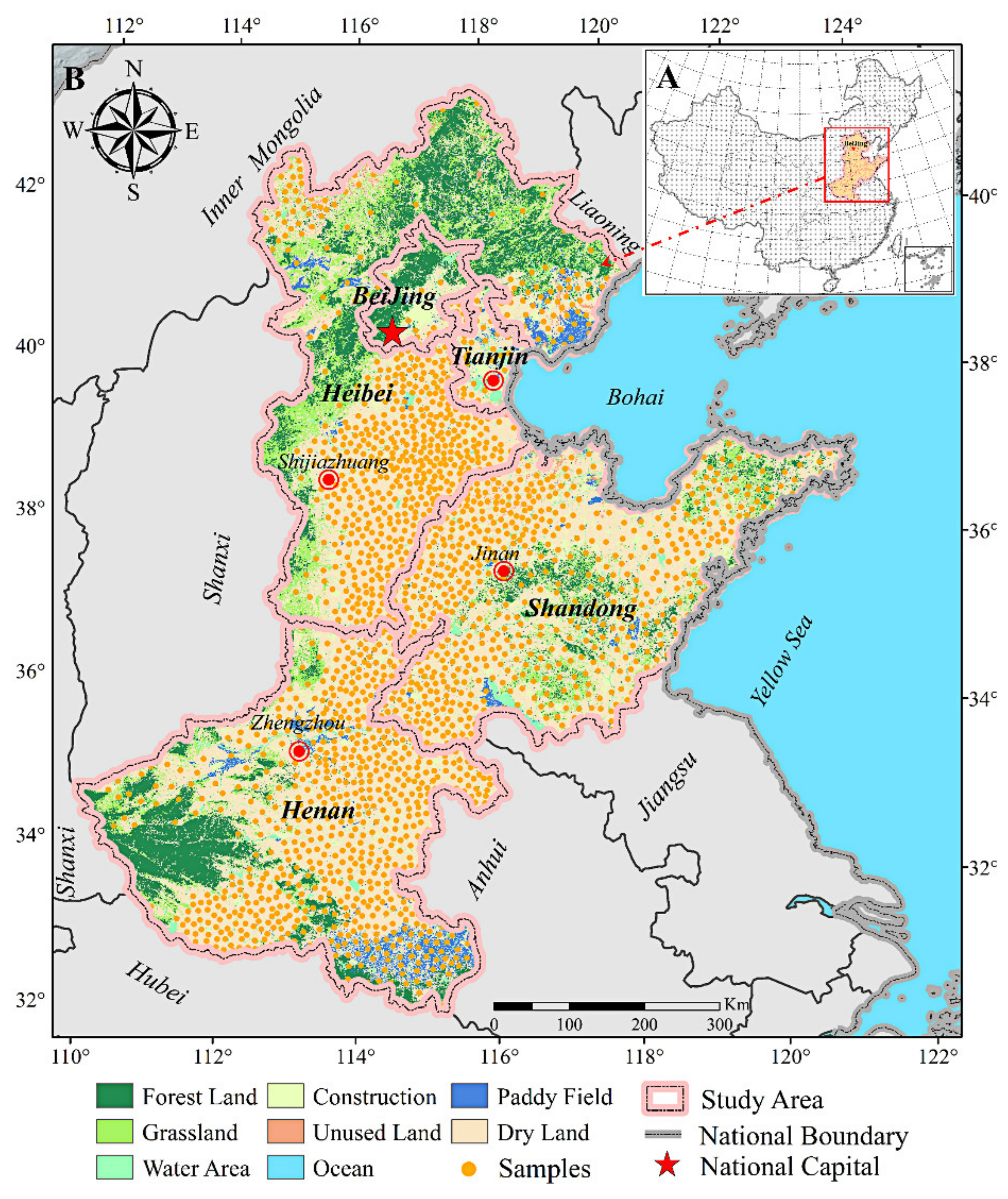
Figure 2.
Diagram showing the processes used to determine the CI of cultivated land.

Figure 3.
Smoothness of LAI time series for different cropping systems. (A) No-peak curve in fallow field; (B) unimodal curve in single cropping; (C) bimodal curve in double cropping; (D) three-peak curve in triple cropping.
Figure 3.
Smoothness of LAI time series for different cropping systems. (A) No-peak curve in fallow field; (B) unimodal curve in single cropping; (C) bimodal curve in double cropping; (D) three-peak curve in triple cropping.
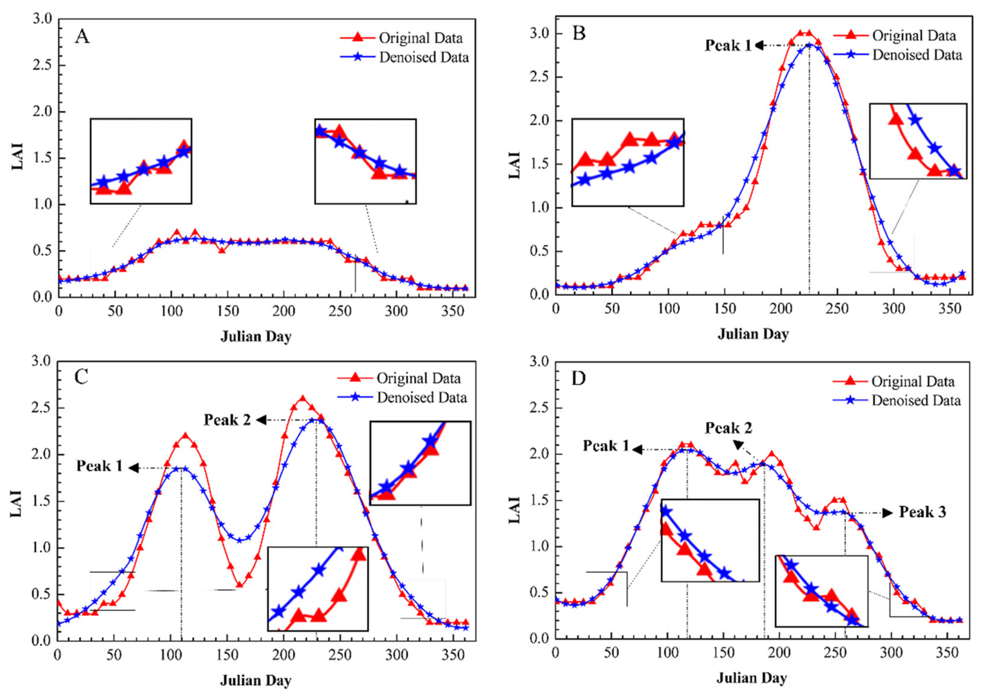
Figure 4.
Original LAI time series together with results of processing during the different steps of the second-order difference algorithm. (A) Original smoothed LAI curve; (B) result of sequence S(1); (C) result of sequence S(2); (D) result of sequence S(3).
Figure 4.
Original LAI time series together with results of processing during the different steps of the second-order difference algorithm. (A) Original smoothed LAI curve; (B) result of sequence S(1); (C) result of sequence S(2); (D) result of sequence S(3).
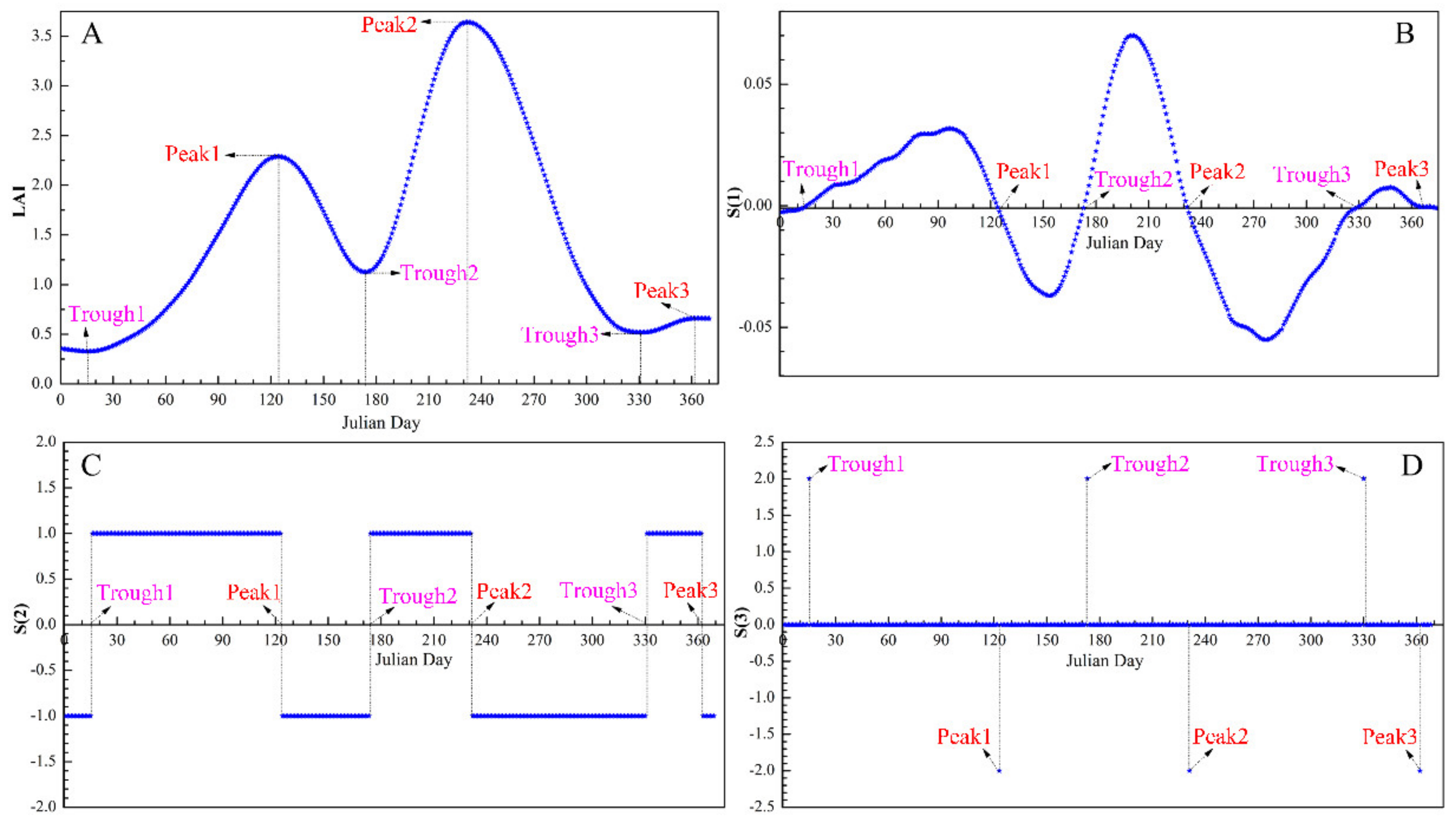
Figure 5.
Assessment of the extraction accuracy of the MCIs using a comparison with statistical data for the NCP from 1982 to 2018.
Figure 5.
Assessment of the extraction accuracy of the MCIs using a comparison with statistical data for the NCP from 1982 to 2018.
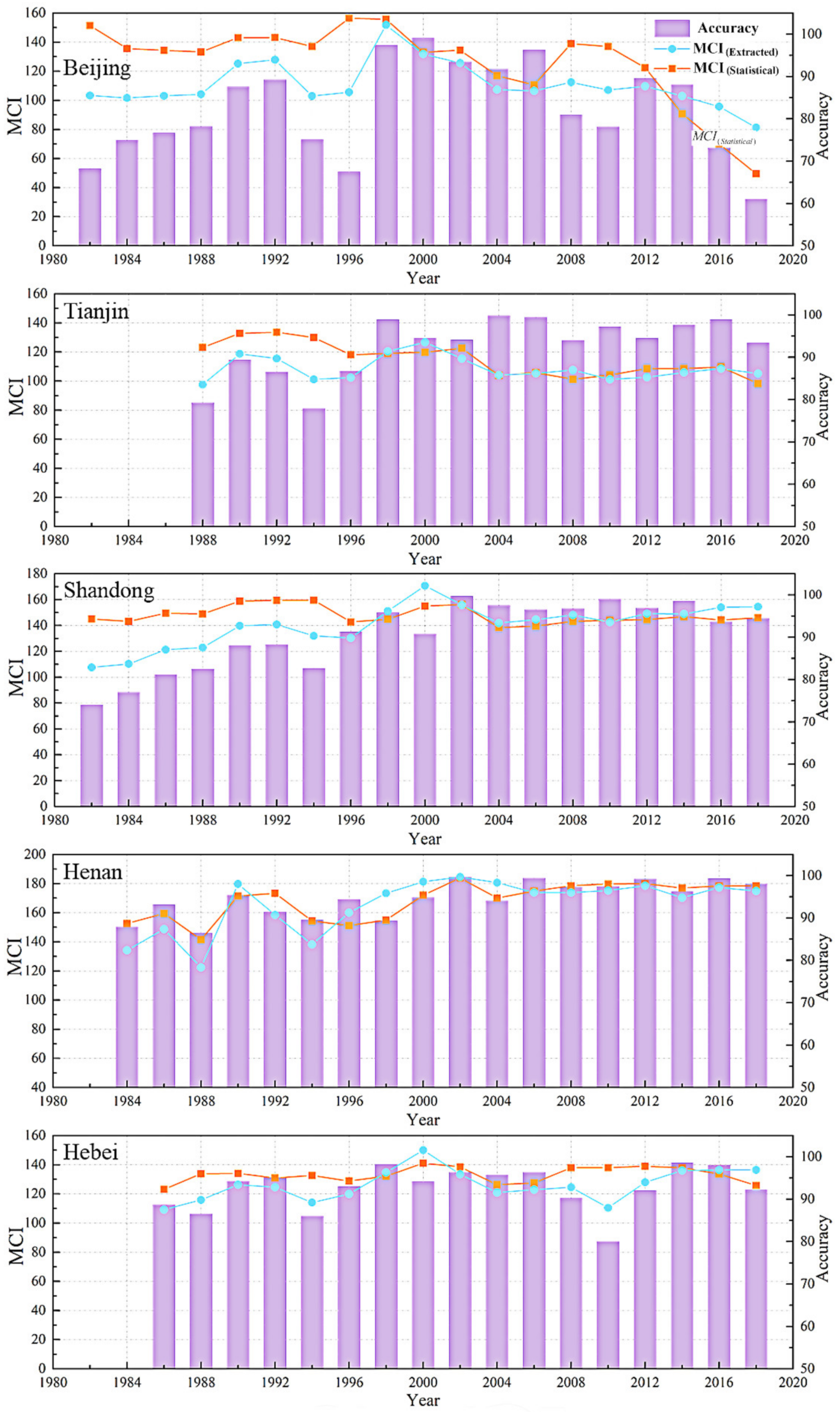
Figure 6.
Comparative analysis between the results of this study and other research results.

Figure 7.
Spatial distribution of MCI of cultivated land on the NCP from 1982 to 2018.
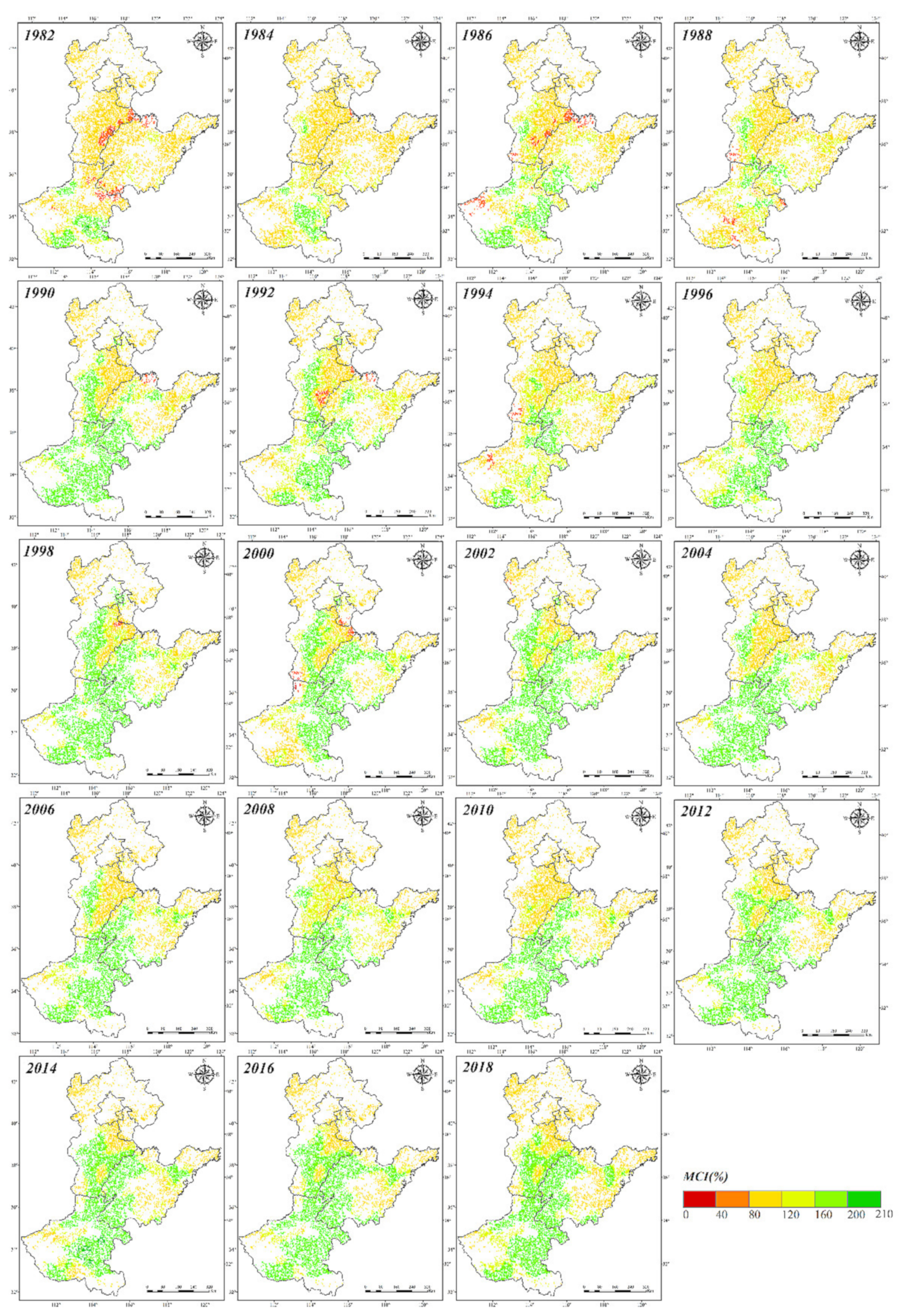
Figure 8.
The distribution pattern of the average MCI of cultivated land from 1982 to 2018, which includes the distribution for the NCP from 1982 to 2018 and the average CI of cultivated land for the 5 provinces and cities in the study area from 1982 to 2018.
Figure 8.
The distribution pattern of the average MCI of cultivated land from 1982 to 2018, which includes the distribution for the NCP from 1982 to 2018 and the average CI of cultivated land for the 5 provinces and cities in the study area from 1982 to 2018.

Figure 9.
Spatial patterns of cropping systems used on the NCP from 1982 to 2018.

Figure 10.
Interannual variation in the CI of cultivated land on the NCP and the five provinces and cities in the study area from 1982 to 2018. (A) Interannual variation in the CI of cultivated land from 1982 to 2018; (B) radar map of the interannual variation for the five provinces and cities.
Figure 10.
Interannual variation in the CI of cultivated land on the NCP and the five provinces and cities in the study area from 1982 to 2018. (A) Interannual variation in the CI of cultivated land from 1982 to 2018; (B) radar map of the interannual variation for the five provinces and cities.

Figure 11.
Annual variation in the CI on the NCP and in the different provinces and cities over different time periods.
Figure 11.
Annual variation in the CI on the NCP and in the different provinces and cities over different time periods.

Figure 12.
Percentage areas of cultivated land where different cropping systems were used on the NCP from 1982 to 2018.
Figure 12.
Percentage areas of cultivated land where different cropping systems were used on the NCP from 1982 to 2018.

Figure 13.
Comparison of GLASS LAI, AVHRR NDVI and MODIS NDVI time series curves for the NCP. (A) and (B) are the comparisons of GLASS LAI and AVHRR NDVI time series for the NCP in 1982. (C) and (D) are the comparisons of GLASS LAI and MODIS NDVI time series for the NCP in 2012.
Figure 13.
Comparison of GLASS LAI, AVHRR NDVI and MODIS NDVI time series curves for the NCP. (A) and (B) are the comparisons of GLASS LAI and AVHRR NDVI time series for the NCP in 1982. (C) and (D) are the comparisons of GLASS LAI and MODIS NDVI time series for the NCP in 2012.
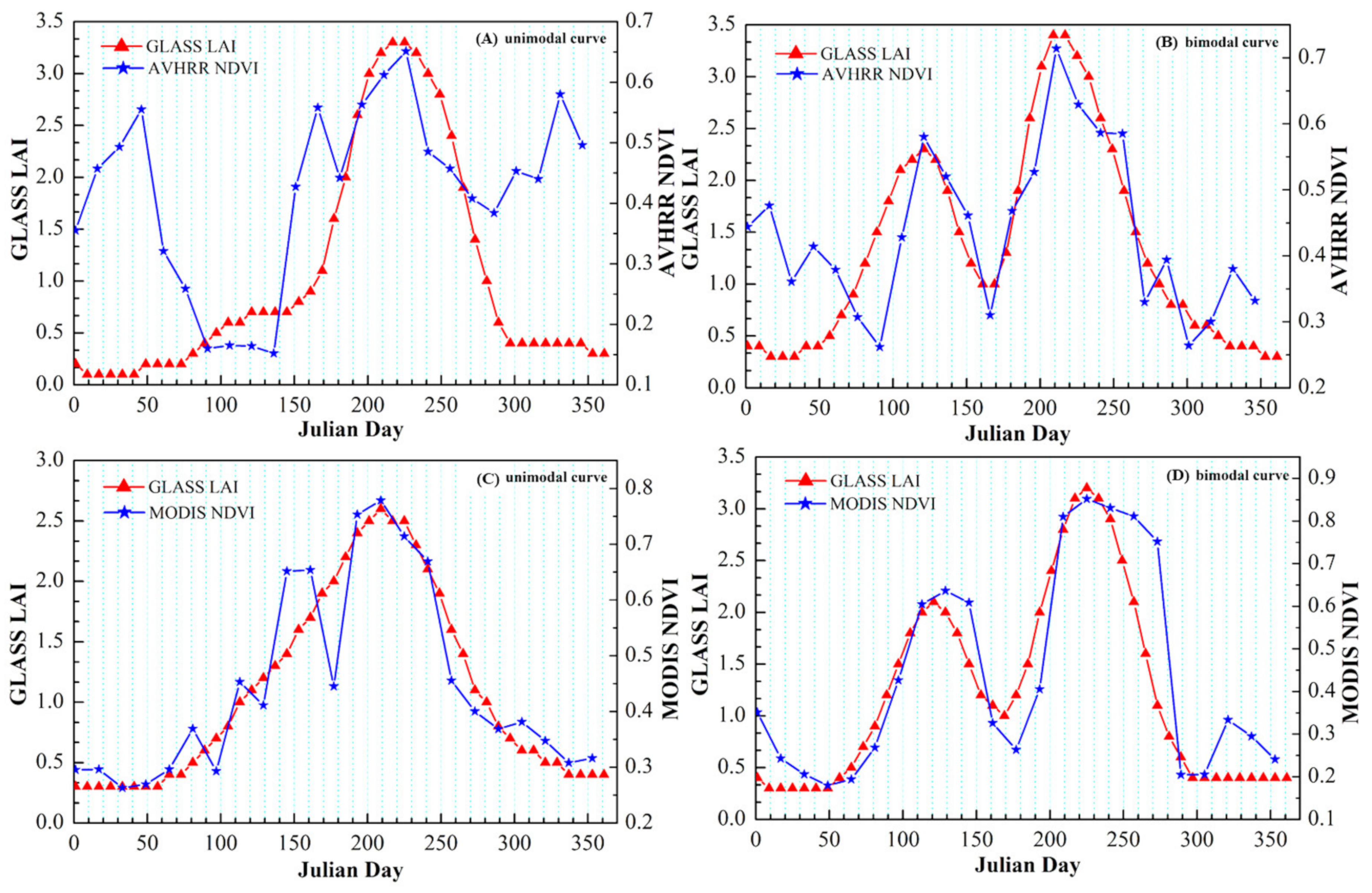
Figure 14.
Frequency distribution of the SCS and DCS cropping systems at different latitudes on the NCP from 1982 to 2018.
Figure 14.
Frequency distribution of the SCS and DCS cropping systems at different latitudes on the NCP from 1982 to 2018.

Figure 15.
Location of the northern limit of the double cropping system on the NCP from 1982 to 2018.
Figure 15.
Location of the northern limit of the double cropping system on the NCP from 1982 to 2018.


Table 1.
List of all the LAI data used in this study.
| Data Type | Dataset | Sensor | Format | Spatial Projection | Time Range | Temporal Resolution | Spatial Resolution |
|---|---|---|---|---|---|---|---|
| GLASS LAI | GLASS LAI (1982–2000) | AVHRR | HDF-EOS | geographic projection | 1982–2000 | 8 days | 0.05° |
| GLASS LAI (2001–2016) | MODIS | HDF-EOS | Integrated Sinusoidal projection | 2001–2016 | 8 days | 0.05°, 1 km, 500 m |
Table 2.
Cross-validation error matrix for the cropping systems used on the NCP.
| Interpolation Results | Extraction Results | ||||
|---|---|---|---|---|---|
| Fallow Field | SCS | DCS | Total | User Accuracy | |
| Fallow Field | 13 | 20 | 10 | 43 | 30.23% |
| SCS | 0 | 856 | 285 | 1141 | 75.02% |
| DCS | 0 | 64 | 842 | 906 | 92.94% |
| Total | 13 | 940 | 1137 | 2090 | -- |
| Producer Accuracy | 100% | 91.06% | 74.05% | -- | -- |
| Overall Accuracy = 81.87% | |||||
| Kappa Coefficient = 0.65 | |||||
Publisher’s Note: MDPI stays neutral with regard to jurisdictional claims in published maps and institutional affiliations. |
© 2021 by the authors. Licensee MDPI, Basel, Switzerland. This article is an open access article distributed under the terms and conditions of the Creative Commons Attribution (CC BY) license (https://creativecommons.org/licenses/by/4.0/).
Share and Cite
MDPI and ACS Style
Zhao, Y.; Feng, J.; Luo, L.; Bai, L.; Wan, H.; Ren, H. Monitoring Cropping Intensity Dynamics across the North China Plain from 1982 to 2018 Using GLASS LAI Products. Remote Sens. 2021, 13, 3911. https://doi.org/10.3390/rs13193911
AMA Style
Zhao Y, Feng J, Luo L, Bai L, Wan H, Ren H. Monitoring Cropping Intensity Dynamics across the North China Plain from 1982 to 2018 Using GLASS LAI Products. Remote Sensing. 2021; 13(19):3911. https://doi.org/10.3390/rs13193911
Chicago/Turabian StyleZhao, Yan, Jianzhong Feng, Lei Luo, Linyan Bai, Hong Wan, and Hongge Ren. 2021. "Monitoring Cropping Intensity Dynamics across the North China Plain from 1982 to 2018 Using GLASS LAI Products" Remote Sensing 13, no. 19: 3911. https://doi.org/10.3390/rs13193911
Note that from the first issue of 2016, this journal uses article numbers instead of page numbers. See further details here.