Estimation of Inter-System Biases between BDS-3/GPS/Galileo and Its Application in RTK Positioning

Abstract

For the development of a global navigation satellite system (GNSS), the third generation of BeiDou Navigation Satellite System (BDS-3) achieved full constellation for worldwide service on 23 June 2020. The new signals, B1C and B2a of BDS-3, further enhance the compatibility and interoperability between different GNSSs. In this study, we first assessed the quality of all the signals in BDS-3/GPS/Galileo. Then, to achieve the interoperability among BDS-3/GPS/Galileo, the inter-system bias (ISB), which appears if an inter-system difference exists between two GNSSs, was estimated at overlapping frequencies. Finally, we used the estimated ISBs in real-time kinematic (RTK) positioning. The results show the higher quality of the overlapping frequency B2a/L5/E5a than B1C/L1/E1 in terms of pseudo range multipath. The ISBs are stable both in the short term for one day and in the long term for over a year, which fit a zero-mean normal distribution well when the identical type of receiver is applied. Thus, it is reasonable to ignore the ISBs in the inter-system differences. With the estimated ISBs, the inter-system double-difference RTK can be achieved, which is called a tightly combined model (TCM) RTK. Compared with the traditional intra-system double-difference RTK, which is called a loosely combined model (LCM) RTK, the TCM RTK can achieve a higher success rate (SR) in terms of ambiguity resolution and higher positioning accuracy. In addition, the higher the cutoff elevation angle set, the greater the promotion can be obtained in SR. Even with a cutoff elevation angle of 50°, the SR of TCM is over 80%. Thus, it is important to apply TCM RTK when the observation conditions are limited, such as in dense jungles or the urban canyons.

1. Introduction

The advent of modernized global positioning system (GPS), the Galileo satellite navigation system (Galileo), and BeiDou Navigation Satellite System (BDS) have provided vital improvements in the accuracy and robustness of satellite-based positioning, navigation, and timing (PNT) service applications [1]. Having provided PNT service in the Asia-Pacific region for six years, the China Satellite Navigation Office (CSNO) officially announced that the third generation of BDS (BDS-3) began to provide global service on 27 December 2018, which was a milestone as BDS enlarged the service region from Asia-Pacific to worldwide [2,3,4]. On 13 July 2020, the chairperson of China announced the official start of BDS-3, which provides a variety of services. Specifically, it provides the PNT, global short message communication, and international search and rescue services for global users; satellite-based augmentation, ground augmentation, precise point positioning (PPP), and regional short message communication services can be obtained throughout China [5]. As designed, the constellation of BDS-3 consists of 3 geostationary orbit (GEO) satellites, 3 inclined geo-synchronous orbit (IGSO) satellites, and 24 medium Earth orbit (MEO) satellites [6]. Yang [7] comprehensively introduced BDS-3 in terms of its constellation, signal, service, etc. Zhang [6] assessed the system status and positioning performance of BDS-2/3 with large amounts of observation data distributed around the globe. The new signals of BDS-3 were initially assessed by Zhang [8] from various aspects: its constellation, signal quality, and the accuracy of relative positioning with combined BDS-2/3. As for other GNSSs, the new generation of GPS III-A is gradually updating and a total of 31 operational satellites comprise the GPS constellation [9], whereas 26 satellites can be tracked in the Galileo constellation [10].

As a typical technology of relative positioning, real-time kinematic (RTK) positioning is widely applied in marine navigation, velocity measurements, automatic driving, etc. [11,12,13]. Centimeter-level precision can be achieved when the float ambiguities are correctly fixed to integers [14]. In the functional RTK model, various observational errors are eliminated by the double difference (DD). Specifically, the satellite-based and receiver-based observational errors are eliminated by between-receiver single difference (SD) and between-satellite SD, respectively [15]. In the DD observations, most of the atmosphere delay can be eliminated considering the short distance between the base station and the rover station [16]. In the past, extensive research on the single GPS RTK was conducted to evaluate its performance in different situations [17,18,19]. The application of single GPS RTK may be extremely limited due to the insufficient number of satellites and the poor configuration of the constellation in hostile environments. However, with the rapid development of GNSSs, the multi-system RTK has become accessible and the application scope of RTK was further broadened [20,21,22]. In multi-system RTK, not only the vital ambiguity resolution, but also the accuracy and reliability of positioning results are improved remarkably compared to the single-system RTK. Li [23] analyzed the performance of GPS + BDS RTK and found that the success rate (SR) and reliability of GPS + BDS RTK are better than those of GPS in instantaneous RTK. Teunissen [22] reported that, with the combined system of GPS + BDS, much larger (40°) cutoff elevations than the customary value (10°) can be used in RTK positioning. Odolinski [20] compared single-frequency dual-system (SF-DS) RTK with dual-frequency single-system (DF-SS) RTK in single-epoch mode, and the results showed that low-cost receivers for SF-DSs have the potential to achieve comparable ambiguity resolution performance to that of a DF-SS. The above studies were conducted by considering different GNSSs separately, which is called the loosely combined model (LCM) of RTK since each GNSS needs a pivot satellite.

Benefitting from the overlapping frequency, the compatibility and interoperability between various systems have become accessible. Odijk [24,25] introduced the theory of inter-system bias (ISB) and found the ISB between GPS and Galileo was stable over time when their overlapping frequency observations are applied in the inter-system DD equation. In Odolinski [26], the ISB between GPS and the Japanese Quasi Zenith Satellite System (QZSS) was evaluated as being so stable that the ISB can be safely neglected to maximize the redundancy of multi-system RTK. Mi [27] compared the ISBs between BDS-3, GPS, and Galileo, and proved the interoperability between these GNSSs. Wu [28] analyzed the ISB between GPS and BDS-3/Galileo with the overlapping frequency. The results indicated that when identical receiver types were applied, the ISBs were close to zero. In contrast, the ISB generally exists but is stable when different types of receivers were applied. The above research provides evidence that ISBs exist in inter-system difference observations, and the stability of ISB enables their calibration. After correcting the ISB in the inter-system difference observations, the tightly combined model (TCM) of RTK is established, which shares a common pivot satellite between overlapping frequencies.

In this article, we first analyze the quality of the signals transmitted by BDS-3, GPS, and Galileo in terms of the noise level of both pseudo range and phase observations. Then, with many observations, we extract the ISBs of BDS-3, GPS, and Galileo at overlapping frequency to verify their short- and long-term stability. Afterwards, the positioning performance of single-system and multi-system RTK is analyzed in terms of positioning errors and SR. Finally, with the extracted ISBs, the performance of the multi-system TCM RTK is evaluated with different cutoff elevation angles in contrast to LCM RTK.

2. RTK Positioning Models

In this section, the function models of LCM RTK and TCM RTK together with ISB estimation are derived after the introduction of the GNSS observations. Then, the stochastic model of both the RTK and ISB model is demonstrated.

2.1. GNSS Observations

The range measurements of GNSS mainly include the phase and code observations. If the receiver $r$ is tracking satellites $s_{*}=1_{*},\hspace{0.33em}{2}_{*},\hspace{0.33em}\cdots ,\hspace{0.33em}{n}_{*}$, where $n$ is the number of satellites of a single GNSS $\ast$, such as BDS3, GPS, and Galileo, then the multi-frequency GNSS observations can be given by [15]:

$$\begin{array}{l}{\varphi }_{r,f}^{s_{*}}={\rho }_r^{s_{*}}+d{t}_r-d{t}^{s_{*}}-i_{r,f}^{s_{\ast }}+t_r+\lambda (a_r^{s_{*}}+{\delta }_{r,f}^{\ast }-{\delta }_f^{s_{*}}+{\phi }_{r,f}-{\phi }_f^{s_{*}})+d{t}_{TO}^{\ast }+{\epsilon }_{r,f}^{s_{*}}\\ P_{r,f}^{s_{*}}={\rho }_r^{s_{*}}+d{t}_r-d{t}^{s_{*}}+i_{r,f}^{s_{\ast }}+t_r+d_{r,f}^{\ast }-d_f^{s_{*}}+d{t}_{TO}^{\ast }+e_{r,f}^{s_{*}}\end{array}$$

(1)

where $\varphi$ and $P$ denote the phase and code observations, respectively; $\rho$ is the geometric distance between the satellite and the receiver; $d{t}_r$ and $d{t}^{s_{*}}$ are the clock bias in the receiver and satellite, respectively; $i$ and $t$ are the ionospheric and tropospheric delay, respectively; $\lambda$ is the wavelength of frequency $f$; $a$ denotes the unknown ambiguity; ${\delta }_{r,f}^{\ast }$ and ${\delta }_f^{s_{*}}$ denote the phase hardware delay in the receiver and satellite, respectively; $d_{r,f}^{\ast }$ and $d_f^{s_{*}}$ denote the code hardware delay in the receiver and satellite, respectively; ${\phi }_{r,f}$ and ${\phi }_f^{s_{*}}$ are the initial phase biases in the receiver and satellite; ${\epsilon }_{r,f}^{s_{*}}$ and $e_{r,f}^{s_{*}}$ are the noise of the phase and code observations, respectively; and $d{t}_{TO}$ is the time offset from GPS to other GNSSs.

In this article, an elevation dependent method is applied to weight different types of observations. The empirical stochastic model can be stated as:

$${\sigma }_{\theta }=\frac{{\sigma }_0}{\sin (\theta )}$$

(2)

where ${\sigma }_{\theta }$ denotes the prior standard deviation (STD) of undifferenced observations with an elevation of $\theta$; ${\sigma }_0$ denotes the prior zenith STD for phase and code observations, which is usually set according to the accuracy of observations. In this article, the custom set of the STD of the observation noise was used, which is 0.003 m for phase observation and 0.3 m for code observation.

2.2. LCM RTK

Assuming that two receivers, rover station $r$ and base station $b$, are tracking the same satellites $s_{*}=1_{*},\hspace{0.33em}{2}_{*},\hspace{0.33em}\cdots ,\hspace{0.33em}{m}_{*}$, where $m$ is the number of the common-view satellites of a single GNSS $\ast$ (assume the $1_{*}$ as the pivot satellites), the intra-system DD observation equation of multi-system, multi-frequency can be given as:

$$\begin{array}{l}{\varphi }_{rb,f}^{1_G{s}_G}={\rho }_{rb}^{1_G{s}_G}+{\lambda }_f{a}_{rb,f}^{1_G{s}_G}+{\epsilon }_{rb,f}^{1_G{s}_G}\\ {\varphi }_{rb,f}^{1_{\ast }{s}_{\ast }}={\rho }_{rb}^{1_{\ast }{s}_{\ast }}+{\lambda }_f{a}_{rb,f}^{1_{\ast }{s}_{\ast }}+{\epsilon }_{rb,f}^{1_{\ast }{s}_{\ast }}\\ P_{rb,f}^{1_G{s}_G}={\rho }_{rb}^{1_G{s}_G}+e_{rb,f}^{1_G{s}_G}\\ P_{rb,f}^{1_{\ast }{s}_{\ast }}={\rho }_{rb}^{1_{\ast }{s}_{\ast }}+e_{rb,f}^{1_{\ast }{s}_{\ast }}\end{array}$$

(3)

where ${[·]}_{rb,f}^{1_{\ast }{s}_{\ast }}$ denotes the DD procedure ($·$ denotes different elements in Equation (3)) and $s_{\ast }$ is the satellites, except the pivot satellite $1\ast$. The delays in the receivers and satellites are eliminated completely in the process of DD. Most of the atmospheric delays can be eliminated, so we ignore the influence of the atmospheric delay where there are relatively short baselines in this article. However, the impact of the ionosphere on the positioning with a relatively long baseline cannot be ignored. In this case, ionospheric delays should be estimated [29,30].

In the LCM RTK function model, every GNSS needs a pivot for the difference inside the GNSS. Thus, when more GNSSs are used, more pivot satellites are needed.

2.3. ISB and TCM RTK

Different from LCM RTK, TCM RTK only needs one common pivot satellite for all the GNSS applied. However, the restriction is that only in the observation of overlapping frequency can the inter-system DD be completed. In addition, extra parameters known as code and phase ISBs appear in the inter-system DD observation. Prior estimation of the ISBs is required, which can be corrected as a constant to enhance our TCM model. To estimate the ISBs, prior position information about the receivers should be known, and then the equation to estimate ISB can be given as:

$$\begin{array}{l}{\varphi }_{rb,f}^{1_G{s}_G}={\rho }_{rb}^{1_G{s}_G}+{\lambda }_f{a}_{rb,f}^{1_G{s}_G}+{\epsilon }_{rb,f}^{1_G{s}_G}\\ {\varphi }_{rb,f}^{1_G{s}_{\ast }}={\rho }_{rb}^{1_G{s}_{\ast }}+{\lambda }_f(a_{rb,f}^{1_G{s}_{\ast }}+{\delta }_{rb,f}^{G\ast })+{\epsilon }_{rb,f}^{1_G{s}_{\ast }}\\ P_{rb,f}^{1_G{s}_G}={\rho }_{rb}^{1_G{s}_G}+e_{rb,f}^{1_G{s}_G}\\ P_{rb,f}^{1_G{s}_{\ast }}={\rho }_{rb}^{1_G{s}_{\ast }}+d_{rb,f}^{G\ast }+e_{rb,f}^{1_G{s}_{\ast }}\end{array}$$

(4)

where ${\delta }_{rb,f}^{G\ast }$ and $d_{rb,f}^{G\ast }$ denote the code and phase ISB, respectively. In Equation (4), there is a rank deficiency between the vector of ambiguities and the phase ISB. To solve this rank deficiency and make the equations solvable, the usual method is to fix the phase ISB to one float ambiguity. By choosing $1\ast$ as the satellite to absorb phase ISB, the estimable form of Equation (4) is:

$$\begin{array}{l}{\varphi }_{rb,f}^{1_G{s}_G}={\rho }_{rb}^{1_G{s}_G}+{\lambda }_f{a}_{rb,f}^{1_G{s}_G}+{\epsilon }_{rb,f}^{1_G{s}_G}\\ {\varphi }_{rb,f}^{1_G{s}_{\ast }}={\rho }_{rb}^{1_G{s}_{\ast }}+{\lambda }_f(a_{rb,f}^{1_{\ast }{s}_{\ast }}+{\overline{\delta }}_{rb,f}^{G\ast })+{\epsilon }_{rb,f}^{1_G{s}_{\ast }}\\ P_{rb,f}^{1_G{s}_G}={\rho }_{rb}^{1_G{s}_G}+e_{rb,f}^{1_G{s}_G}\\ P_{rb,f}^{1_G{s}_{\ast }}={\rho }_{rb}^{1_G{s}_{\ast }}+d_{rb,f}^{G\ast }+e_{rb,f}^{1_G{s}_{\ast }}\end{array}$$

(5)

where ${\overline{\delta }}_{rb,f}^{G\ast }={\delta }_{rb,f}^{G\ast }+a_{rb,f}^{1_G{1}_{*}}$ denotes the float ambiguity that absorbs the phase ISB. After the estimation of Equation (5), the phase ISB can be extracted through integer rounding:

$${\widehat{\delta }}_{rb,f}^{G\ast }={\overline{\delta }}_{rb,f}^{G\ast }-Round({\overline{\delta }}_{rb,f}^{G\ast })$$

(6)

where $Round(·)$ denotes the integer rounding and ${\widehat{\delta }}_{rb,f}^{G\ast }$ is the estimation of phase ISB that needs to be corrected in the inter-system DD observation.

Now, with the estimated ISBs, the inter-system DD can be conducted with the ISB corrected as:

$$\begin{array}{l}{\varphi }_{rb,f}^{1_G{s}_G}={\rho }_{rb}^{1_G{s}_G}+{\lambda }_f{a}_{rb,f}^{1_G{s}_G}+{\epsilon }_{rb,f}^{1_G{s}_G}\\ {\overline{\varphi }}_{rb,f}^{1_G{s}_{\ast }}={\rho }_{rb}^{1_G{s}_{\ast }}+{\lambda }_f{a}_{rb,f}^{1_G{s}_{\ast }}+{\epsilon }_{rb,f}^{1_G{s}_{\ast }}\\ P_{rb,f}^{1_G{s}_G}={\rho }_{rb}^{1_G{s}_G}+e_{rb,f}^{1_G{s}_G}\\ {\overline{P}}_{rb,f}^{1_G{s}_{\ast }}={\rho }_{rb}^{1_G{s}_{\ast }}+e_{rb,f}^{1_G{s}_{\ast }}\end{array}$$

(7)

where ${\overline{\varphi }}_{rb,f}^{1_G{s}_{\ast }}={\varphi }_{rb,f}^{1_G{s}_{\ast }}-{\lambda }_f{\widehat{\delta }}_{rb,f}^{G\ast }$ and ${\overline{P}}_{rb,f}^{1_G{s}_{\ast }}{=\mathrm{P}}_{rb,f}^{1_G{s}_{\ast }}-d_{rb,f}^{G\ast }$ denotes the inter-system DD observation with phase and code ISBs corrected, respectively; $1_G$ is the unique pivot satellite for all the GNSSs; and $s_{*}$ represents BDS-3/GPS/Galileo satellite. In the inter-system DD observations, the ISBs should be calibrated in advance and then be corrected so the stability of ISBs can be assured. Specifically, the ISBs between the two systems (BDS-3/GPS/Galileo system) should be corrected in the inter-system DD observations by subtracting the calibrated ISBs. Then, the ambiguity of the inter-system DD obtains its integer nature and can be fixed by LAMBDA [31]. Thus, for each two overlapping frequencies in two different GNSSs, an extra redundant observation can be obtained, which improves the RTK function model.

Table 1. Frequency and wavelength of BDS-3/GPS/Galileo.

Frequency (MHz)	Wavelength (cm)	BDS-3	GPS	Galileo
1575.42	19.03	B1C	L1	E1
1561.098	19.20	B1I	-	-
1278.75	23.44	-	-	E6
1268.52	23.63	B3I	-	-
1227.60	24.42	-	L2	-
1207.14	24.83	B2b	-	E5b
1191.795	25.15	-	-	E5
1176.45	25.48	B2a	L5	E5a

shows the frequency and wavelength of BDS-3/GPS/Galileo. It can be observed that B1C, L1, and E1 share the same frequency, 1575.42 MHz, whereas B2a, L5, and E5a share the same frequency, 1176.45 MHz, among BDS-3, GPS, and Galileo.

3. Datasets and Experiments

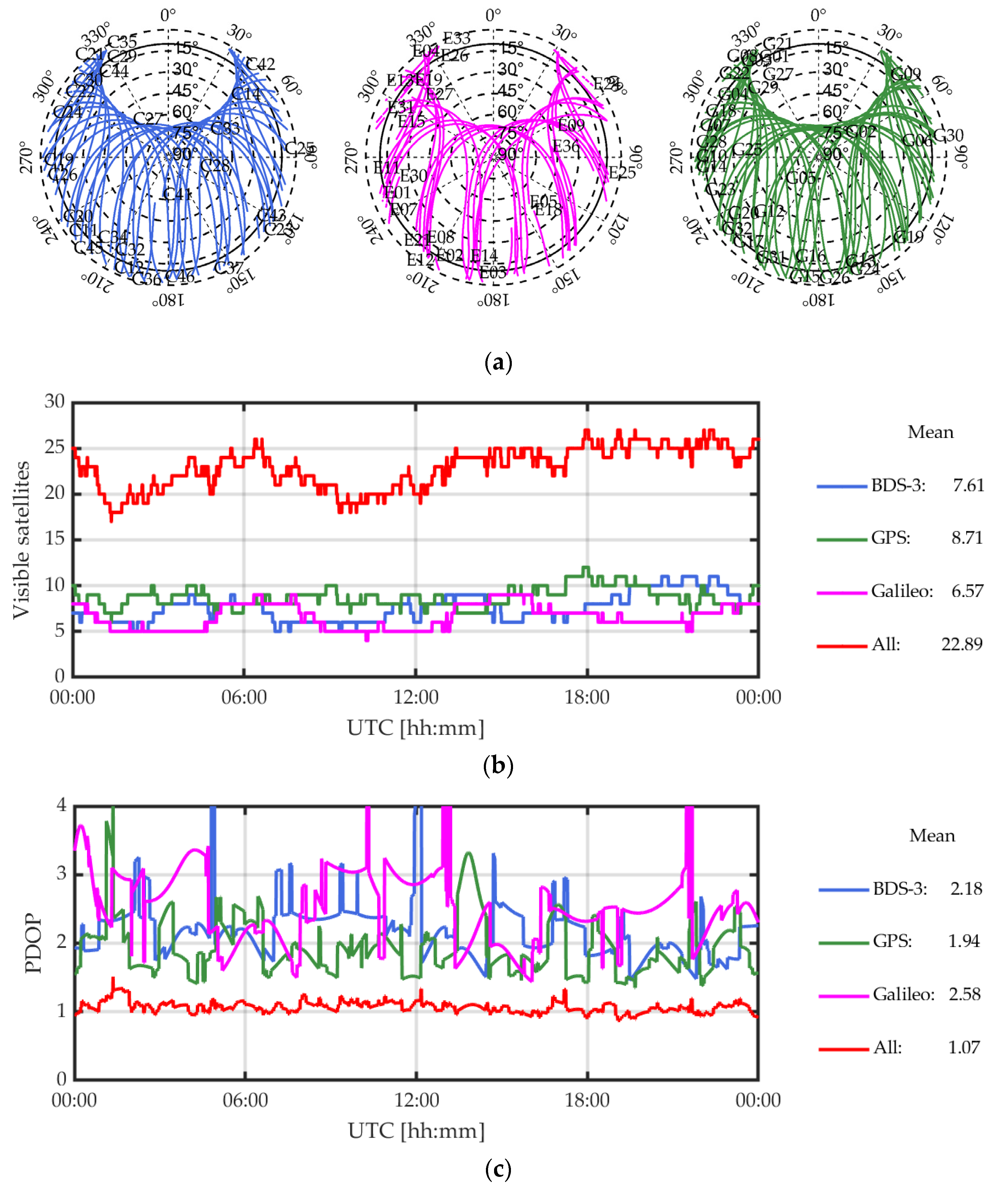
In this section, we firstly introduce the information about the datasets, including the information about the receivers and antennas, the position of the stations, the visible satellites of different GNSSs, etc. We then describe some analyses of the quality of different signals in terms of the pseudo range multipath and the noise of phase observation. Finally, the stability of ISB between overlapping frequencies and the performance of single-system, multi-system LCM RTK, and TCM RTK is analyzed.

3.1. Datasets

The datasets used in this article were obtained from four different stations from the International GNSS Service (IGS). To describe the information of the stations,

Table 2. Information of experimental datasets for all the receivers.

Station	Location	Receiver	Antenna	Longitude	Latitude
GODN 1	America	JAVAD TRE_3 DELTA	TPSCR.G3	${39}^{\circ }{1}^{\prime }16^{″}$	$-{76}^{\circ }49^{\prime }38^{″}$
GODS 1	America	JAVAD TRE_3 DELTA	JAVRINGANT_DM	${39}^{\circ }{1}^{\prime }14^{″}$	$-{76}^{\circ }49^{\prime }38^{″}$
GODE 2	America	SEPT POLARX5TR	AOAD/M_T	${39}^{\circ }{1}^{\prime }18^{″}$	$-{76}^{\circ }49^{\prime }37^{″}$
USN7 2	America	SEPT POLARX5TR	TPSCR.G5	${38}^{\circ }55^{\prime }14^{″}$	$-{76}^{\circ }{3}^{\prime }59^{″}$

¹ The duration of the station GODN and GODS is from day-of-year (DOY) 29, 2020 to DOY 150, 2021. ² The duration of the station GODE and USN7 is from DOY 36, 2021 to DOY 150, 2021.

shows the location, position, and other information of the receivers. Station GODN is in the middle between GODS and GODE, which consists of one baseline, GODN-GODS, with the identical-receiver type of 65.16 m, and one baseline, GODN-GODE, with a different-receiver type of 76.02 m. Station USN7 forms a baseline of medium length of about 22.82 km with GODE. All the data were collected at a sampling interval of 30 s.

In addition to the information about the stations, the visibility of satellites is equally important. The top of Figure 1 displays the sky plots of BDS-3, GPS, and Galileo. Due to the location restrictions, none of the IGSO or GEO satellites of BDS-3 can be tracked. The observed satellites include 24 BDS-3, 31 GPS, and 24 Galileo satellites. In addition, only 16 GPS satellites can transmit signals in the L5 band. The middle of Figure 1 depicts the time-series of the visible satellites of different GNSSs with a cutoff elevation angle of 10°. The legend shows that the average number of visible satellites in BDS-3, GPS, and Galileo is 7.61, 8.71, and 6.57, respectively. The average number of visible satellites with a high cutoff elevation angle of 40° is 3.58, 3.90, and 3.23 satellites for BDS-3, GPS, and Galileo, respectively. To evaluate the configuration of the constellation, the position dilution of precision (PDOP) of different GNSS was introduced. The PDOP reflects not only the number of satellites, but also the performance of the distribution of the constellation. Generally, a constellation with a PDOP lower than 3.0 is regarded as having a good distribution [6,32]. The time series of PDOP of BDS-3, GPS, Galileo, and triple-system combined constellation are shown in the bottom of Figure 1. With the largest number of visible satellites, the BDS-3/GPS/Galileo combined constellation corresponds has the lowest PDOP of 1.07. As for the single systems, the average PDOP of BDS-3, GPS, and Galileo is 2.18, 1.94, and 2.58, respectively.

3.2. Quality of the Signals

3.2.1. Multipath Errors for Pseudo Range

As a linear combined observation, the pseudo range multipath (MP) combination can reflect the quality of pseudo range observations and observation environments through its noise level, which is defined as [33]:

$$M{P}_i=p_i-\frac{f_i^2+f_j^2}{f_i^2-f_j^2}{\varphi }_i+\frac{2f_j^2}{f_i^2-f_j^2}{\varphi }_j$$

(8)

where $M{P}_i$ denotes the pseudo range MP of the frequency $i$; the subscript $i$, $j$ denotes different frequency.

In the pseudo range MP combination, the atmosphere delays and geometry-based parameters are eliminated by the MP linear combination such that the remaining part of the MP combination contains the linear combination of the phase ambiguities, hardware delays, as well as multipath effects. When no cycle slip occurs, the ambiguity and the hardware delay are considered a constant and can be calculated by averaging over epochs. Thus, a subsection mean method [8] can be applied to extract the residuals of the MP combination, which are mainly influenced by the pseudo range MP in the continuous tracking of signals.

By extracting the residual MP, we compute the root mean square (RMS) of the MP for different signals with an elevation interval of 2°. Figure 2 plots the RMS of MP vs. elevation of all the signals in BDS-3, GPS, and Galileo. It is apparent that the RMS of MP decreases as the elevation increases, which indicates that the quality of signals may be higher at high elevation. For specific comparison, in BDS-3, the highest RMS of MP occurs in B1I, whose value is over 0.8 m at low elevation and over 0.2 m at an elevation higher than 80°. B2a and B3I perform similarly, whereas B2b received the lowest RMS of MP. Despite B1C has the higher RMS of MP of B2a, B2b, and B3I, it performs better than B1I, whose RMS of MP varies from about 0.45 m (at an elevation of 10°) to about 0.15 m (near the zenith). In GPS, the RMS of MP in L2 decreases fast from about 0.78 to 0.1 m with increasing elevation. L5 receives a lower RMS of MP than L1 over all elevations. In Galileo, the order of the values of the RMS of the MP in different signals is E5b, E5, E5a, E1, and E6. By comparing the RMS of the MP in different signals, we found that the overlapping frequency B2a/L5/E5a corresponds to a lower RMS value of MP than B1C/L1/E1 in BDS-3, GPS, and Galileo over all elevations.

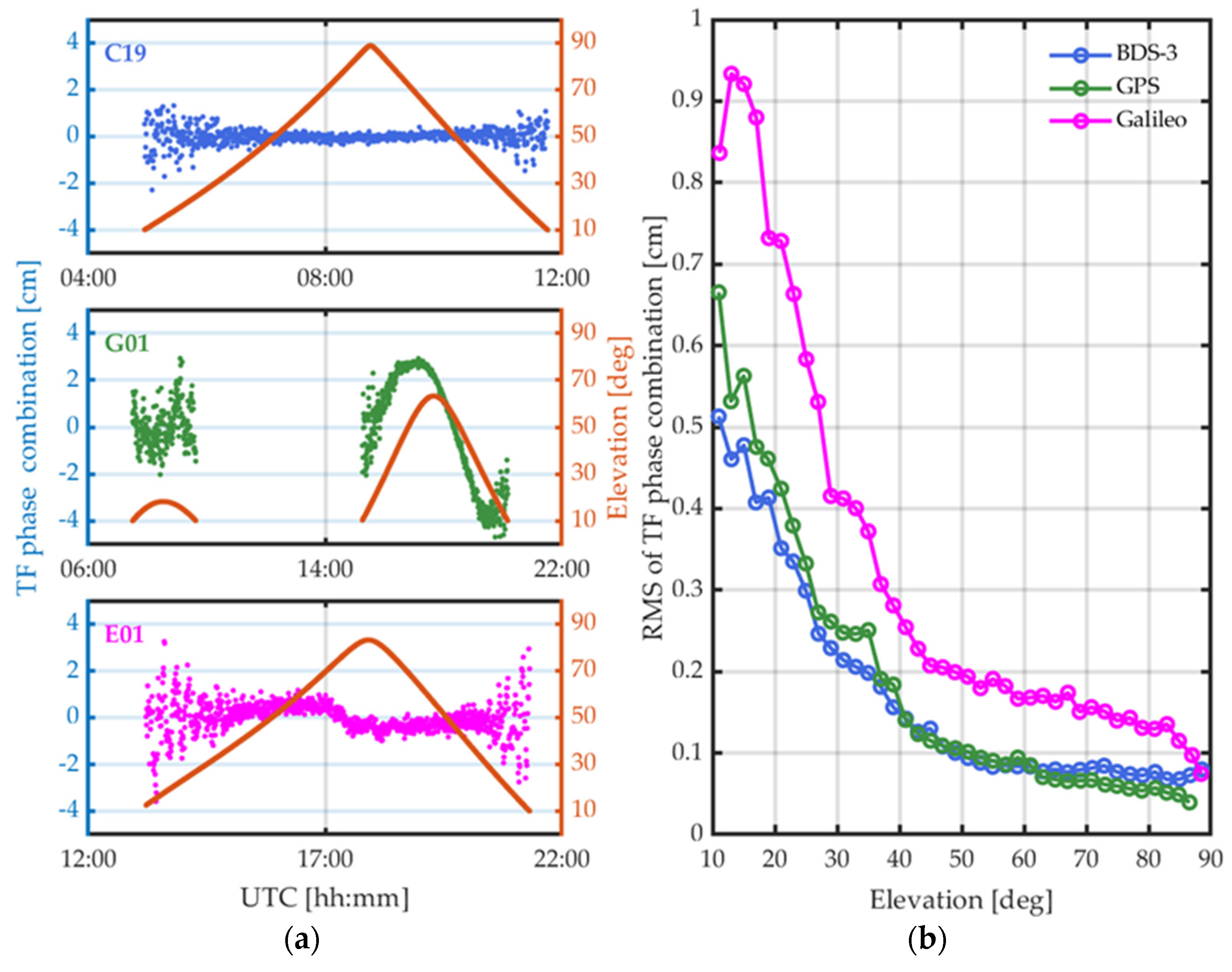
3.2.2. Triple-Frequency Phase Combination

The triple-frequency (TF) phase combination, which is extracted by the difference in two different ionosphere-free (IF) combinations, is available, but at least three different phase observations should exist in one satellite. Thus, the TF phase combination is both geometry-free and ionosphere-free and can be applied in the evaluation of the noise of phase observations, which is defined as [8]:

$$\begin{array}{ll}TFP& =(\frac{f_1^2}{f_1^2-f_2^2}{\varphi }_1-\frac{f_2^2}{f_1^2-f_2^2}{\varphi }_2)-(\frac{f_1^2}{f_1^2-f_3^2}{\varphi }_1-\frac{f_3^2}{f_1^2-f_3^2}{\varphi }_3)\\ & =(\frac{f_1^2}{f_1^2-f_2^2}-\frac{f_1^2}{f_1^2-f_3^2}){\varphi }_1-\frac{f_2^2}{f_1^2-f_2^2}{\varphi }_2+\frac{f_3^2}{f_1^2-f_3^2}{\varphi }_3\end{array}$$

(9)

where $TFP$ denotes the TF phase combination; $f_1$, $f_2$, and $f_3$ are the frequencies of the phase observations ${\phi }_1$, ${\phi }_2$, and ${\phi }_3$ in meters, respectively. Then, the residuals of the TF phase combination can be extracted by subtracting the mean value of the combination in the continuous observations when no cycle slips occur to eliminate the unknown ambiguity in the combination.

To compute the TF phase combination in BDS-3/GPS/Galileo,

Table 3. The choice of the frequencies used to compute triple frequency (TF) phase combinations and the corresponding coefficient and amplification factor of phase observations.

System	Signal 1 1	Signal 2 1	Signal 3 1	Amplification Factor
BDS-3	B1C (−0.1614)	B2a (−1.2606)	B2b (1.4220)	1.9071
GPS	L1 (0.2851)	L2 (−1.5457)	L5 (1.2606)	2.0149
Galileo	E1 (−0.1614)	E5a (−1.2606)	E5b (1.4220)	1.9071

¹ The decimals in the brackets denote the corresponding coefficient of the phase observation in TF phase observations.

shows the sets of the frequencies in BDS-3/GPS/Galileo. Table 3 lists the corresponding coefficients of the phase observations in TF phase combination. Influenced by these coefficients, the noise of TF phase combination is magnified with respect to any original phase observations. Thus, the amplification factor of BDS-3/GPS/Galileo in TF phase combination is also listed in Table 3.

Figure 3 displays the time series of the TF phase combination of C19, G01, and E01 in the left panel. The noise decreases as the elevation increases in C19 and E01. However, some bias variation occurs in the TF phase combination of G01, which is known as inter-frequency clock bias (IFCB) [34]. In past studies [8,35], the presence of IFCB in GPS was identified, whereas no apparent bias variation appears in Galileo or BDS-3. To eliminate this kind of bias variation, the between-receiver difference is the method usually applied because the IFCB remains the same for a certain satellite in different stations. Figure 3 displays the RMS of the between-receiver difference in the TF phase combination against the elevation for every 2° with all satellites considered. The between-receiver difference in the TF phase combination further magnifies the noise, and we only considered the amplification factor influenced by the coefficients of the phase observations. It is clear that Galileo has the largest RMS over all elevations compared to BDS-3 or GPS after IFCB correction. When the elevation is lower than 40°, BDS-3 has a lower RMS than GPS. However, with increasing elevation, the RMS of BDS-3 and GPS are at a similar level of about 0.5–1 mm. As for Galileo, the RMS remains at a high level, over 1 mm, even at a relatively high elevation.

3.3. Stability of ISBs

In this part, we analyze the distribution of both code and phase ISBs in the short and long terms. By analyzing the short term, one day, we show the time-series of the ISB between the overlapping frequencies of B1C/L1/E1 and B2a/L5/E5a in BDS-3/GPS/Galileo. Then, the stability of the ISBs is assessed using the mean value and STD. By analyzing the long term, one year, we show the distribution, probability density function (PDF) and quantile against the quantile (QQ) plot of the ISBs between different overlapping frequencies. Then, the mean value by day, the STD by day, and box plot by month are displayed for a comprehensive assessment of the stability of the ISBs. All the ISBs were calibrated based on the identical type of receiver with a cutoff elevation angle of 15°. The broadcast ephemeris was used to compute the position of satellites. Considering the relatively short length of the baseline GODN-GODS, we ignore the atmosphere delays when estimating ISBs. The noise of code and phase observations were set to 0.3 and 0.003 m, respectively.

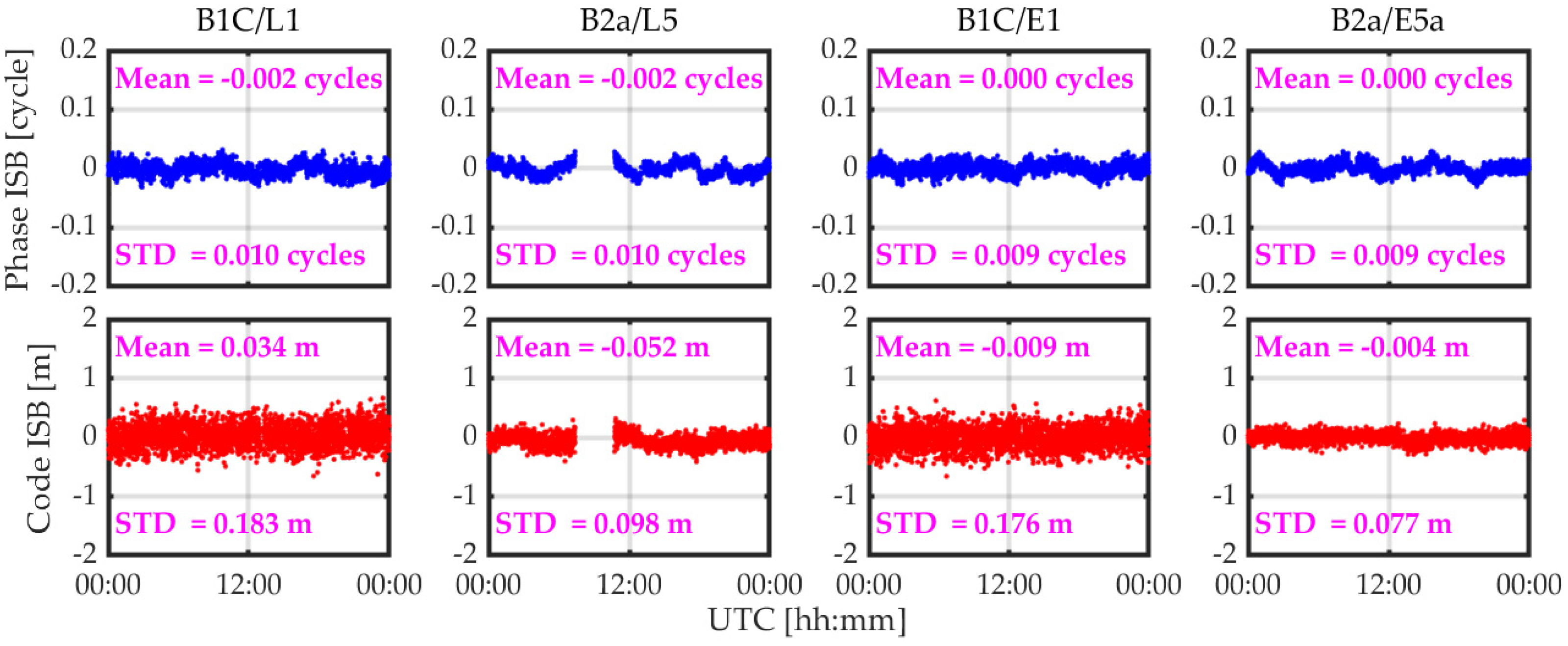
3.3.1. Short-Term ISB

As few visible GPS satellites transmit the L5 signals, we selected BDS-3 as the pivot system. The ISBs of overlapping frequencies of B1C/L1/E1 and B2a/L5/E5a in BDS-3, GPS, and Galileo were all assessed to analyze their stability.

Figure 4 displays the time series of both phase and code ISBs for the baseline GODN-GODS on DOY 120, 2021. The corresponding statistics of the short-term ISB are summarized in

Table 4. Mean value and Standard Deviation (STD) of short-term ISB.

Frequency Pair	Phase ISB (Cycle)		Code ISB (m)
	Expectation	STD	Expectation	STD
B1C/L1	−0.002	0.010	0.034	0.183
B2a/L5	−0.002	0.010	−0.052	0.098
B1C/E1	0.000	0.009	−0.009	0.176
B2a/E5a	0.000	0.009	−0.004	0.077

. Taking BDS-3 as the pivot system, all the ISBs are relative to the B1C or B2a in BDS-3. From the figure, regardless of the phase ISB or the code ISB, they are all stable in time. Specifically, the mean value of phase ISTBs for BDS-3/GPS is approximately -0.002 cycles in both B1C/L1 and B2a/L5, whereas the STD is 0.01 cycles. As for the statistics of the ISBs in BDS-3/Galileo, a zero mean was observed and the STD is lower than 0.01cycles in both B1C/L1 and B2a/E5a. Due to the larger amount of noise in code observations, the values of the statistics of code ISBs are much higher than those of phase ISB. However, they are still within the noise of the corresponding code observations. Thus, it is reasonable to take ISB as a constant in the continuous observations. Comparing the differences in the statistics of ISB between BDS-3/GPS and BDS-3/Galileo, we found a lower STD in BDS-3/Galileo for overlapping frequency B1C/L1/E1 because the observation noise level of Galileo E1 is lower than that of GPS L1. For the overlapping frequency B2a/L5/E5a, Galileo transmits the E5a signal in all observable satellites, whereas only 12 BLOCK IIF and 4 III-A satellites in GPS transmit the L5 signal. Therefore, the ISB time-series of B2a/L5 is vacant from about 8:00 to 10:00 UTC mainly because of the relatively fewer tracked satellites that transmit the L5 signal in GPS. The time series of ISBs prove the short-term stability of ISBs, and the zero-mean characteristics reflect that the ISBs between identical types of receivers may be ignored when inter-system DD is conducted.

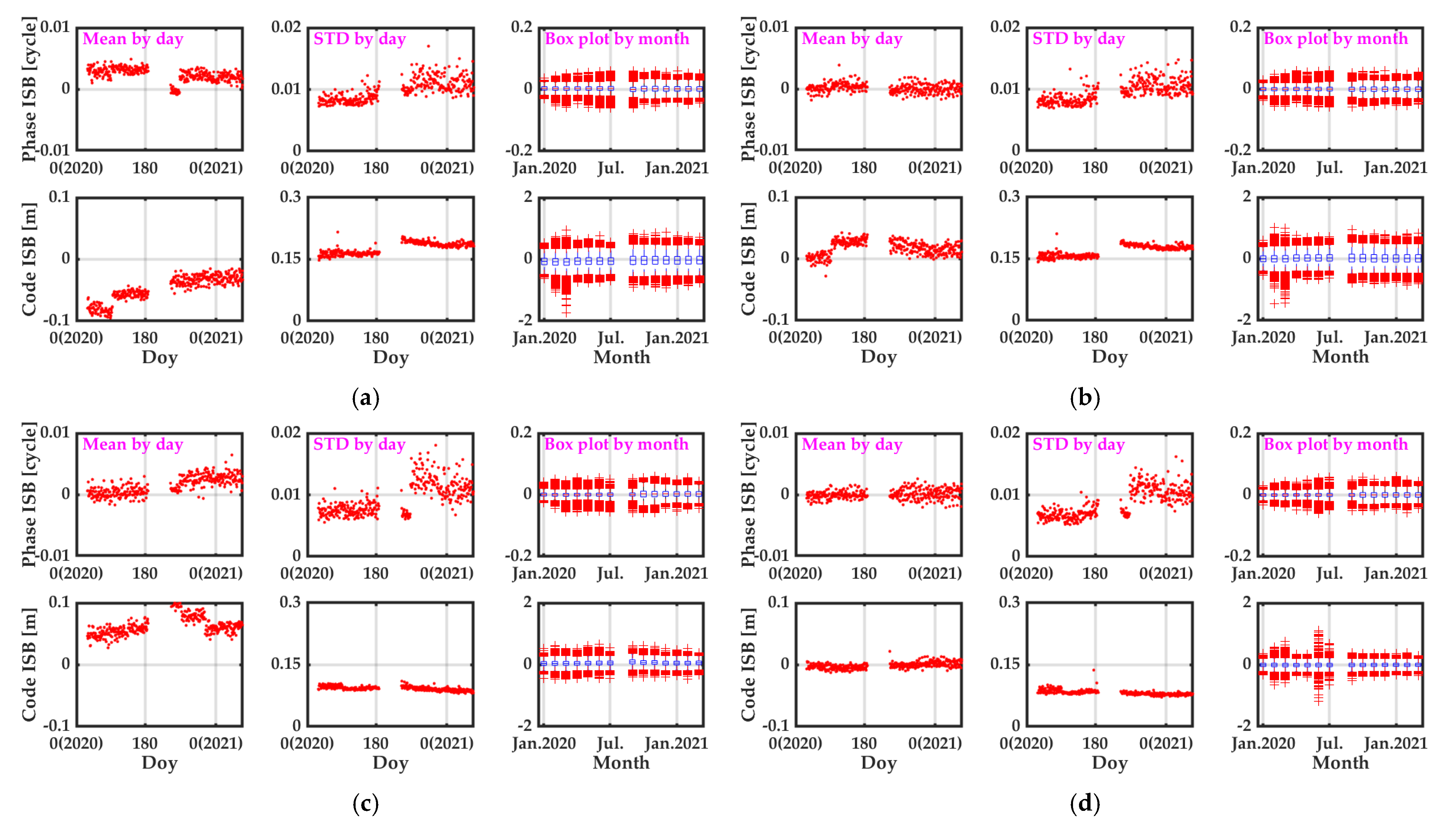
3.3.2. Long-Term ISB

Having assessed the short-term stability of ISB, it was reasonable to regard the ISB between identical types of receivers as a constant with continuous observations. However, we also needed to determine whether the ISB remains as stable in the long term as it does in the short term. In addition, by assessing the long-term ISB, we further analyzed its distribution characteristics through its PDF and QQ of normal distribution.

The time-series, PDF, and QQ plot of both phase and code ISBs between BDS-3 and GPS/Galileo are shown in Figure 5 for B1C/L1/E1 and B2a/L5/E5a. The results from DOY 29 to 70, 2021 were considered to validate the stability of ISBs. The relationship between the distribution characteristics of ISBs and the normal distribution was discussed. The figure shows that the level of the long-term ISB stability remains as low as it does in the short term. In addition, per both the PDF and QQ plot, the distribution of ISB fits a normal distribution well. This means that we can consider the ISB between identical types of receivers as random noise. Despite the higher noise appearing in the code ISB in B1C/L1/E1, the noise level of ISB between B1C/L1/E1 and B2a/L5/E5a is within the accuracy of the code observations. For the phase ISB, all the noise of phase ISB is about 0.01 cycles, which is also within the accuracy of phase observations. All the results prove that the ISBs between identical types of receivers have similar characteristics: zero-mean random noise and the noise level is similar to observation noise. Thus, the ISBs can be regarded as a constant even in the long term.

The noise level of ISB varies in different periods, which is mainly influenced by the number of visible satellites, the elevation of the satellites in the pivot system, the environment, the receiver firmware, etc. Thus, an analysis on the statistics of ISBs within one day or one month was is necessary to validate the long-term ISB stability. Figure 6 shows the mean value by day, STD by day, and box plot by month of both phase and code ISBs with the overlapping frequency between BDS-3/GPS/Galileo from DOY 29 to 70, 2021. The mean value of phase ISB is close to zero during the period, while that of code ISB varies within 10 cm. In addition, the STDs of all the phase ISB are around 0.01 cycles for various days, whereas that of code ISB is within 0.2 m for B1C/L1/E1 and 0.12 m for B2a/L5/E5a. The box plots reflect the discrete values of ISBs in the statistics. In the box plots, the quartile of each month remains at a level lower than 0.01 cycles for phase ISB and 0.2 m for code ISB. Even the outliers remain lower than 0.06 cycles for phase ISB and 1.6 m for code ISB. All the results indicate that the ISBs between identical types of receivers are quite stable even in the long term, and they fit a normal distribution well. Thus, if an overlapping frequency inter-system DD is performed, we can ignore the influence of ISBs when identical types of receivers are applied. Then, the TCM RTK can be obtained to avoid the waste of pivot satellites. Importantly, we found the phase ISBs maintained zero-mean characteristics for all the frequency pairs over the entire period, because the phase ISBs may seriously impact ambiguity resolution in TCM. Once we ignore the influence of phase ISBs, they may destroy the integer nature of the DD ambiguity so that ambiguity resolution becomes difficult.

3.4. Performance of RTK Positioning

In this last part, we discuss the stability of the ISB between BDS-3/GPS/Galileo in the short and long term. The results show that we can ignore the impact of ISB when the overlapping frequency inter-system DD is applied between identical-type receivers. In this part, we first compare the performance of single-system (SS), dual-frequency (DF) RTK with that of triple-system (TS) DF RTK. Then, the positioning performance of TCM RTK is assessed with respect to LCM RTK. Finally, the positioning accuracy and success rate of the ambiguity resolution under different cutoff elevation angles are analyzed. All RTK positioning is based on instantaneous mode and the SR is computed through dividing the epochs correctly fixed by the total epochs. In RTK processing, we used the Saastamoinen model and Klobuchar model to correct the tropospheric and ionospheric delay, respectively. The broadcast ephemeris is used to compute the position of satellites. The noise of code and phase observations are set to 0.3 m and 0.003 m, respectively. The ambiguity resolution was validated by comparison with the corresponding continuous RTK. The pivot satellites were chosen based on the elevation angle of the satellites. The satellite with highest elevation angle was selected as the pivot satellite for a single constellation (LCM) or mixed constellation (TCM). All the ambiguity resolutions are based on instantaneous RTK and the empirical SR is reported.

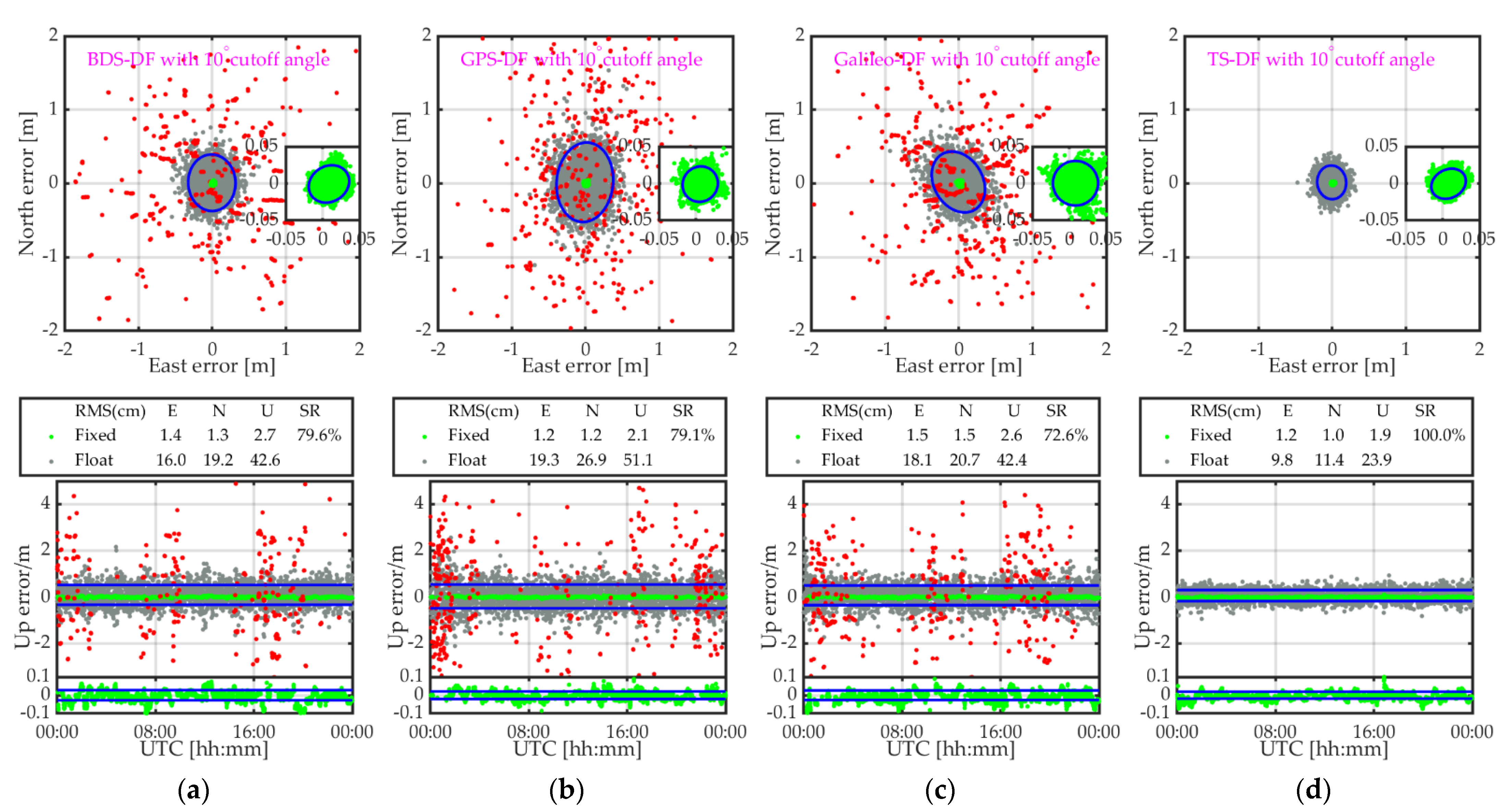
3.4.1. Single System vs. Multi System

Figure 7 displays the positioning errors of SS-DF and TS-DF RTK of the GODE-USN7 baseline on DOY 120, 2021 with a cutoff elevation angle of 10°. To evaluate the SR and positioning accuracy of different RTK modes, the statistics of the positioning errors are shown at the top of the time series of vertical errors through the RMS in centimeters. For the SS RTK, despite having the most satellites in GPS, only 12 BLOCK IIF and 4 III-A satellites can transmit the L5 signal. Thus, the SR and accuracy of the float solution of GPS-DF RTK are slightly lower than those of BDS-DF. However, demonstrated by the accuracy of the correctly fixed solution, the GPS performs the best in SS-DF RTK. Galileo has a similar positioning accuracy to BDS-3 but a lower SR. With the TS applied, the SR and the positioning accuracy improve considerably. The SR of TS-DF RTK is to 100%, whereas the SRs of SS-DF remain lower than 80%. Compared with SS-DF, the positioning accuracy of TS-DF improves over 40% in the float solution and 9% in the correctly fixed solution. The results of RTK positioning in different modes indicate that when more systems are applied, a sufficient number of satellites ensures correctly fixed ambiguity resolution, and the better distribution of satellites increases the positioning accuracy of both the fixed and float solutions.

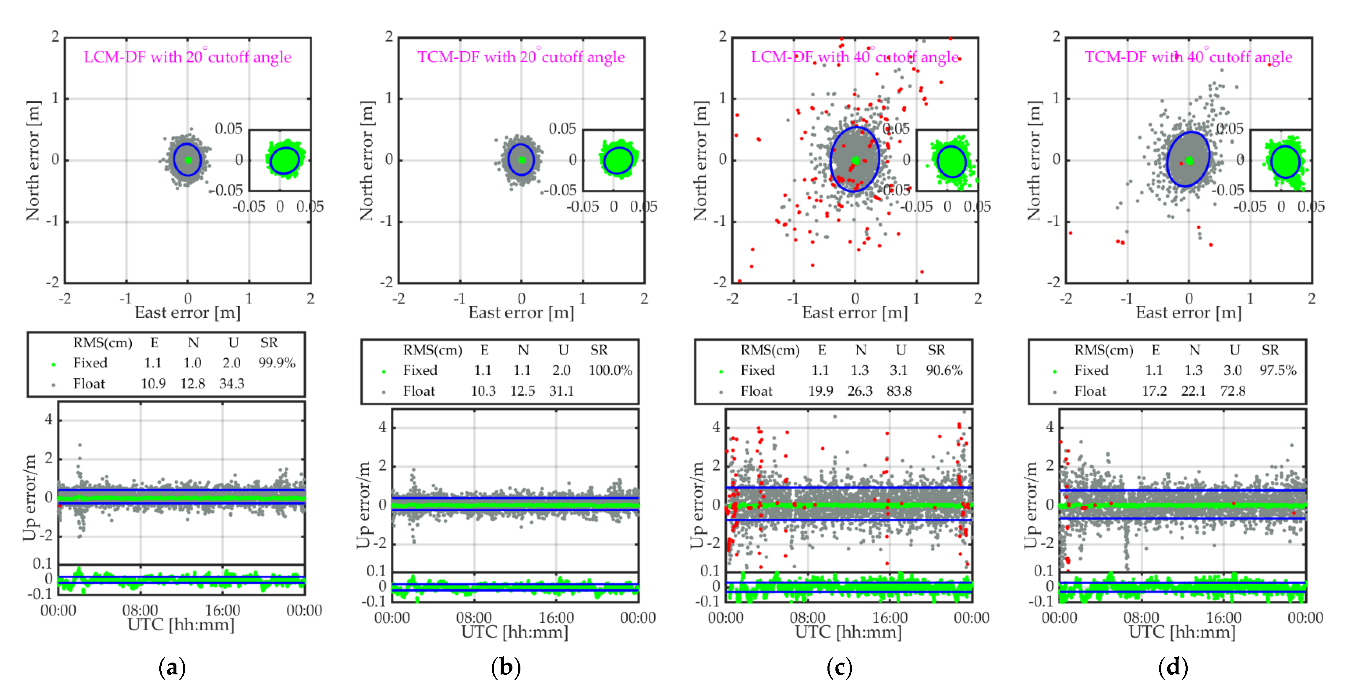
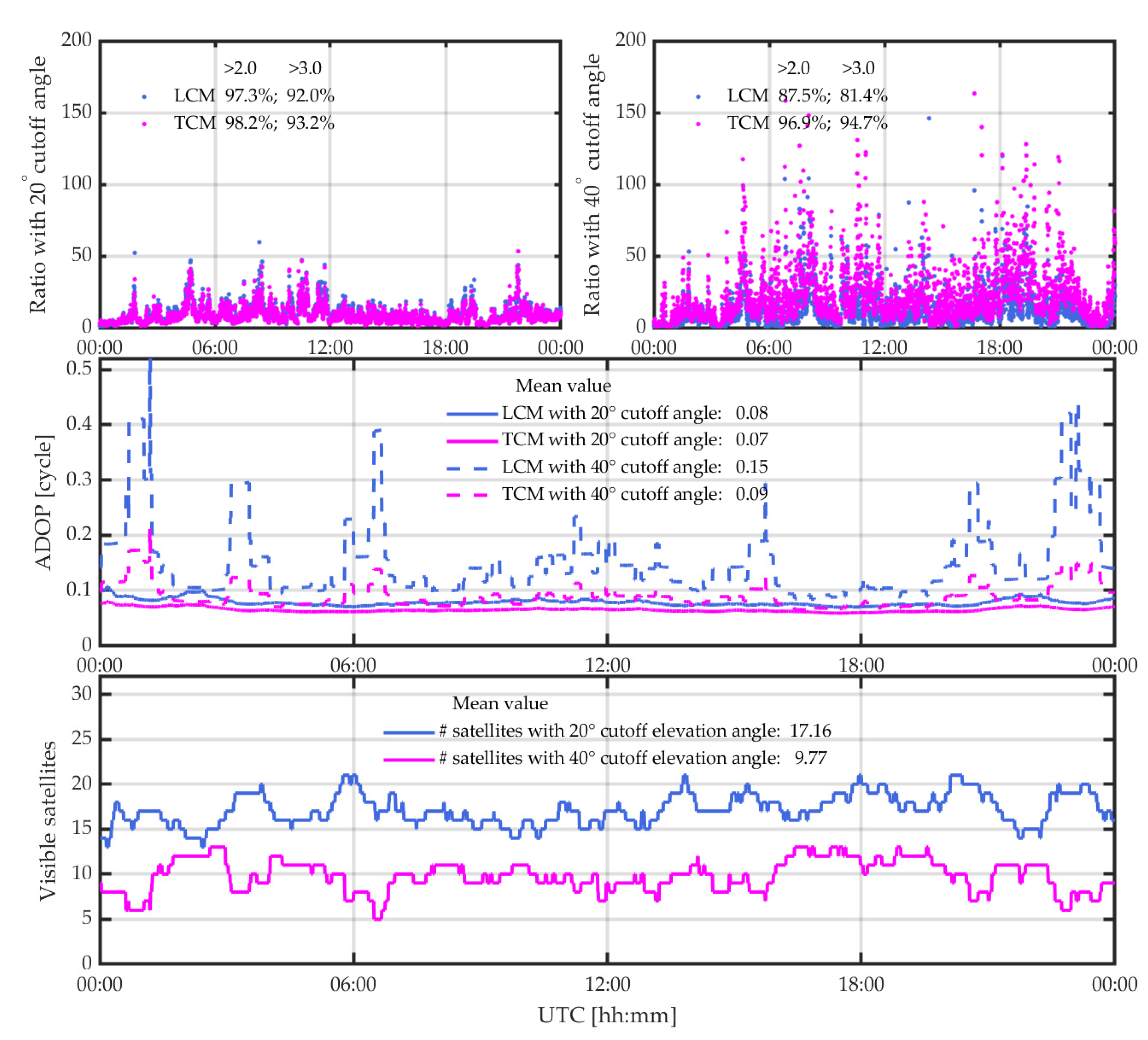
3.4.2. LCM RTK vs. TCM RTK

The ambiguity dilution of precision (ADOP) is an easy-to-compute scale diagnostic that can reflect the precision of ambiguity resolution, which is defined as [36]:

$$ADOP={\left|Q_{\widehat{a}}\right|}^{\frac{1}{2n}}$$

(10)

where $Q_{\widehat{a}}$ is the variance-covariance matrix of ambiguity $\widehat{a}$ with a dimension of $n$. The ADOP unit (cycles) is the same as that of ambiguity. A lower ADOP corresponds to a higher probability of correctly fixed solutions. Odijk [37] described more characteristics of ADOP and provided one conclusion: an ADOP smaller than 0.12 cycles may have a success rate above 99.9%. In this part, the ADOP is used as one of the criteria used to evaluate the ambiguity resolution to assess the performance of TCM RTK with respect to LCM RTK.

In Section 3.4.1, we analyzed the performance of SS and TS LCM RTK positioning with a cutoff elevation angle of 10°. Considering the larger visible satellites (about 22.89, as shown in Figure 1) with an elevation angle over 10°, in this section, we limit the cutoff elevation angle to 20 and 40° to compare the positioning performance of LCM and TCM with higher cutoff elevation angles. Figure 8 shows the positioning errors of TS LCM and TCM RTK of the baseline GODE-USN7 on DOY 120, 2021 with cutoff elevation angles of 20 and 40°. Due to the relatively sufficient number of satellites with an elevation over 20°, the LCM and TCM RTK can achieve an SR near 100%. The positioning accuracy of the float solution of TCM is higher than that of LCM, whereas the positioning accuracies of the fixed solutions remains similar. With the cutoff elevation angle raised to 40°, not only the positioning accuracy, but the SRs of both LCM and TCM decrease obviously. Under such a high cutoff elevation angle, both positioning accuracy and SR in TCM significantly improve compared with LCM. When TS observations were applied, three pivot satellites are necessary in LCM, whereas only one pivot satellite is enough in TCM. Therefore, if only one satellite exists in a system, this satellite will be abandoned in LCM RTK. In TCM RTK, this single satellite can also work in positioning through the inter-system DD. This means TCM RTK helps with using more satellites and a significant improvement in positioning performance occurs when the satellites are insufficient. From the results of the experiments, with a cutoff elevation angle of 40°, 7.7 and 13.4% improvements in the SR and accuracy of the float solution with TCM RTK were achieved, respectively, compared with LCM RTK.

Figure 9 shows the ratio, ADOP, and number of visible satellites of LCM and TCM RTK with cutoff elevation angles of 20 and 40° for baseline GODE-UNS7. From the plots and legends, it can be found that the ratio of TCM is apparently higher than that of LCM. The percentage of the ratio over 3.0 remains at a high level, about 95%, even with a high cutoff elevation angle of 40°, whereas that of LCM is lower than 82%. With the higher cutoff elevation angle, the value of the ratio increases more in TCM than in LCM (10.7% increase in ratio over 2.0, and 16.3% increase in ratio over 3.0). For the ADOP, the TCM RTK corresponds to a lower value of ADOP over the entire observation period, which means the TCM has a higher precision of ambiguity than LCM. The same as for the ratio performance, with the higher cutoff elevation angle of 40°, more improvement in ADOP occurs in TCM RTK. With such a high cutoff elevation angle, the mean value of ADOP of LCM RTK reaches up to 0.15 cycles, whereas that of TCM RTK remains lower than 0.1 cycles. The average numbers of visible satellites with cutoff elevation angles of 20 and 40° are 17.16 and 9.77, respectively. The series of ratio and ADOP reflect the advantage of TCM in ambiguity resolution. With the same satellites, better performance and more reliable results can be guaranteed with TCM RTK.

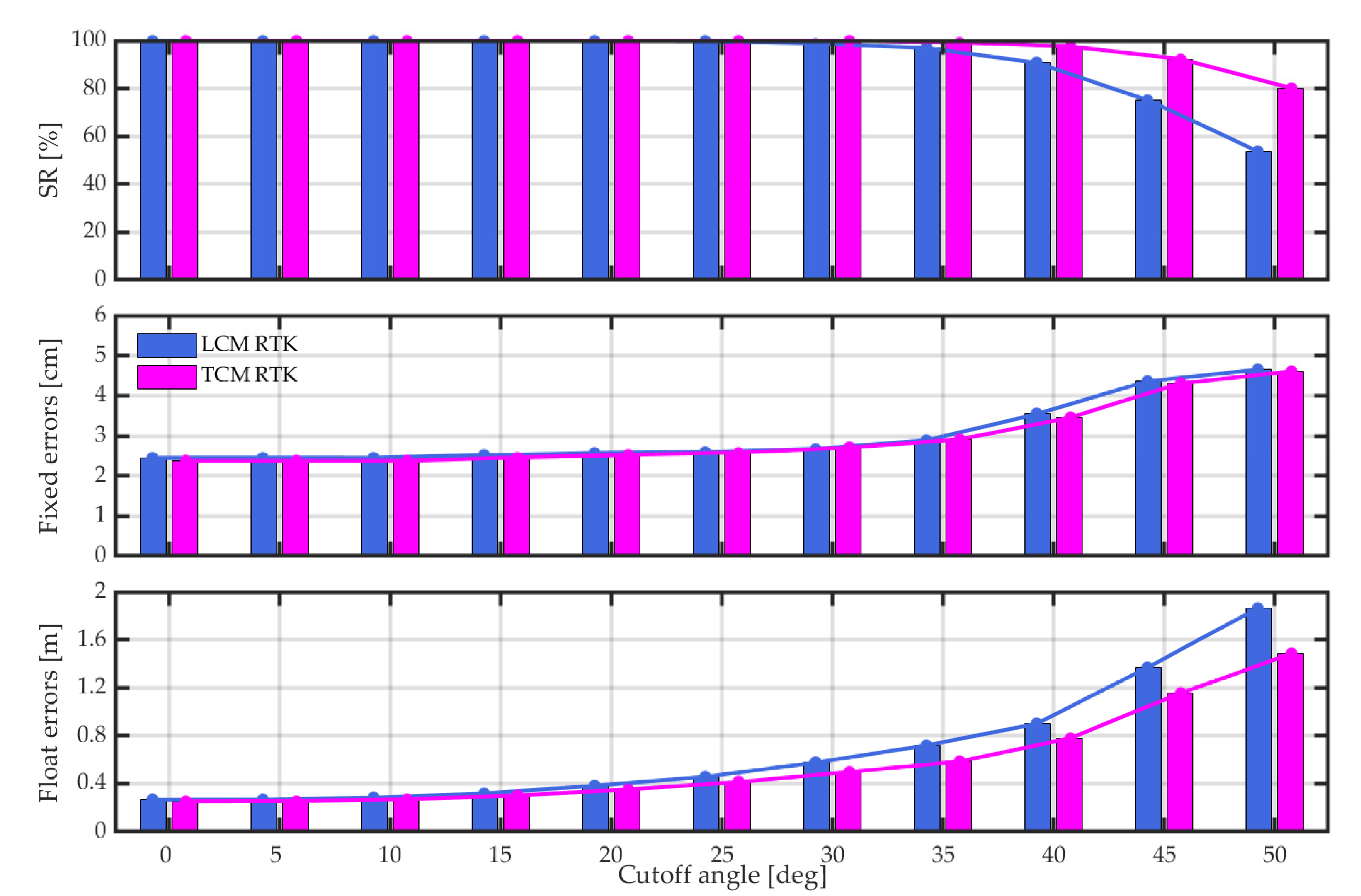
3.4.3. SR and Accuracy under Different Cutoff Elevation Angles

To assess the difference in the positioning performance of LCM and TCM RTK, a series of cutoff elevation angles was set from 0 to 50° with an interval of 5° to validate the improvement provided by TCM RTK with respect to LCM RTK, as shown in Figure 10. The corresponding statistics (SR and STD) of the correctly fixed solution and float solution are listed in

Table 5. The SR, accuracy of both the correctly fixed and float solutions of LCM and TCM RTK, and the corresponding improvement in TCM RTK with respect to LCM RTK.

Elevation (°)	SR (%)			Correctly Fixed Solution (cm)			Float Solution (m)
	LCM	TCM	Imp. 1	LCM	TCM	Imp.	LCM	TCM	Imp.
0	100	100	-	2.45	2.37	3.27%	0.27	0.25	7.41%
5	100	100	-	2.45	2.37	3.27%	0.27	0.26	3.70%
10	100	100	-	2.45	2.37	3.27%	0.28	0.27	3.57%
15	100	100	-	2.52	2.46	2.38%	0.32	0.30	6.25%
20	99.89	100	0.11%	2.57	2.52	1.95%	0.38	0.35	7.89%
25	99.72	100	0.28%	2.60	2.58	7.69%	0.46	0.41	10.87%
30	98.71	100	1.31%	2.68	2.70	-0.77%	0.58	0.50	13.79%
35	96.80	99.13	2.41%	2.89	2.91	-0.69%	0.72	0.59	18.06%
40	90.59	97.47	7.60%	3.54	3.45	2.5%	0.90	0.78	13.33%
45	75.20	92.16	22.55%	4.36	4.31	11.47%	1.37	1.15	16.06%
50	53.62	80.20	49.57%	4.66	4.60	12.87%	1.86	1.49	19.89%

¹ Imp., the improvements in the SR and positioning accuracy of TCM RTK with respect to LCM RTK.

. The SR and STD of the three-dimensional errors of both the correctly fixed solution and float solution of LCM and TCM RTK under different cutoff elevation angles are displayed as well. It can be observed that with increasing cutoff elevation angle, the SR and positioning accuracy obviously decrease. The significant increase in SR in TCM RTK with respect to LCM RTK when a high cutoff elevation angle is applied provides more application in RTK positioning. For example, an unusual cutoff elevation angle over 40° can be applied when the rover station is surrounded by buildings, suffering high-level multipath interference, etc. Though the correctly fixed solution retains centimeter-level precision, it varies from about 2–3 cm to about 4–5 cm as the cutoff elevation angle increases. Little improvement was found in the accuracy of the correctly fixed solution of TCM RTK with respect to LCM RTK. For the float solution, more obvious improvement in TCM RTK occurs with increasing cutoff elevation angle. An improvement in the float solution of about 20% can be achieved by TCM RTK with respect to LCM RTK with a high cutoff elevation angle of 50°. The results demonstrate that the TCM RTK can achieve higher positioning accuracy and higher SR in ambiguity resolution due to the extra redundant observations from the unnecessary pivot satellites. With increasing cutoff elevation angle, the satellites saved through choosing the common pivot satellite among the mixed constellation play an increasingly important role in the improvement in positioning performance.

4. Discussion

In this work, the models of LCM and TCM RTK together with the ISB estimation were first derived in Section 2. Then, with the observations collected from the IGS, we assessed the performance of signal quality in BDS-3/GPS/Galileo in terms of pseudo range multipath and TF phase combination by computing the statistics with an elevation interval of 2°. The results showed the better performance of B2a/L5/E5a in pseudo range multipath than B1C/L1/E1. Specifically, the RMS of pseudo range multipath of B2a/L5/E5a is 0.1–0.2 m lower than that B1C/L1/E1 for all the considered elevations. As for the TF phase combination, with the three different frequencies used, we compared its RMS in different GNSSs. With the IFCB corrected, the largest RMS of TF phase combination appears in Galileo for all the elevations. The RMS of BDS-3 remains at a similar level to GPS when the elevation is higher than 40°. However, the lowest RMS appears in BDS-3 when the elevation is lower than 40°.

Then, the short- and long-term stability of ISBs was evaluated with identical types of receivers. For the short-term ISB, both phase and code ISBs had a low STD within the precision of observations and a zero mean. Thus, it is reasonable to regard the ISB between identical types of receivers as a constant with continuous observations. Further research was conducted on the stability of long-term ISB. The PDF and the QQ plot demonstrated the stability of the long-term ISBs of both phase and code observation. The ISBs fit with the zero-mean normal distribution so well that we can regard the ISBs as random noise and ignore them in inter-system DD observations. The mean value and STD within the day and the boxplot within the month were also analyzed to validate the long-term stability of ISBs. The results showed the mean value of phase ISB is close to zero during the period whereas that of code ISB varies within 10 cm. In addition, the STDs of all the phase ISBs is around 0.01 cycles on various days, whereas that of code ISB is within 0.2 m between B1C/L1/E1 and 0.12 m between B2a/L5/E5a. In the box plots, even the outliers remain lower than 0.06 cycles for phase ISB and 1.6 m for code ISB. The statistics of the ISBs demonstrate that the ISBs can be regarded as a fixed bias that can be calibrated in advance and corrected in the inter-system DD observations. In addition, the zero-mean characteristics of ISBs between identical types of receivers mean the ISBs can be corrected by ignoring them directly.

Finally, we assessed the performance of RTK positioning with different models. The comparison of SS RTK with TS RTK demonstrated that when more satellites are applied, a better configuration of the mixed constellation is obtained, so the positioning of both the float and fixed solutions and the SR of the ambiguity resolution are much higher in TS RTK. With TS applied, 100% SR can be achieved, but the SR of SS RTK remains under 80%. However, with increasing cutoff elevation angle, the position accuracy and the SR decrease obviously when the conventional RTK (LCM RTK) is applied. A 90.6% SR can be achieved in LCM RTK with a cutoff elevation angle of 40°. However, with the ISB ignored in the inter-system difference observations from identical-type receivers, TCM RTK can achieve a higher SR of 96.5% and a higher positioning accuracy than LCM RTK. The significant increase in SR demonstrates the advantages of TCM RTK at a high cutoff elevation angle: with fewer pivot satellites chosen, more measurements can be used to achieve higher performance, and one satellite is enough in a mixed constellation to enhance the model. Assessing the performance of LCM and TCM RTK under different cutoff elevation angles in 5° intervals from 0 to 50°, we found that the improvement in performance with TCM RTK becomes even more obvious with respect to LCM RTK as the cutoff elevation angle increases. In addition, the improvement provided by TCM RTK validated that it is correct to ignore the ISBs between identical types of receivers and the ISB-corrected model TCM RTK logically improves RTK positioning.

5. Conclusions

From the summary of the main aspects of this study, we found that the differential ISBs of both code and phase observations remain stable even in the long term. Thus, the ISBs can be regarded as random noise within the accuracy of code and phase observations. The zero-mean characteristics of the ISB of identical-type receivers enable the ISBs to be ignored in inter-system DD observations, so the TCM RTK can be achieved with overlapping frequency observations applied. The TCM RTK need only one pivot satellite in the mixed constellation and more redundancy can be obtained in the function model. For instance, in the overlapping-frequency TS-DF RTK, three pivot satellites are necessary in the LCM RTK, whereas only one pivot satellite is required in the TCM RTK. Thus, four (2 × 2) more redundant observations can be obtained in the TCM than in LCM, resulting in a stronger functional model and improved performance in multi-GNSS positioning. The improvement in SR in TCM RTK is over 49% with an increasing cutoff elevation angle with respect to LCM RTK, with an obvious improvement in the positioning accuracy also found.

References

1. Montenbruck, O.; Steigenberger, P.; Khachikyan, R.; Weber, G.; Langley, R.; Mervart, L.; Hugentobler, U. IGS-MGEX: Preparing the Ground for Multi-Constellation. GNSS Sci. 2014, 9, 42–49. [Google Scholar]
2. CSNO. Development of the BeiDou Navigation Satellite System (Version 4.0); China Satellite Navigation Office Technical Report; CSNO: Washington, DC, USA, 2019. [Google Scholar]
3. Hou, P.; Zhang, B.; Yuan, Y. Combined GPS+BDS instantaneous single- and dual-frequency RTK positioning: Stochastic modelling and performance assessment. J. Spat. Sci. 2019, 66, 3–26. [Google Scholar] [CrossRef]
4. Su, K.; Jin, S. Triple-frequency carrier phase precise time and frequency transfer models for BDS-3. GPS Solut. 2019, 23, 86. [Google Scholar] [CrossRef]
5. CSNO. BeiDou Navigation Satellite System Open Service Performance Stand (Version 3.0); China Satellite Navigation Office Technical Report; CSNO: Washington, DC, USA, 2021. [Google Scholar]
6. Zhang, Y.; Kubo, N.; Chen, J.; Wang, J.; Wang, H. Initial Positioning Assessment of BDS New Satellites and New Signals. Remote Sens. 2019, 11, 1320. [Google Scholar] [CrossRef] [Green Version]
7. Yang, Y.; Gao, W.; Guo, S.; Mao, Y.; Yang, Y. Introduction to BeiDou-3 navigation satellite system. Navigation 2019, 66, 7–18. [Google Scholar] [CrossRef] [Green Version]
8. Zhang, X.; Wu, M.; Liu, W.; Li, X.; Yu, S.; Lu, C.; Wickert, J. Initial assessment of the COMPASS/BeiDou-3: New-generation navigation signals. J. Geod. 2017, 91, 1225–1240. [Google Scholar] [CrossRef]
9. NOAA. Space Segment. Available online: https://www.gps.gov/systems/gps/space/ (accessed on 5 August 2021).
10. Centre, E.G.S. (European GNSS Service). Constellation Information. Available online: https://www.gsc-europa.eu/system-service-status/constellation-information (accessed on 5 August 2021).
11. Kubo, N. Advantage of velocity measurements on instantaneous RTK positioning. GPS Solut. 2009, 13, 271–280. [Google Scholar] [CrossRef] [Green Version]
12. Angelo, F.N.; Gianpaolo, C.; Carmine, G.; Antonino, M.; Annamaria, V. A Test on the Potential of a Low Cost Unmanned Aerial Vehicle RTK/PPK Solution for Precision Positioning. Sensors 2021, 21, 3882. [Google Scholar]
13. Keshavarzi, H.; Lee, C.; Johnson, M.; Abbott, D.; Ni, W.; Campbell, D.L. Validation of Real-Time Kinematic (RTK) Devices on Sheep to Detect Grazing Movement Leaders and Social Networks in Merino Ewes. Sensors 2021, 21, 924. [Google Scholar] [CrossRef] [PubMed]
14. Gao, W.; Gao, C.; Pan, S. A method of GPS/BDS/GLONASS combined RTK positioning for middle-long baseline with partial ambiguity resolution. Surv. Rev. 2016, 49, 212–220. [Google Scholar] [CrossRef]
15. Hofmann-Wellenhof, B.; Lichtenegger, H.; Wasle, E. GNSS—Global Navigation Satellite Systems: GPS, GLONASS, Galileo, and More; Springer Science & Business Media: New York, NY, USA, 2007. [Google Scholar]
16. Odolinski, R.; Teunissen, P.J.G.; Odijk, D. First combined COMPASS/BeiDou-2 and GPS positioning results in Australia. Part II: Single- and multiple-frequency single-baseline RTK positioning. J. Spat. Sci. 2014, 59, 25–46. [Google Scholar] [CrossRef]
17. Edwards, S.J.; Clarke, P.J.; Penna, N.T.; Goebell, S. An Examination of Network RTK GPS Services in Great Britain. Surv. Rev. 2013, 42, 107–121. [Google Scholar] [CrossRef] [Green Version]
18. Lemmon, T.R.; Gerdan, G.P. The Influence of the Number of Satellites on the Accuracy of RTK GPS Positions. Aust. Surv. 2012, 44, 64–70. [Google Scholar] [CrossRef]
19. Pirti, A. Performance Analysis of the Real Time Kinematic GPS (RTK GPS) Technique in a Highway Project (Stake-Out). Surv. Rev. 2013, 39, 43–53. [Google Scholar] [CrossRef]
20. Odolinski, R.; Teunissen, P.J.G. Single-frequency, dual-GNSS versus dual-frequency, single-GNSS: A low-cost and high-grade receivers GPS-BDS RTK analysis. J. Geod. 2016, 90, 1255–1278. [Google Scholar] [CrossRef]
21. Odolinski, R.; Teunissen, P.J.G. Low-cost, high-precision, single-frequency GPS–BDS RTK positioning. GPS Solut. 2017, 21, 1315–1330. [Google Scholar] [CrossRef]
22. Teunissen, P.J.G.; Odolinski, R.; Odijk, D. Instantaneous BeiDou+GPS RTK positioning with high cut-off elevation angles. J. Geod. 2013, 88, 335–350. [Google Scholar] [CrossRef]
23. Li, J.; Yang, Y.; Xu, J.; He, H.; Guo, H.; Wang, A. Performance Analysis of Single-Epoch Dual-Frequency RTK by BeiDou Navigation Satellite System. In China Satellite Navigation Conference (CSNC) 2013 Proceedings; Lecture Notes in Electrical Engineering; Springer: Berlin/Heidelberg, Germany, 2013; Volume 245, pp. 133–143. [Google Scholar] [CrossRef]
24. Odijk, D.; Teunissen, P.J.G. Characterization of between-receiver GPS-Galileo inter-system biases and their effect on mixed ambiguity resolution. GPS Solut. 2012, 17, 521–533. [Google Scholar] [CrossRef]
25. Odijk, D.; Teunissen, P.J.G.; Huisman, L. First results of mixed GPS+GIOVE single-frequency RTK in Australia. J. Spat. Sci. 2012, 57, 3–18. [Google Scholar] [CrossRef]
26. Odijk, D.; Nadarajah, N.; Zaminpardaz, S.; Teunissen, P.J.G. GPS, Galileo, QZSS and IRNSS differential ISBs: Estimation and application. GPS Solut. 2016, 21, 439–450. [Google Scholar] [CrossRef]
27. Mi, X.; Zhang, B.; Yuan, Y.; Luo, X. Characteristics of GPS, BDS2, BDS3 and Galileo inter-system biases and their influence on RTK positioning. Meas. Sci. Technol. 2020, 31, 015009. [Google Scholar] [CrossRef]
28. Wu, L.; Wang, Z. Differential Inter-System Biases Estimation and Initial Assessment of Instantaneous Tightly Combined RTK with BDS-3, GPS, and Galileo. Remote Sens. 2019, 11, 1430. [Google Scholar] [CrossRef] [Green Version]
29. Zhang, B.; Teunissen, P.J.G. Characterization of multi-GNSS between-receiver differential code biases using zero and short baselines. Sci. Bull. 2015, 60, 1840–1849. [Google Scholar] [CrossRef] [Green Version]
30. Zhang, B.; Teunissen, P.J.G.; Yuan, Y.; Zhang, X.; Li, M. A modified carrier-to-code leveling method for retrieving ionospheric observables and detecting short-term temporal variability of receiver differential code biases. J. Geod. 2018, 93, 19–28. [Google Scholar] [CrossRef] [Green Version]
31. Teunissen, P.J.G. The least-squares ambiguity decorrelation adjustment: A method for fast GPS integer ambiguity estimation. J. Geod. 1995, 70, 1–2. [Google Scholar] [CrossRef]
32. Wang, K.; Teunissen, P.J.G.; El-Mowafy, A. The ADOP and PDOP: Two Complementary Diagnostics for GNSS Positioning. J. Surv. Eng. 2020, 146, 04020008. [Google Scholar] [CrossRef] [Green Version]
33. Estey, L.H.; Meertens, C.M. TEQC: The Multi-Purpose Toolkit for GPS/GLONASS Data. J. GPS Solut. 1999, 3, 42–49. [Google Scholar] [CrossRef]
34. Zhang, Z.; Li, B.; Nie, L.; Wei, C.; Jia, S.; Jiang, S. Initial assessment of BeiDou-3 global navigation satellite system: Signal quality, RTK and PPP. GPS Solut. 2019, 23, 1–12. [Google Scholar] [CrossRef]
35. Miao, W.; Li, B.; Zhang, Z.; Zhang, X. Combined BeiDou-2 and BeiDou-3 instantaneous RTK positioning: Stochastic modeling and positioning performance assessment. J. Spat. Sci. 2019, 65, 7–24. [Google Scholar] [CrossRef]
36. Teunissen, P.J.G. A canonical theory for short GPS baselines. Part II: The ambiguity precision and correlation. J. Geod. 1997, 71, 389–401. [Google Scholar] [CrossRef]
37. Odijk, D.; Teunissen, P.J.G. ADOP in closed form for a hierarchy of multi-frequency single-baseline GNSS models. J. Geod. 2008, 82, 473–492. [Google Scholar] [CrossRef] [Green Version]
Figure 1. (a) Sky plots of BDS-3 (in blue), GPS (in green), and Galileo (in magenta) on day of year (DOY) 120, 2021 at GODN. (b) The number of visible satellites of the different global navigation satellite systems (GNSSs) and all the GNSSs (in red). (c) The position dilution of precision (PDOP) time-series of different GNSSs and all the GNSSs. In addition, the average number of visible satellites within the day is shown in the legend and all the statistics were computed with a cutoff elevation angle of 10°.
Remotesensing 13 03507 g001
Figure 2. Root mean square (RMS) of multipath (MP) vs. elevation angle of all the observed signals in BDS-3, GPS, and Galileo. The RMS of MP of every 2° of elevation of all the signals were computed with the whole constellation that can be tracked.
Remotesensing 13 03507 g002
Figure 3. (a) Time series of the TF phase combination extracted by the observations from C19, G01, and E01. (b) The RMS of TF phase MP vs. elevation angle of BDS-3, GPS, and Galileo computed with the whole constellation that can be tracked of every 2° of elevation with inter-frequency clock bias (IFCB) corrected by the baseline GODN-GODS.
Remotesensing 13 03507 g003
Figure 4. Inter-system bias (ISB) time series of both phase and code observations between BDS-3 and GPS/Galileo for the overlapping frequencies B1C/L1/E1 and B2a/L5/E5a. From the left to the right, B1C/L1, B2a/L5, B1C/E1, and B2a/E5a observations on DOY 120, 2021 were applied to assess the ISBs. The text in magenta describes the statistics of the ISBs.
Remotesensing 13 03507 g004
Figure 5. Time-series, probability density function (PDF) and quantile against the quantile (QQ) plot of both phase and code ISBs between B1C/L1 (a), B1C/E1 (b), B2a/L5 (c), and B2a/E5a (d) with the observations from DOY 29 to 70, 2021 between the baseline GODN-GODS with identical types of receivers. The magenta line in the PDF of ISB denotes the empirical normal PDF. The x-axis of the QQ plot denotes the quantile of the standard normal distribution, while the y-axis denotes the quantile of our sample distribution as shown in the time series. The dotted line in the QQ plot denotes the empirical normal distribution of the sample against the standard normal distribution, while the scatters denote the real sample distribution.
Remotesensing 13 03507 g005
Figure 6. Means for one day, STD for one day, and box plot for one month of both phase and code ISBs between B1C/L1 (a), B1C/E1 (b), B2a/L5 (c), and B2a/E5a (d) with the observations from DOY 29 to 70, 2021 between the baseline GODN-GODS of identical-type receivers. The mean value and STD of ISBs were computed within one day, whereas the box plot was computed within one month. In the box plot, the blue line in the box denotes the median of the ISB for one month, while the top and bottom border of the box denote the quartiles of the ISB. The scatters in the box plot denote the outliers.
Remotesensing 13 03507 g006
Figure 7. Horizontal scatters (top) and vertical time series (bottom) of the positioning errors of BDS-3 (a), GPS (b), Galileo (c), and triple-system (TS) (d) dual-frequency (DF) RTK of baseline GODE-USN7 on DOY 120, 2021 with a cutoff elevation angle of 10°. On the right of the horizontal scatterplot and on the bottom of the vertical time series, the details of the fixed solutions are displayed with the 95% confidence interval. The float solutions, correct solutions, and incorrect solutions are indicated in grey, green, and red, respectively.
Remotesensing 13 03507 g007
Figure 8. Horizontal scatters (top) and vertical time series (bottom) of the positioning errors of loosely-combined model (LCM) (a,c) and tightly-combined model (TCM) (b,d) DF RTK of baseline GODE-USN7 on DOY 120, 2021 with a cutoff elevation angle of 20° (a,b) and 40° (c,d). On the right of the horizontal scatterplot and on the bottom of the vertical time series, details are provided about the fixed solutions with the 95% confidence interval. The float solutions, correct solutions, and incorrect solutions are indicated in grey, green, and red, respectively.
Remotesensing 13 03507 g008
Figure 9. Time series of ratio (top), ambiguity dilution of precision (ADOP) (middle), and number of visible satellites (bottom) of LCM and TCM RTK of baseline GODE-USN7 on DOY 120, 2021 with cutoff elevation angles of 20 and 40°. The blue and magenta indicate LCM and TCM, respectively.
Remotesensing 13 03507 g009
Figure 10. Success rate (SR) (top), three-dimensional errors of the correctly fixed solution and the float solution of LCM and TCM RTK positioning on DOY 120, 2021 for the baseline GODE-USN7 with different cutoff elevation angles ranging from 0 to 50°. The bars and lines denote the corresponding statistics.
Remotesensing 13 03507 g010