On the Assessment GPS-Based WRFDA for InSAR Atmospheric Correction: A Case Study in Pearl River Delta Region of China

Abstract

The accuracy and applications of synthetic aperture radar interferometry (InSAR) are severely suppressed by tropospheric error. Numerical Weather Models (NWMs) and GPS-derived tropospheric delays have been widely used to correct the tropospheric error considering their complete spatial coverage or high accuracy. However, few studies focus on the fusion of both NWMs and GPS for the tropospheric error correction. In this study, we used the Weather Research and Forecasting (WRF) to obtain NWMs with a higher spatial-temporal resolution of 3 km and 20 s from both ERAI (79 km and 6 h) and ERA5 (0.25° and 1 h). After that, we utilized the WRF Data Assimilation (WRFDA) system to assimilate the GPS ZTD into these enhanced NWMs and generate merged NWMs products. The tropospheric correction effectiveness from different NWMs products was evaluated in a case in the Pearl River Delta region of China. The results showed that all the NWMs products could correct the stratified component in the interferogram but could not mitigate the turbulence well, even after improving the spatial-temporal resolution. As for the trend component, the merged NWMs products showed obvious superiority over other products. From the statistics perspective, the stdev of the interferogram decreased further over 20% by the merged NWMs products than other products when using both ERAI and ERA5, indicating the significant effectiveness of GPS ZTD assimilation.

1. Introduction

Synthetic aperture radar interferometry (InSAR) has demonstrated a powerful measurement capability in a wide range of applications such as earthquake deformation [1], land subsidence [2], and volcanic activity monitoring [3,4]. However, similar to other spatial geodetic techniques, InSAR measurements are inevitably affected by the atmosphere, which is still an intractable limitation to high-accuracy applications and needs careful corrections [5,6,7].

There are mainly two methods to correct InSAR atmospheric delay [5], namely (1) by using the interferogram itself or (2) by using external atmospheric products (referred to EAP hereafter). The former method generally assumes atmospheric error as temporal random noise [8] or as an elevation-dependent component [9,10], which either needs a large set of interferograms to separate deformation rate and noise or relies on the assumption of correlations between the deformation and elevation. By contrast, the latter method, which is based on EAP, such as Global Positioning System (GPS) [11], Numerical Weather Models (NWMs) [12,13,14,15,16], and Moderate Resolution Imaging Spectroradiometer (MODIS) [17], can provide direct tropospheric delay correction and is more straightforward.

The temporal-spatial resolution and accuracy of EAP are vital for reliable InSAR atmospheric correction, which is, however, not satisfying for most EAP. For example, MODIS measurements are sensitive to the presence of clouds and need calibration [18]. NWMs product, such as ERA-Interim reanalysis (referred as ERAI hereafter) and operational analysis from the European Centre for Medium-range Weather Forecast (ECMWF), which has been widely used in many works of literature, can guarantee the complete spatial coverage for estimating atmospheric corrections [12,13,19,20]. Nevertheless, most current global NWMs are still insufficient in spatial resolution to capture the small-scale atmospheric water vapor turbulence affecting InSAR measurements [21]. The temporal-spatial resolution of NWMs can be further improved regionally by using tools like Weather Research and Forecasting (WRF) for InSAR atmospheric corrections [22]. However, Kinoshita et al. [23] stated that WRF only improves the spatial and temporal resolution but helps little to the accuracy of parameters that primarily relies on observations. Doin et al. [24] argued that combining mesoscale atmospheric simulations and data assimilation (DA) would be the most promising tool for correcting InSAR atmospheric delays. Yun et al. [25] assimilated meteorological data from the Global Telecommunications System (GTS) into Final Operational Global Analysis (FNL) with the WRF-3DVar data assimilation system and demonstrated the high potential and effectiveness of WRFDA in InSAR atmospheric correction.

The ground-based GPS has advantages of high accuracy, high temporal resolution, low cost, and continuous in all weather conditions for retrieving atmospheric delay or water vapor content [26]. Therefore, it is attractive to combine NWMs and GPS zenith total delay (ZTD) or water vapor content by data assimilation to generate merged NWMs. Yu et al. [13,27] applied an iterative tropospheric decomposition (ITD) method to combine NWMs with ground-based GPS and found that the combination products perform better than NWMs for InSAR corrections. However, this combination was conducted based on the interpolation of relative ZTDs but not data assimilation systems. Mateus et al. [28] carried out experiments in Lisbon city and found that WRF can reproduce the spatial atmospheric trend in the calibrated InSAR. There have also been some studies where InSAR and GPS ZTD were assimilated into NWMs by WRFDA to improve the weather forecast performance [29,30,31,32]. However, there are currently few studies assimilating GPS ZTD into NWMs for the InSAR correction.

Therefore, this paper will make a preliminary study to investigate the performance of correcting InSAR atmospheric delay by combining NWMs and GPS ZTD. Three kinds of NWMs, namely, the reanalysis, reanalysis-based WRF without GPS ZTD assimilation, and reanalysis-based WRF with GPS ZTD assimilation, will be compared. The paper is organized as follows: Section 2 introduces the InSAR atmospheric delay correcting method, the used InSAR and reanalysis data as well as the WRF and WRFDA configurations. Section 3 presents the corrected results and Section 4 makes some discussions, followed by the conclusions in Section 5.

2. Data and Methodology

In this section, the experiment setup and the related data will be introduced first, followed by the methods for generating different correcting products.

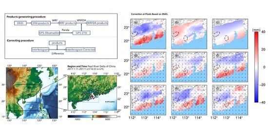
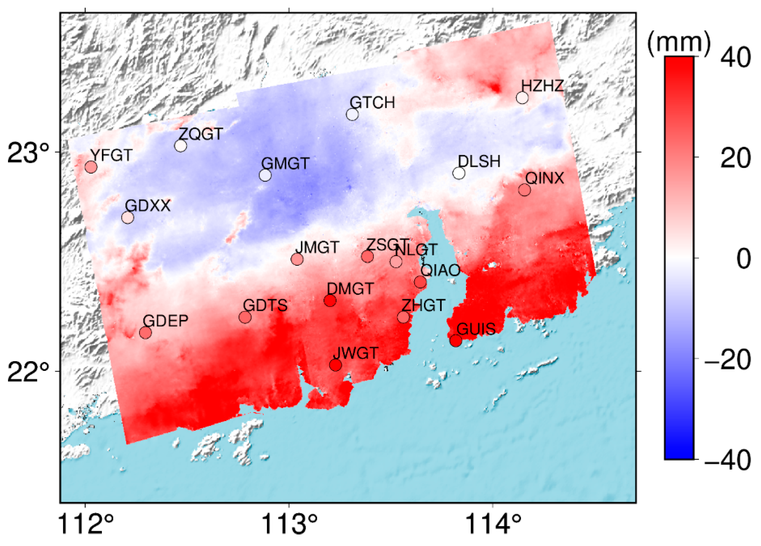
2.1. Study Area and InSAR Data Processing

A coastal area in the Pearl River Delta region, Guangdong province in the south of China, is selected as the study area, as shown in Figure 1, where atmospheric turbulences are usually stronger and harder to predict in NWMs than inland regions [33]. The SAR images of Sentinel-1A on 11/01/2017 and 23/01/2017 are selected to generate the interferogram. The acquisition time is 10:33 UTC, the perpendicular baseline is −17 m, and the flight direction is ascending. Terrain deformations are negligible considering the temporal baseline of only 12 days.

The interferogram was produced by using the ISCE software [34]. The USGS SRTM 30m digital elevation model (DEM) generated and corrected the topographic phase component. Precise orbits from the Copernicus POD (Precise Orbit Determination) Service were applied to eliminate the orbital error. The interferogram was unwrapped using the integrated correlation and unwrapping (ICU) package [35]. Additionally, the interferogram was multi-looked by $100\times 25$ looks in azimuth and range directions, respectively, and sampled to a final resolution of ~300 m.

2.2. Atmospheric Delay in InSAR

The phase observation of the interferogram, ${\varphi }_{obs}$, can be written as follows:

$${\varphi }_{obs}={\varphi }_{topo}+{\varphi }_{def}+{\varphi }_{orb}+{\varphi }_{atm}+{\varphi }_{\epsilon }$$

(1)

where ${\varphi }_{topo}$ is the phase caused by the topography, which can be reproduced by using the DEM and removed; ${\varphi }_{def}$ denotes the surface deformation component; ${\varphi }_{orb}$ is the component caused by the satellite orbital error, which is negligible when using the precise orbit ephemeris; ${\varphi }_{atm}$ represents the atmospheric delay where the ionospheric delay can be ignored for C-band InSAR such as the Sentinel-1 used in our study, and therefore only the tropospheric delay needs to be considered [36]; ${\varphi }_{\epsilon }$ denotes the un-modeled residual. The tropospheric delay can be divided into dry and wet delay following its physicochemical property or separated into the stratified component and the turbulence based on whether it is elevation-related or not [33]. The tropospheric delay in InSAR ($\delta L^{LOS}$) is the difference of delays at two SAR acquisition times and can be expressed as,

$$\delta L^{LOS}=∆L_r^{LOS}-∆L_s^{LOS}=\frac{ZT{D}_r}{\cos {\alpha }_r}-\frac{ZT{D}_s}{\cos {\alpha }_s}$$

(2)

where the subscript r and s represent reference and secondary interferogram. The tropospheric delay ($∆L^{LOS}$), which is also called slant total delay (STD), can be obtained by projecting ZTD onto the oblique path using the cosine function of incidence angle $\alpha$ in InSAR [37]. Therefore, the key to acquiring reliable atmospheric delay is to calculate ZTD for each pixel at the acquisition time accurately.

2.3. GPS Data Processing

There are 59 GPS stations in the study region, as shown in Figure 1b, where three stations experienced outages during the study period, resulting in 56 stations available in this work. The mean station spacing is about 35 km. The PANDA software [38] was used to process GPS observations in 30 s intervals with the precise point positioning (PPP) method in post-processing mode. Final satellite orbit and clock products from the International GNSS Service (IGS) (https://cddis.nasa.gov/archive/gnss/products/) (access on 8 June 2021) were used. The VMF3 model [39] was applied to estimate the a priori ZHD and the a priori ZWD and provide mapping functions. Residuals for the ZWD were estimated as piece-wise constants every 10 min with a power density of 15 mm ${\mathrm{h}}^{-1/2}$. The final GPS ZTDs were retrieved by summing the a priori ZHD, the a priori ZWD, and the estimated ZWD residuals. The tropospheric gradients, including the north–south and the east–west components, were estimated every two hours to account for the azimuthal asymmetry of the atmosphere. Receiver clocks were considered uncorrelated between successive epochs and were estimated every epoch. Station coordinates were estimated as daily constants. The cutoff elevation angle of satellites was set to 7°, and an elevation-dependent weighting strategy was applied [40]. The precision index of the estimated ZTDs output by the software was used for further designing the WRFDA assimilation weighting strategies.

2.4. Reanalysis and Data WRF Simulation

Two kinds of reanalysis data: ERAI and ERA5, both from the ECMWF, will be utilized in this paper. The ERAI dataset has a global coverage (except the poles) with a horizontal resolution of about 79 km and a temporal resolution of 6 h [41]. The ERA5 dataset is the latest reanalysis released by the ECMWF. Compared with its predecessor ERAI, ERA5 improves the temporal and spatial resolution to 1 h and 0.25°. In addition, ERA5 assimilates recent observations and newly reprocessed datasets, marking a potential improvement in overall quality and detail level [42]. The pressure-level reanalysis products, including the air temperature (T), air pressure (P), geopotential height (H), and specific humidity (Q), nearest the SAR acquisition time were used to calculate ZTD. In addition, the u/v components of wind in each pressure level, 10-m u/v wind components, skin temperature, surface pressure, and other surface parameters, were extracted to serve as the WRF initial and lateral boundary conditions.

The Weather Research and Forecasting Model is a mesoscale numerical weather prediction system designed for atmospheric research and operational forecasting applications [43]. The WRF can generate three-dimensional fields for meteorological parameters at a given time, taking NWMs as initial and boundary conditions and allow nests to achieve higher resolution. The WRF in version 4.2 was used in this work. Three two-way nested domains were set with a horizontal resolution of 27, 9, and 3 km, respectively, as shown in Figure 1. The air pressure at the top was set to be 10 hPa, and a total of 49 vertical levels were used in eta vertical coordinate, with the thickness of the top layer and lowest layer of 1000 and 50 m, respectively. The Goddard 4-ice microphysics scheme [44] was used for microphysics. The Kain–Fritsch scheme [45] was applied for the cumulus parameterization on domain d01 and d02, and domain d03 was regarded as convection-permitting [25]. The Dudhia scheme [46] was used for the shortwave radiation, and the Rapid Radiative Transfer Model (RRTM) [47] was used for the longwave radiation. The Yonsei University (YSU) [48] scheme was used for the planetary boundary layer. ERA5 and ERAI were used separately to provide the atmosphere and land surface initial and lateral boundary conditions. The cold start initialization was implemented and reanalysis data from 6:00 to 12:00 were used to cover the SAR acquisition time (10:33 UTC). Time steps were set as 180 s, 60 s, and 20 s for d01, d02, and d03, respectively.

The air temperature (T), air pressure (P), height (H), and specific humidity (Q) are needed to calculate ZTD where T, P, and H are WRF output variables, and Q can be converted from the water vapor mixing ratio ($QVAPOR$) by,

$$Q=QVAPOR/\left(1+QVAPOR\right)$$

(3)

The NCAR command language (NCL) [49] is used to extract parameters from WRF outputs and to make further interpolation and extrapolation to the desired layers.

2.5. WRFDA and Configuration

The Weather Research and Forecasting model data assimilation system provides an improved estimate (the analysis) of the atmospheric or oceanic state by combining observations with NWMs. The estimation is based on the iterative minimization of a prescribed cost function as follow,

$$J\left(x_a\right)=\frac{1}{2}{\left(x_a-x_b\right)}^{\mathrm{T}}{B}^{-1}\left(x_a-x_b\right)+\frac{1}{2}{\left(y_0-H\left(x_a\right)\right)}^{\mathrm{T}}{R}^{-1}\left(y_0-H\left(x_a\right)\right)$$

(4)

where $x_a$ and $x_b$ are the analysis and the background (previous forecast), respectively. $y_0$ denotes the assimilated observations and $H$ is the observation operator. $B$ and $R$ are the background and observational error covariance matrices, respectively. Thus, the analysis is the compromise between the observations and the background based on error statistics. The three-dimensional variational (3DVAR) and four-dimensional variational (4DVAR) data assimilation are available in WRF. The 4DVAR uses the numerical forecast model to mitigate the impact from the time difference between observations and the background. Compared with 4DVAR, however, 3DVAR requires fewer computing resources and has higher speed which has been widely used in many studies and will be utilized in this work. For a more detailed description of the 3DVAR, see Barker et al. [50]. Since the observations are assimilated regardless of the time difference with the background in an assimilation time window for 3DVAR, only GPS ZTDs at 10:30 UTC (nearest the SAR acquisition time 10:33 UTC) were assimilated. The assimilation performed in the inner nest. The generic CV3 background error statistics file was used in this paper [51]. The GPS ZTD uncertainty was derived from the inner precision index output from the GPS data processing. The inner precision index is generally too ideal with a value smaller than 2 mm. However, the nominal ZTD uncertainty estimated in post-processing mode is claimed to be about 4 mm globally by IGS (https://www.igs.org/products/#about) (access on 10 June 2021). In order to set a reasonable ZTD uncertainty in WRFDA, we first estimated a scale factor to convert the inner precision index to ZTD uncertainty as follow,

$$\mathsf{\xi }={\sigma }_s/(\frac{1}{n}{\displaystyle \sum }_i^n{\sigma }_i)$$

(5)

where $\mathsf{\xi }$ is the scale factor. ${\sigma }_s$ is the empirical precision, which is set to 5 mm considering the location of the study area (coastal and low-latitude). ${\sigma }_i$ is the inner precision index with outliers (larger than 2 mm) removed and $n$ denotes the epoch number.

Table 1. Statistics of scale factors.

Acquisition Day DD/MM/YY	Number of Stations	Max Scale Factor	Min Scale Factor	Average Scale Factor
11/01/2017	56	4.4	2.9	3.7
23/01/2017	56	4.4	3.1	3.7

presents the statistics of the scale factors estimated on two acquisition days, and we finally set the scale factor to 4 for simplicity in the later sections.

2.6. NWMs-Based ZTD Estimation

NWMs have an upper boundary with high altitude, and tropospheric delay exhibits different characters above and below that boundary. The tropospheric delay is composed of both dry and wet delays. However, almost only the dry component is left in the tropospheric delay above that boundary. Therefore, we separate ZTD into two parts,

$$ZTD=ZT{D}_{nwm}+ZT{D}_{top}$$

(6)

where $ZT{D}_{nwm}$ and $ZT{D}_{top}$ are the part under and above the NWMs boundary, respectively. According to Haase et al. [52], the $ZT{D}_{nwm}$ can be expressed as,

$$ZT{D}_{nwm}={10}^{-6}{R}_v{{\displaystyle \int }}_{P_{surface}}^{P_{top}}Q\frac{1}{g}\left\{-k_1\epsilon +k_2+\frac{k_3}{T}\right\}dP+{10}^{-6}{k}_1{R}_d{{\displaystyle \int }}_{P_{surface}}^{P_{top}}\frac{1}{g}dP$$

(7)

where $P_{surface}$ and $P_{top}$ denote the air pressure in Pa at the ground point and NWMs top layer, respectively. $R_d$ and $R_v$ are the gas constant of dry air and water vapor with values of $287.058 {\mathrm{J} \mathrm{K}}^{-1}{ \mathrm{kg}}^{-1}$ and $461.5 {\mathrm{J} \mathrm{K}}^{-1}{ \mathrm{kg}}^{-1}$, respectively. $\epsilon$ is the ratio of the gas constants with the value of 0.622. $g$ denotes the gravity acceleration in ${\mathrm{m} \mathrm{s}}^{-2}$, $T$ denotes the air temperature in K, and $Q$ is the specific humidity in ${\mathrm{kg} \mathrm{kg}}^{-1}$. The remaining terms are constants where $k_1=0.7760 {\mathrm{K} \mathrm{Pa}}^{-1}$, $k_2=0.704 {\mathrm{K} \mathrm{Pa}}^{-1}$, and $k_3=0.03739\times {10}^5 {\mathrm{K}}^2{ \mathrm{Pa}}^{-1}$ refer to Haase et al. [52]. The Saastamoinen model [53] is used to calculate $ZT{D}_{top}$ as,

$$ZT{D}_{top}=2.2768\times {10}^{-3}\left[\frac{P_{top}}{1-0.00266\cos 2\phi -0.00028h_{top}}\right]$$

(8)

where $\phi$ is the latitude of the point and $h_{top}$ is the height of the top layer of the NWMs in kilometers.

The NWMs grids are generally not collocated with the interferogram pixels. Here, the NWMs parameters are horizontally interpolated to each pixel in the interferogram. The vertical difference of NWMs-based parameters between the ground point and NWMs layers is compensated by the method described in Zhang et al. [54].

3. Results and Comparisons

In this section, atmospheric corrections for the study case from three NWMs products, namely, reanalysis (referred to as ERA), reanalysis-based WRF without GPS ZTD assimilation (referred to as WRF), and reanalysis-based WRF with GPS ZTD assimilation (referred to as WRFDA), will be compared at both GPS station locations in Section 3.1 and interferogram pixels in Section 3.2 and Section 3.3.

3.1. Comparisons at GPS Stations

Differences in the atmospheric delay between two acquisition epochs estimated from GPS ZTD at GPS stations are overlapped on the interferogram, as shown in Figure 2. The datum discrepancy between GPS and interferogram is eliminated by setting the atmospheric delay difference at station DLSH to zero. As mentioned in the previous section, after removing impacts from topography and orbit errors and neglecting deformation, the residual phases in the interferogram are mainly caused by atmospheric delay differences between two SAR acquisitions. From Figure 2, we can find a pretty good agreement between GPS-derived tropospheric delay differences and residual interferogram phases, indicating that GPS can well match the tropospheric delays in InSAR in this case. In addition, the atmosphere generally shows more substantial variations over regions near the coastline than inland regions, resulting in larger delay residuals in Figure 2.

Comparison of atmospheric delay differences at 18 GPS stations between three NWMs products and GPS are illustrated in Figure 3. The linear fitting slope value can be used as an indicator to evaluate the performance of each NWMs product, where the closer the slope value to one, the better the NWMs product is consistent with GPS measurement. ERA5 shows better performance than ERAI when using the ERA method, while the situation reverses when using the WRF method. After the assimilation of GPS measurements, the WRFDA product has much better consistency with the GPS product, with slope values of 0.62 and 0.65 when using ERAI and ERA5 as input in WRFDA. Again, ERA5 is superior to ERAI in the WRFDA method in this case.

The GPS and three NWMs products are also applied to correct the interferogram. Theoretically, if the EAP products are perfect, only noises remain in the corrected interferogram, with negligible differences of residual phases among different pixels. Comparisons of residual phases at GPS station locations by using different products are presented in Figure 4. The amplitude (difference between maximum and minimum value) and the standard deviation (stdev) for each method are summarized in

Table 2. The amplitude and stdev of phase residuals at GPS stations for different methods. The percentage of reduction compared to the pre-corrected interferogram is given in the brackets.

	Products	ERAI-Based			ERA5-Based			GPS
Statistics		ERA	WRF	WRFDA	ERA	WRF	WRFDA
Amplitude (mm)		46.48 (18%)	46.61 (18%)	34.87 (38%)	42.41 (25%)	52.44 (7%)	31.60 (44%)	28.48 (50%)
stdev (mm)		14.21 (12%)	14.64 (9%)	10.02 (38%)	11.18 (31%)	14.54 (10%)	9.51 (41%)	7.59 (53%)

, where smaller amplitude and stdev indicate better correcting performance. From Figure 4 and Table 2, we can easily find that GPS has the best performance among different methods. The amplitude and stdev after correction by the WRF products are larger than those by the ERA products for both ERA-Interim and ERA5, indicating that the WRF products show no improvement than ERA products. After the correction by the WRFDA products, the amplitude and stdev are significantly reduced, illustrating the considerable contributions from GPS.

3.2. Comparisons at Interferogram Pixels for ERAI

The residual phase in the interferogram and atmospheric correction products generated by ERA, WRF, and WRFDA based on ERAI are presented in Figure 5. Atmospheric delays mainly contain two parts. One part is caused by the stratified atmosphere, which is relatively more stable and generally related to the topography, for example, areas indicated by circles in Figure 5a. The other part is caused by the atmosphere transport, including geostrophic flow, general circulation, and turbulence, leading to global and local water vapor variations [55]. For the second part, geostrophic flow and the general circulation determine large-scale air and water vapor transport. At the same time, turbulence usually exhibits considerable irregularity in the vertical and horizontal flow fields and shows small-scale distributions. In this case, the large-scale component induces a noticeable trend in the south–north direction, as shown in Figure 5a, resulting in a variation of nearly 60 mm in the residual phase differences. The small-scale component, caused by the turbulence, can also be found in the region near the coastline where water vapor variations are usually substantial [24], as shown in Figure 5. For clarity and simplicity of discussion, the small-scale and large-scale components are referred to as turbulence and trend hereafter.

Three NWMs products can generally provide reliable corrections to the stratified component, which can be found in regions indicated by circles in Figure 5. However, due to the relatively flat terrain and considerable water vapor variations, in this case, the InSAR atmospheric delay is dominated by turbulence and trend instead of the stratified component. Therefore, the reliability of NWMs in generating turbulence and trend determines the correction performance.

As for the turbulence component, by comparing ERA and WRF products in Figure 5d,e, we can find that WRF method can produce more small-scale details than ERA method due to the improvement of spatial resolution, which can also be found from the differences in Figure 5b. However, these details only make marginal improvements in the correction results, as shown in Figure 5g,h, indicating that the produced details are not consistent with the actual turbulence in the atmosphere. Most turbulences remain in the interferogram after corrections for both ERA and WRF methods. On the other hand, the assimilation of GPS ZTD does not make any difference in the turbulence, as shown in Figure 5c, mainly due to the spatial resolution of GPS stations. Therefore, in this case, all three methods based on ERAI cannot provide reliable turbulence corrections.

Considering the trend component, as mentioned before, the interferogram before corrections shows a trend in the south–north direction. However, the ERA and WRF products show similar spatial distribution with an incorrect trend in the southwest–northeast direction, resulting in a new northwest–southeast trend in the interferograms after corrections. In addition, the WRF product has a larger amplitude for the trend than the ERA product, as can be seen from Figure 5d,e. The regions along the coastline are better corrected with WRF product than with ERA product, while other regions such as the northeast part have more extensive residual phases, illustrating that the larger amplitude in WRF product does not fully agree with the authentic atmosphere. The GPS ZTD can adjust the unrealistic trend in the WRF product, leading to a much better correction by WRFDA product, as shown in Figure 5i, which demonstrates the beneficial contributions from GPS for trend correction.

Table 3. Statistical information of correcting results from ERA, WRF, and WRFDA products based on ERAI, including the amplitude of the products and amplitude and stdev of the interferogram after correction. The percentage of reduction compared to the pre-corrected interferogram is given in the brackets.

	Products	ERAI-Based
Statistics		ERA	WRF	WRFDA
Amplitude of Products(mm)		45.7	59.2	56.1
Amplitude after Correction (mm)		58.2 (11%)	57.4 (12%)	45 (31%)
stdev after Correction (mm)		13.25 (18%)	13.02 (20%)	9.21 (43%)

summarizes the statistical information, including the amplitude of the atmospheric correction products and the amplitude and stdev of the interferogram after the correction, where smaller amplitude and stdev mean better performance. The pre-corrected interferogram has an amplitude of 59.2 mm and a stdev of 16.25 mm. As shown from Table 3, although the WRF correction product has the largest amplitude of 59.2 mm, which is closest to the amplitude of the pre-corrected interferogram, both the amplitude and stdev after applying the WRF correction product show slight improvement compared to ERA product. Among the three types of products, the WRFDA product provides the best corrections to the interferogram, with amplitude and stdev reduced by 31% and 43%, respectively, mainly due to the assimilation of GPS ZTD.

Figure 6 displays the quantile–quantile (Q-Q) plot of the interferogram with respect to products derived from three methods based on ERAI. If interferogram and correction products have the same distribution, the Q-Q plot should be a straight line. It can be found in Figure 6 that the WRFDA product has the most similar distribution with the interferogram, meaning that WRFDA method can reproduce tropospheric features of the interferogram best.

Figure 7 is the Q-Q plots of the Gaussian distribution w.r.t. the interferogram after atmospheric corrections with three products based on ERAI. If the interferogram after corrections has a Gaussian distribution, it is more likely to contain only random noise, and the plot will be a straight line. From Figure 7, we can also find that the Q-Q plot for WRFDA method is closest to a straight line, indicating that most systematic errors such as tropospheric error have been mitigated. The statistic results suggest that the WRFDA product has the most satisfactory performance while the WRF product shows no visible improvement compared to the ERA product.

3.3. Comparisons at Interferogram Pixels for ERA5

Figure 8 presents the atmospheric correction products and correcting results based on ERA5. As for the stratified component, ERA, WRF, and WRFDA products all well capture them and make suitable corrections, for example, regions as indicated in the dashed circles in Figure 8. As for the turbulence component, the ERA product does not reproduce reliable information. It is probably because ERA5 is still sparse compared with the scale of the turbulence though it has an improved spatial resolution of 0.25°. Figure 8b presents the difference between ERA and WRF products, where the distribution shows some small-scale differences. However, these small-scale differences from the WRF product contribute little to the turbulence corrections, as seen from the post-corrected interferogram in Figure 8h. The assimilation of GPS mainly adjusts the trend component instead of the turbulence component due to the density of GPS stations, as shown in Figure 8c for the difference between WRF and WRFDA products. As a result, most turbulences remain in the corrected interferogram in Figure 8i.

As for the trend components, unlike the ERAI product in the last section, ERA5 reproduces a more consistent trend in the south–north direction with the interferogram. Although the ERA5 trend has a smaller amplitude than that in the interferogram, it still leads to a much better-corrected result than ERAI by comparing Figure 5g and Figure 8g. Surprisingly, the WRF product presents an unrealistic east–west trend, resulting in a worse corrected performance. However, the assimilation of GPS ZTD significantly corrects the trend errors in the WRF product. The WRFDA method corrected interferogram in Figure 8i shows the best results among the three methods.

Table 4. Statistical information of correcting results from ERA, WRF, and WRFDA products based on ERA5, including the amplitude of the products and amplitude and stdev of the interferogram after correction. The percentage of reduction compared to the pre-corrected interferogram is given in the brackets.

	Products	ERA5-Based
Statistics		ERA	WRF	WRFDA
Amplitude of Products(mm)		33.4	40.6	53
Amplitude after Correction (mm)		58 (11%)	59.4 (9%)	44.3 (32%)
stdev after Correction (mm)		11.76 (28%)	12.68 (22%)	8.38 (48%)

shows the statistical information of the corrections based on ERA5. Similar to Section 3.2, WRF and WRFDA products generate larger amplitudes than the ERA product. However, the WRF product underperforms the ERA product, with amplitude reduced by 9% compared with 11% from the ERA product. The WRFDA product holds the best correcting effect with a reduction of amplitude up to 32%. Situations are similar from the perspective of stdev, with decreases of 28%, 22%, and 48% for ERA, WRF, and WRFDA products, respectively. In addition, compared with the statistical results in Section 3.2 for ERAI, products based on ERA5 make more considerable reductions of amplitude and stdev than those based on ERAI except for using the WRF method.

Q-Q plots of the interferogram w.r.t products derived from three methods based on ERA5 are presented in Figure 9. Compared with the ERA product, the WRFDA product shares a more similar distribution with the interferogram, while the WRF product presents larger biases. Q-Q plots of the Gaussian distribution w.r.t the interferogram after correction in Figure 10 show that the ERA product is off to the straight line at both ends but still closer than the WRF product. On the other hand, the distribution of residuals after correction with WRFDA product is closest to a Gaussian distribution. In addition, compared with Q-Q plots in Section 3.2 for ERAI, products based on ERA5 has better consistency with the interferogram.

4. Discussions

Results in Section 3 have demonstrated a significant improvement of the merged NWMs products, indicating the benefits from the assimilation of GPS ZTDs. Comparison between WRF and WRFDA products revealed that the assimilation of GPS ZTD mainly adjusted the linear trend probably due to the relatively low density of GPS stations (with mean station spacing of 35 km) in this case. If denser GPS stations are available, the WRFDA products may potentially capture more small-scale atmospheric variation signals. We also found the limited contribution of the WRF process in this study. The possible reason may be that WRF cannot predict the atmospheric conditions on this day, which can also be inferred from Section 3.1 since WRF estimates have poor correlation with GPS than ERA estimates. Mateus et al. [28] also found that WRF might fail to model the atmospheric delay under some atmospheric conditions accurately. In addition, we can find that the stdev of the interferogram decreased further over 10% and 5% by the ERA and WRFDA products based on ERA5 compared with those based on ERA-Interim. Thus, ERA5 outperforms its predecessor ERAI although it is not that significant. This comparison can give an informative reference to choosing the more proper reanalysis to make corrections depending on requirements.

This study is significant because it reveals that introducing extra high-quality atmospheric information can be equally, if not more, important as improving the temporal-spatial resolution when generating atmospheric products. Based on this concept, more promising methods can be explored in the future. For example, assimilating GPS ZTDs several hours before the SAR acquisition time may improve the initial background of the atmosphere and probably obtain better correction products; utilizing domain-dependent background error covariance such as CV5 when running WRFDA may benefit the data assimilation procedure. However, these methods and assumptions need further investigations in the future.

5. Conclusions

High-accuracy InSAR applications significantly suffer from errors induced by the atmospheric delay, especially the tropospheric delay. This paper compared InSAR atmospheric corrections derived from three methods, i.e., reanalysis (ERAI and ERA5), reanalysis-based WRF, and WRFDA by assimilating GPS ZTD. A case study over a region in Pearl River Delta, China, was carried out to evaluate the performance of different products on correcting the interferogram atmospheric effect. Results revealed that all three methods are capable of reproducing the stratified components well, which is consistent with conclusions from previous studies, e.g., Doin et al. [24], Jolivet et al. [33], Kinoshita et al. [23], Bekaert et al. [36]. However, as for the turbulence, none of the products can capture well, even after improving the spatial resolution up to 3 km in WRF products, and even after assimilating the GPS measurements in WRFDA, which should be mainly due to the limited number of stations. Regarding the trend component, similar to the turbulence, the WRF product shows no superiority to the ERA product, indicating that the higher spatial and temporal resolution in WRF does not help much. It is probably because the WRF method does not introduce any additional observations but only improves the resolution by interpolation. However, after the assimilation of GPS ZTDs, the WRFDA product shows considerable improvements compared with WRF and ERA products for using both reanalyses. After the correction, the stdev of the phase differences in the interferogram decreases up to 48%, and the residuals after the correction show Gaussian distribution when using the ERA5-derived WRFDA product. In addition, if assimilating denser GPS observations, the WRFDA products may be promising to correct small-scale atmospheric delay which needs further investigations in the future.

References

1. Feng, G.; Hetland, E.A.; Ding, X.; Li, Z.; Zhang, L. Coseismic fault slip of the 2008 Mw 7.9 Wenchuan earthquake estimated from InSAR and GPS measurements. Geophys. Res. Lett. 2010, 37, L01302. [Google Scholar] [CrossRef] [Green Version]
2. Chaussard, E.; Wdowinski, S.; Cabral-Cano, E.; Amelung, F. Land subsidence in central Mexico detected by ALOS InSAR time-series. Remote Sens. Environ. 2014, 140, 94–106. [Google Scholar] [CrossRef]
3. Amelung, F.; Jónsson, S.; Zebker, H.; Segall, P. Widespread uplift and ‘trapdoor’ faulting on Galápagos volcanoes observed with radar interferometry. Nature 2000, 407, 993–996. [Google Scholar] [CrossRef]
4. Pritchard, M.E.; Simons, M. A satellite geodetic survey of large-scale deformation of volcanic centres in the central Andes. Nature 2002, 418, 167–171. [Google Scholar] [CrossRef]
5. Ding, X.; Zhiwei, L.; Jian-Jun, Z.; Guang-cai, F.; Jiang-ping, L. Atmospheric Effects on InSAR Measurements and Their Mitigation. Sensors 2008, 8, 5426–5448. [Google Scholar] [CrossRef] [Green Version]
6. Goldstein, R.M. Atmospheric limitations to repeat-track radar interferometry. Geophys. Res. Lett. 1995, 22, 2517–2520. [Google Scholar] [CrossRef] [Green Version]
7. Jehle, M.; Perler, D.; Small, D.; Schubert, A.; Meier, E. Estimation of Atmospheric Path Delays in TerraSAR-X Data using Models vs. Measurements 2008, 8, 8479–8491. [Google Scholar] [CrossRef]
8. Ferretti, A.; Prati, C.; Rocca, F. Permanent scatterers in SAR interferometry. IEEE Trans. Geosci. Remote Sens. 2001, 39, 8–20. [Google Scholar] [CrossRef]
9. Beauducel, F.; Briole, P.; Froger, J.-L. Volcano-wide fringes in ERS synthetic aperture radar interferograms of Etna (1992–1998): Deformation or tropospheric effect? J. Geophys. Res. Solid Earth 2000, 105, 16391–16402. [Google Scholar] [CrossRef]
10. Chaabane, F.; Avallone, A.; Tupin, F.; Briole, P.; Maitre, H. A Multitemporal Method for Correction of Tropospheric Effects in Differential SAR Interferometry: Application to the Gulf of Corinth Earthquake. Geosci. Remote Sens. IEEE Trans. 2007, 45, 1605–1615. [Google Scholar] [CrossRef]
11. Reuveni, Y.; Bock, Y.; Tong, X.; Moore, A.W. Calibrating interferometric synthetic aperture radar (InSAR) images with regional GPS network atmosphere models. Geophys. J. Int. 2015, 202, 2106–2119. [Google Scholar] [CrossRef] [Green Version]
12. Hu, Z.; Mallorqui, J. An Accurate Method to Correct Atmospheric Phase Delay for InSAR with the ERA5 Global Atmospheric Model. Remote Sens. 2019, 11, 1969. [Google Scholar] [CrossRef] [Green Version]
13. Yu, C.; Li, Z.; Penna, N.T.; Crippa, P. Generic Atmospheric Correction Model for Interferometric Synthetic Aperture Radar Observations. J. Geophys. Res. Solid Earth 2018, 123, 9202–9222. [Google Scholar] [CrossRef]
14. Foster, J.; Brooks, B.; Cherubini, T.; Shacat, C.; Businger, S.; Werner, C.L. Mitigating atmospheric noise for InSAR using a high resolution weather model. Geophys. Res. Lett. 2006, 33, L16304. [Google Scholar] [CrossRef]
15. Mateus, P.; Nico, G.; Catalão, J. Can spaceborne SAR interferometry be used to study the temporal evolution of PWV? Atmos. Res. 2013, 119, 70–80. [Google Scholar] [CrossRef]
16. Lagasio, M.; Parodi, A.; Pulvirenti, L.; Meroni, A.N.; Boni, G.; Pierdicca, N.; Marzano, F.S.; Luini, L.; Venuti, G.; Realini, E.; et al. A Synergistic Use of a High-Resolution Numerical Weather Prediction Model and High-Resolution Earth Observation Products to Improve Precipitation Forecast. Remote. Sens. 2019, 11, 2387. [Google Scholar] [CrossRef] [Green Version]
17. Li, Z. Interferometric synthetic aperture radar (InSAR) atmospheric correction: GPS, Moderate Resolution Imaging Spectroradiometer (MODIS), and InSAR integration. J. Geophys. Res. 2005, 110, B03410. [Google Scholar] [CrossRef]
18. Chang, L.; Jin, S.; He, X. Assessment of InSAR Atmospheric Correction Using Both MODIS Near-Infrared and Infrared Water Vapor Products. IEEE Trans. Geosci. Remote Sens. 2014, 52, 5726–5735. [Google Scholar] [CrossRef]
19. Jolivet, R.; Agram, P.; Lin, Y.n.; Simons, M.; Doin, M.P.; Peltzer, G.; Li, Z. Improving InSAR geodesy using Global Atmospheric Models. J. Geophys. Res. Solid Earth 2014. [Google Scholar] [CrossRef]
20. Nitti, D.; Nutricato, R.; Lorusso, R.; Lombardi, N.; Bovenga, F.; Bruno, M.; Chiaradia, M.; Milillo, G. On the Geolocation Accuracy of COSMO-SkyMed Products; SPIE: Toulouse, France, 2015; Volume 9642. [Google Scholar]
21. Cong, X.; Balss, U.; Gonzalez, F.; Eineder, M. Mitigation of Tropospheric Delay in SAR and InSAR Using NWP Data: Its Validation and Application Examples. Remote Sens. 2018, 10, 1515. [Google Scholar] [CrossRef] [Green Version]
22. Nico, G.; Tome, R.; Catalao, J.; Miranda, P.M.A. On the Use of the WRF Model to Mitigate Tropospheric Phase Delay Effects in SAR Interferograms. IEEE Trans. Geosci. Remote Sens. 2011, 49, 4970–4976. [Google Scholar] [CrossRef]
23. Kinoshita, Y.; Furuya, M.; Hobiger, T.; Ichikawa, R. Are numerical weather model outputs helpful to reduce tropospheric delay signals in InSAR data? J. Geod. 2013, 87, 267–277. [Google Scholar] [CrossRef] [Green Version]
24. Doin, M.P.; Lasserre, C.; Peltzer, G.; Cavalié, O.; Doubre, C. Corrections of stratified tropospheric delays in SAR interferometry: Validation with Global Atmospheric Models. J. Appl. Geophys. 2009, 69, 35–50. [Google Scholar] [CrossRef]
25. Yun, Y.; Zeng, Q.; Green, B.W.; Zhang, F. Mitigating atmospheric effects in InSAR measurements through high-resolution data assimilation and numerical simulations with a weather prediction model. Int. J. Remote Sens. 2015, 36, 2129–2147. [Google Scholar] [CrossRef]
26. Bevis, M.; Businger, S.; Chiswell, S.; Herring, T.A.; Anthes, R.A.; Rocken, C.; Ware, R.H. GPS Meteorology: Mapping Zenith Wet Delays onto Precipitable Water. J. Appl. Meteorol. Climatol. 1994, 33, 379–386. [Google Scholar] [CrossRef]
27. Yu, C.; Li, Z.; Penna, N.T. Interferometric synthetic aperture radar atmospheric correction using a GPS-based iterative tropospheric decomposition model. Remote Sens. Environ. 2018, 204, 109–121. [Google Scholar] [CrossRef]
28. Mateus, P.; Nico, G.; Tome, R.; Catalao, J.; Miranda, P.M.A. Experimental Study on the Atmospheric Delay Based on GPS, SAR Interferometry, and Numerical Weather Model Data. IEEE Trans. Geosci. Remote Sens. 2013, 51, 6–11. [Google Scholar] [CrossRef]
29. Miranda, P.M.A.; Mateus, P.; Nico, G.; Catalão, J.; Tomé, R.; Nogueira, M. InSAR Meteorology: High-Resolution Geodetic Data Can Increase Atmospheric Predictability. Geophys. Res. Lett. 2019, 46, 2949–2955. [Google Scholar] [CrossRef] [Green Version]
30. Mateus, P.; Tomé, R.; Nico, G.; Catalão, J. Three-Dimensional Variational Assimilation of InSAR PWV Using the WRFDA Model. IEEE Trans. Geosci. Remote Sens. 2016, 54, 7323–7330. [Google Scholar] [CrossRef]
31. Mateus, P.; Miranda, P.M.A.; Nico, G.; Catalão, J.; Pinto, P.; Tomé, R. Assimilating InSAR Maps of Water Vapor to Improve Heavy Rainfall Forecasts: A Case Study With Two Successive Storms. J. Geophys. Res. Atmos. 2018, 123, 3341–3355. [Google Scholar] [CrossRef]
32. Pichelli, E.; Ferretti, R.; Cimini, D.; Panegrossi, G.; Perissin, D.; Pierdicca, N.; Rocca, F.; Rommen, B. InSAR Water Vapor Data Assimilation into Mesoscale Model MM5: Technique and Pilot Study. IEEE J. Sel. Top. Appl. Earth Obs. Remote Sens. 2015, 8, 3859–3875. [Google Scholar] [CrossRef]
33. Jolivet, R.; Grandin, R.; Lasserre, C.; Doin, M.-P.; Peltzer, G. Systematic InSAR tropospheric phase delay corrections from global meteorological reanalysis data. Geophys. Res. Lett. 2011, 38, L17311-17311–L17311-17316. [Google Scholar] [CrossRef] [Green Version]
34. Rosen, P.A.; Gurrola, E.; Sacco, G.F.; Zebker, H. The InSAR scientific computing environment. In Proceedings of the 9th European Conference on Synthetic Aperture Radar, Nuremberg, Germany, 23–26 April 2012. [Google Scholar]
35. Goldstein, R.M.; Zebker, H.A.; Werner, C.L. Satellite radar interferometry: Two-dimensional phase unwrapping. Radio Sci. 1988, 23, 713–720. [Google Scholar] [CrossRef] [Green Version]
36. Bekaert, D.P.S.; Walters, R.J.; Wright, T.J.; Hooper, A.J.; Parker, D.J. Statistical comparison of InSAR tropospheric correction techniques. Remote Sens. Environ. 2015, 170, 40–47. [Google Scholar] [CrossRef] [Green Version]
37. Parker, A.L.; Biggs, J.; Walters, R.J.; Ebmeier, S.K.; Wright, T.J.; Teanby, N.A.; Lu, Z. Systematic assessment of atmospheric uncertainties for InSAR data at volcanic arcs using large-scale atmospheric models: Application to the Cascade volcanoes, United States. Remote Sens. Environ. 2015, 170, 102–114. [Google Scholar] [CrossRef] [Green Version]
38. Shi, C.; Zhao, Q.; Geng, J.; Lou, Y.; Ge, M.; Liu, J. Recent development of PANDA software in GNSS data processing. In Proceedings of the International Conference on Earth Observation Data Processing and Analysis (ICEODPA), Wuhan, China, 28–30 December 2008. [Google Scholar]
39. Landskron, D.; Böhm, J. VMF3/GPT3: Refined discrete and empirical troposphere mapping functions. J. Geod. 2018, 92, 349–360. [Google Scholar] [CrossRef] [PubMed]
40. Zhang, W.; Lou, Y.; Liu, W.; Huang, J.; Wang, Z.; Zhou, Y.; Zhang, H. Rapid troposphere tomography using adaptive simultaneous iterative reconstruction technique. J. Geod. 2020, 94, 76. [Google Scholar] [CrossRef]
41. Dee, D.P.; Uppala, S.M.; Simmons, A.J.; Berrisford, P.; Poli, P.; Kobayashi, S.; Andrae, U.; Balmaseda, M.A.; Balsamo, G.; Bauer, P.; et al. The ERA-Interim reanalysis: Configuration and performance of the data assimilation system. Q. J. R. Meteorol. Soc. 2011, 137, 553–597. [Google Scholar] [CrossRef]
42. Hersbach, H.; Bell, B.; Berrisford, P.; Hirahara, S.; Horányi, A.; Muñoz-Sabater, J.; Nicolas, J.; Peubey, C.; Radu, R.; Schepers, D.; et al. The ERA5 global reanalysis. Q. J. R. Meteorol. Soc. 2020, 146, 1999–2049. [Google Scholar] [CrossRef]
43. Skamarock, W.C.; Klemp, J.B.; Dudhia, J.; Gill, D.O.; Liu, Z.; Berner, J.; Wang, W.; Powers, J.G.; Duda, M.G.; Barker, D.; et al. A Description of the Advanced Research WRF Model Version 4; National Center for Atmospheric Research: Boulder, CO, USA, 2019. [Google Scholar]
44. Tao, W.-K.; Wu, D.; Lang, S.; Chern, J.-D.; Peters-Lidard, C.; Fridlind, A.; Matsui, T. High-resolution NU-WRF simulations of a deep convective-precipitation system during MC3E: Further improvements and comparisons between Goddard microphysics schemes and observations. J. Geophys. Res. Atmos. 2016, 121, 1278–1305. [Google Scholar] [CrossRef]
45. Kain, J.S.; Kain, J. The Kain—Fritsch convective parameterization: An update. J. Appl. Meteorol. 2004, 43, 170–181. [Google Scholar] [CrossRef] [Green Version]
46. Dudhia, J. Numerical Study of Convection Observed during the Winter Monsoon Experiment Using a Mesoscale Two-Dimensional Model. J. Atmos. Sci. J ATMOS SCI 1989, 46, 3077–3107. [Google Scholar] [CrossRef]
47. Mlawer, E.J.; Taubman, S.J.; Brown, P.D.; Iacono, M.J.; Clough, S.A. Radiative transfer for inhomogeneous atmospheres: RRTM, a validated correlated-k model for the longwave. J. Geophys. Res. Atmos. 1997, 102, 16663–16682. [Google Scholar] [CrossRef] [Green Version]
48. Hong, S.-Y.; Noh, Y.; Dudhia, J. A New Vertical Diffusion Package with an Explicit Treatment of Entrainment Processes. Mon. Weather Rev. 2005, 134, 2318–2341. [Google Scholar] [CrossRef] [Green Version]
49. The NCAR Command Language (Version 6.6.2) [Software]; UCAR/NCAR/CISL/TDD: Boulder, CO, USA, 2019. [CrossRef]
50. Barker, D.M.; Huang, W.; Guo, Y.-R.; Bourgeois, A.J.; Xiao, Q.N. A Three-Dimensional Variational Data Assimilation System for MM5: Implementation and Initial Results. Mon. Weather Rev. 2004, 132, 897–914. [Google Scholar] [CrossRef] [Green Version]
51. Parrish, D.F.; Derber, J.C. The National Meteorological Center’s spectral statistical-interpolation analysis system. Mon. Weather Rev. 1992, 120, 1747–1763. [Google Scholar] [CrossRef]
52. Haase, J.; Ge, M.; Vedel, H.; Calais, E. Accuracy and Variability of GPS Tropospheric Delay Measurements of Water Vapor in the Western Mediterranean. J. Appl. Meteorol. 2003, 42, 1547–1568. [Google Scholar] [CrossRef]
53. Saastamoinen, J. Atmospheric Correction for the Troposphere and the Stratosphere in Radio Ranging Satellites. Geophys. Monogr. Ser. 1972, 15. [Google Scholar] [CrossRef]
54. Zhang, W.; Lou, Y.; Haase, J.S.; Zhang, R.; Liu, J. The Use of Ground-based GPS Precipitable Water Measurements over China to Assess Radiosonde and ERA-Interim Moisture Trends and Errors from 1999–2015. J. Clim. 2017, 30, 7643–7667. [Google Scholar] [CrossRef]
55. Jacob, D.J. Introduction to Atmospheric Chemistry; Princeton University Press: Princeton, NJ, USA, 1999. [Google Scholar]
56. Wessel, P.; Smith, W.H.F.; Scharroo, R.; Luis, J.; Wobbe, F. Generic Mapping Tools: Improved Version Released. Eos Trans. Am. Geophys. Union 2013, 94, 409–410. [Google Scholar] [CrossRef] [Green Version]
Figure 1. (a) Configuration of WRF domains with 27-, 9-, and 3 km horizontal grid resolutions. The inner domain covers 705 km in the north–south direction and 940 km in the east–west direction, with its center located over the study area. (b) The topography of the study area. The black square covers the blue footprint of Sentinel1-A, and the red triangles represent the used GPS stations.
Remotesensing 13 03280 g001
Figure 2. Interferogram and GPS-based products at 18 GPS stations.
Remotesensing 13 03280 g002
Figure 3. Comparisons of GPS-based products and different NWMs products at 18 GPS stations, and (a) is for ERAI and (b) is for ERA5. Different colors for scatters and their fitting lines denote different methods.
Remotesensing 13 03280 g003
Figure 4. Residual phase comparisons at GPS stations before and after correcting: (a) is the original interferogram (IF) and GPS-correcting result. (b) and (c) are NWMs-correcting results for ERAI and ERA5, respectively.
Remotesensing 13 03280 g004
Figure 5. Correcting results with ERAI. (a) is the interferogram before correction, (b) denotes the difference between WRF and ERA products, and (c) denotes the difference between WRF and WRFDA products, (df) are atmospheric correction products generated by ERA, WRF, and WRFDA methods, respectively, and (gi) is the interferogram after atmospheric corrections by (d), (e) and (f), respectively. The cross symbols denote the grid points of ERAI.
Remotesensing 13 03280 g005
Figure 6. Quantile–quantile plot for interferogram versus (a) ERA product, (b) WRF product, and (c) WRFDA product which are all based on ERAI.
Remotesensing 13 03280 g006
Figure 7. Quantile–quantile plot for Gaussian distribution w.r.t. interferogram after correction with (a) ERA product, (b) WRF product, and (c) WRFDA product which are all based on ERAI.
Remotesensing 13 03280 g007
Figure 8. Correcting results with ERA5. (a) is the interferogram before correction, (b) denotes the difference between WRF and ERA products, and (c) denotes the difference between WRF and WRFDA products, (df) are atmospheric correction products generated with ERA, WRF, and WRFDA methods, respectively, and (gi) is the interferogram after atmospheric corrections by (d), (e) and (f), respectively. The cross symbols denote the grid points of ERA5.
Remotesensing 13 03280 g008
Figure 9. Quantile–quantile plot for interferogram versus (a) ERA product, (b) WRF product, and (c) WRFDA product which are all based on ERA5.
Remotesensing 13 03280 g009
Figure 10. Quantile–quantile plot for Gaussian distribution versus interferogram after corrected with (a) ERA product, (b) WRF product, and (c) WRFDA product which are all based on ERA5.
Remotesensing 13 03280 g010