An Efficient Decision Support System for Flood Inundation Management Using Intermittent Remote-Sensing Data

Abstract

Timely acquisition of spatial flood distribution is an essential basis for flood-disaster monitoring and management. Remote-sensing data have been widely used in water-body surveys. However, due to the cloudy weather and complex geomorphic environment, the inability to receive remote-sensing images throughout the day has resulted in some data being missing and unable to provide dynamic and continuous flood inundation process data. To fully and effectively use remote-sensing data, we developed a new decision support system for integrated flood inundation management based on limited and intermittent remote-sensing data. Firstly, we established a new multi-scale water-extraction convolutional neural network named DEU-Net to extract water from remote-sensing images automatically. A specific datasets training method was created for typical region types to separate the water body from the confusing surface features more accurately. Secondly, we built a waterfront contour active tracking model to implicitly describe the flood movement interface. In this way, the flooding process was converted into the numerical solution of the partial differential equation of the boundary function. Space upwind difference format and the time Euler difference format were used to perform the numerical solution. Finally, we established seven indicators that considered regional characteristics and flood-inundation attributes to evaluate flood-disaster losses. The cloud model using the entropy weight method was introduced to account for uncertainties in various parameters. In the end, a decision support system realizing the flood losses risk visualization was developed by using the ArcGIS application programming interface (API). To verify the effectiveness of the model constructed in this paper, we conducted numerical experiments on the model’s performance through comparative experiments based on a laboratory scale and actual scale, respectively. The results were as follows: (1) The DEU-Net method had a better capability to accurately extract various water bodies, such as urban water bodies, open-air ponds, plateau lakes etc., than the other comparison methods. (2) The simulation results of the active tracking model had good temporal and spatial consistency with the image extraction results and actual statistical data compared with the synthetic observation data. (3) The application results showed that the system has high computational efficiency and noticeable visualization effects. The research results may provide a scientific basis for the emergency-response decision-making of flood disasters, especially in data-sparse regions.

1. Introduction

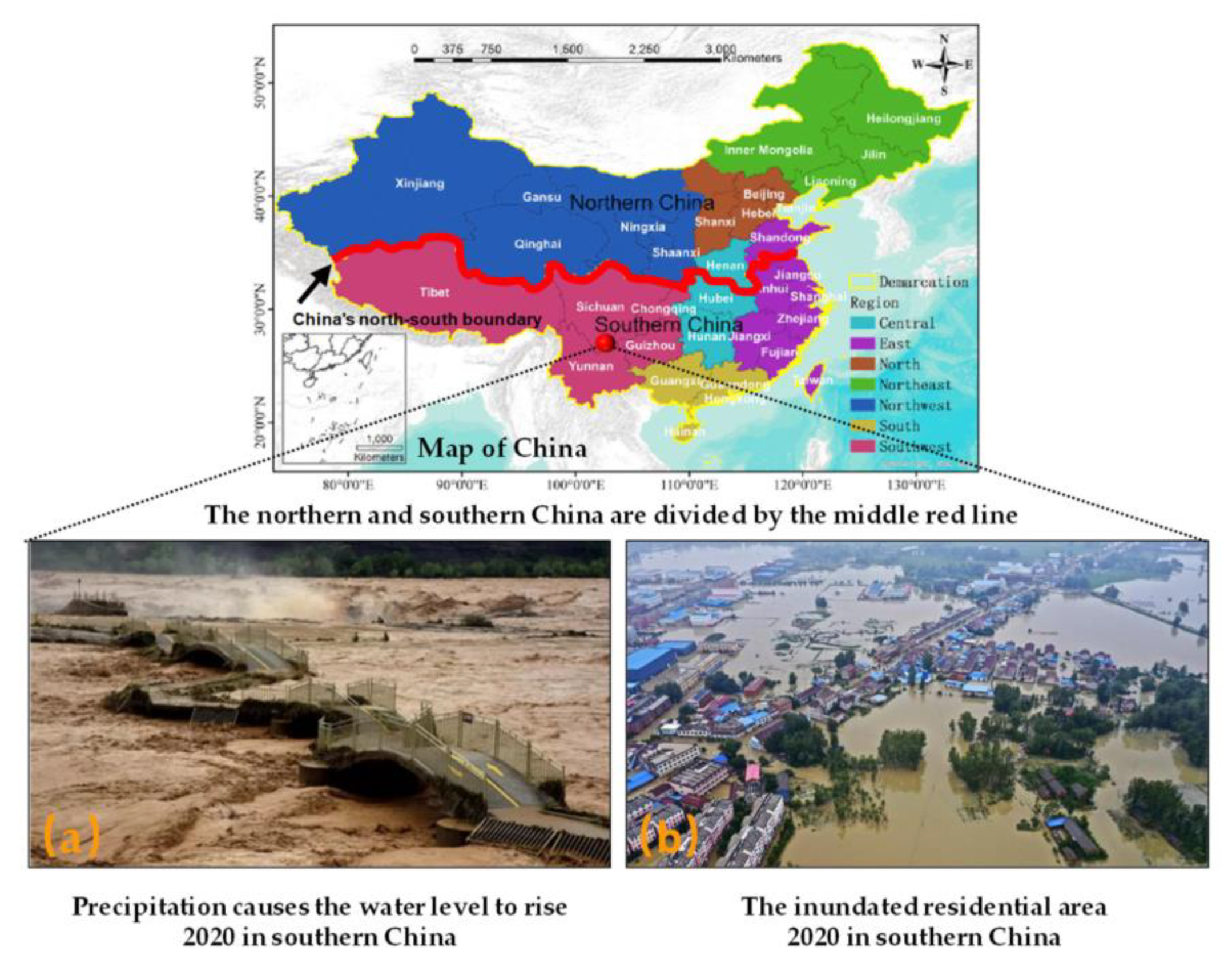
From many historical flood events, it is observed that flood disaster is one of the most frequent and destructive natural disasters [1]. Due to the dual impacts of global climate change and human activities, the frequency of extreme weather has dramatically increased, and large-scale floods have also occurred frequently, bringing vast losses of life and property to people [2]. For example, since the 2020 flood season, precipitation in various parts of Southern China has been expressively higher than in previous years, causing the largest flood disaster since 1998 (shown in Figure 1). The flood disaster was so disastrous that more than 30 million people were affected, 141 people died, and 22,000 houses collapsed. In addition, an economic loss of approximately 60 billion yuan occurred.

Due to the time and resource limitations and rapid changes in the flooding process, it is always a huge challenge to collect information for hazard mitigation promptly, as proper actions must be performed within a limited amount of time. Today, the application of remote sensing for flood studies is receiving considerable attention. The development in this field has evolved from optical to radar remote sensing [3]. Though radar data could provide frequent day and night observations of the surface under almost any weather condition, they have relatively low resolution and high noise. The imaging of radar data cannot provide an intuitive image experience as well. Besides, satellite synthetic aperture radar (SAR) imagery of some urban areas is difficult to interpret because of the off-nadir viewing configuration, for example, the confusion of floodwater with a specular reflection of smooth land surfaces [4]. Optical remote-sensing data are used broadly for regional monitoring and mapping. They have a cost-effective advantage over radar data for flood extent mapping, especially under cloud-free conditions. Optical images are more suitable for studying flood inundation with a relatively long-time span, rapid water rising, and slow retreating, such as "coastal flood" and "fluvial flood". Meanwhile, the bad weather was primarily concentrated in the pre-flood period, and not all of the weather was severe during flooding. A part of the optical remote-sensing image data with relatively good quality was available. Thus, the main objective of the research described in this paper was to develop a decision support system to evaluate the impact of flood hazards based on these limited remote-sensing data in a widely used Geographic Information System (GIS) environment. State agencies need those reliable decision support systems to assess flood loss, plan and design flood management strategies and mitigation systems, and prepare emergency management plans that may involve.

To carry out a flood hazard assessment from remote-sensing imagery, we should first need to identify the water bodies and their distribution from the remote-sensing imagery. The current water information-extraction methods mainly include the threshold method, machine learning method, and deep learning method. The threshold method constructs a model by selecting the appropriate band in the information transmitted from the satellite and uses the different spectral characteristics of water bodies and non-water bodies to extract water bodies [5]. It is divided into the single-band threshold method [6], inter-spectral relationship method, and water-body index method [7,8,9,10], among which the water index method is the most popular. The earliest water index method, named the Normalized Difference Water Index (NDWI), was proposed in 1996 [7], eliminating the interference of some vegetation and soil information to extract water. However, the threshold methods have trouble selecting water bodies from objects with similar spectral features, such as shadows and dark roads. With the development of machine learning, several popular machine learning algorithms, such as Decision Tree (DT) [11,12], Support Vector Machine (SVM) [13,14], and Random Forest (RF) [15,16], have been widely used in water body extraction. However, these methods need to mark features artificially, and different feature vectors are required for changed pictures; the quality of the mark has a significant impact on the results [17]. Traditional methods mainly rely on manually designed extractors, requiring professional knowledge and complicated parameter adjustment processes. Thus, the generalization ability and robustness of these methods need to be improved.

Today, deep learning has become popular in image processing, including remote-sensing images as well. The advantage of convolutional neural network (CNN) is that features could be captured directly from the original images through multiple convolutional layers [18], which avoid complex feature processing. Some models, such as U-Net [19], LinkNet [20], and DeeplabV3+ [21], were popular in the field of image recognition and had relatively good results in terms of accuracy. U-Net was widely used for its simple and straightforward encoding–decoding structure [22]. However, U-Net is poor in edge information extraction and easily misses part of the targets. In addition, water extraction is different from general target extraction, and it has pronounced regional differences. Some surface features with spectral reflectance close to water, such as shadows, roads, dark roofs, etc., can easily interfere with the water extraction results, leading to incorrect mention and omission of deep learning models. To date, most of the water datasets published lacked samples in complex geological environments.

How to generate a continuous and dynamic flood process through the intermittent flood inundation range extracted by the deep learning model still faces significant challenges. To obtain a dynamic and continuous flood inundation process, the flood evolution model that relies on a priori data was often used in hydrology to describe the flood movement process. Those methods could accurately simulate the water level, flow rate, and changes over time by solving hydrodynamic equations. Still, the uncertainty of the parameters due to regional differences reduced the accuracy of the results, especially in areas with insufficient data [23]. Moreover, flood disasters have the characteristics of suddenness, and many disaster-stricken sites could not provide sufficient real-time observational data. Furthermore, remote-sensing data could be used directly to extract information about the extent of flood inundation. It can infer hydrological model parameters by extracting underlying surface features, such as the land cover and impervious area ratio. The data-assimilation method can integrate the observation data information and the constraints of the hydraulic model and use multi-source information to minimize the uncertainty in the flood evolution process [24]. There are two main ways to use hydraulic models to assimilate remote-sensing data. One is to assimilate water-level data extracted from remote-sensing data with hydraulic models [25]. The assimilation effect of this method depends on the accuracy of the extracted water-level data. The accuracy of the data obtained by the current approach is still low and is at the meter level, which is not very compatible with the hydraulic model. On the other hand, the remote-sensing data have a high resolution at present, from which a high-resolution flood inundation range could be obtained. Thus, it is more direct and practical to use the flood-inundation-area data rather than the water-level data to assimilate the flood evolution process. Lai et al. [26] researched the fusion of flood inundation range data and the flood dynamics model to dynamically correct the dynamics model. Zhang et al. [27] transformed the flood inundation process into the topological deformation between the curves of the inundation area and performed numerical solutions from space and time dimensions. However, these models still do not fully satisfy the needs of city emergency management, due to model complexity, setup data requirements, and computing times. Besides, there are still few related studies.

Since the submerged-area data obtained from remote-sensing images contain rich hydraulic spatial information, this paper aimed to develop a robust decision support system for integrated flood inundation management based on limited remote-sensing images. Firstly, we established a water-extraction convolutional neural network to cost-effectively and accurately extract the water body for the first challenge. Specific datasets were used in training the model to separate the water body from the confusing surface features. In addition, we built a waterfront contour active tracking model to implicitly describe the flood movement interface for the second challenge. The spatial upwind difference and time Euler difference methods were used to obtain the numerical solution of the implicit function and interpolate the submerged range in time and space. Finally, we developed a decision support system, using ArcGIS API. The decision support system combined fast raster layer operations in the GIS platform with vulnerability models to generate flood-hazard maps for decision-makers.

The structure of the rest of this article is as follows. First, we introduce the basic principles of the proposed models. Secondly, we report how we tested and evaluated the performance of the models on a laboratory scale. Simultaneously, we took the Chaohu Lake basin, Anhui Province, as the study area to verify the actual capabilities of the models. The daily inundation ranges from June 15 to September 30 during the flooding process were simulated from the limited raw imagery. Finally, we packaged the models above to develop an information system for loss assessment. The validation of the evaluation results was carried out by cross-comparison.

2. Methodology

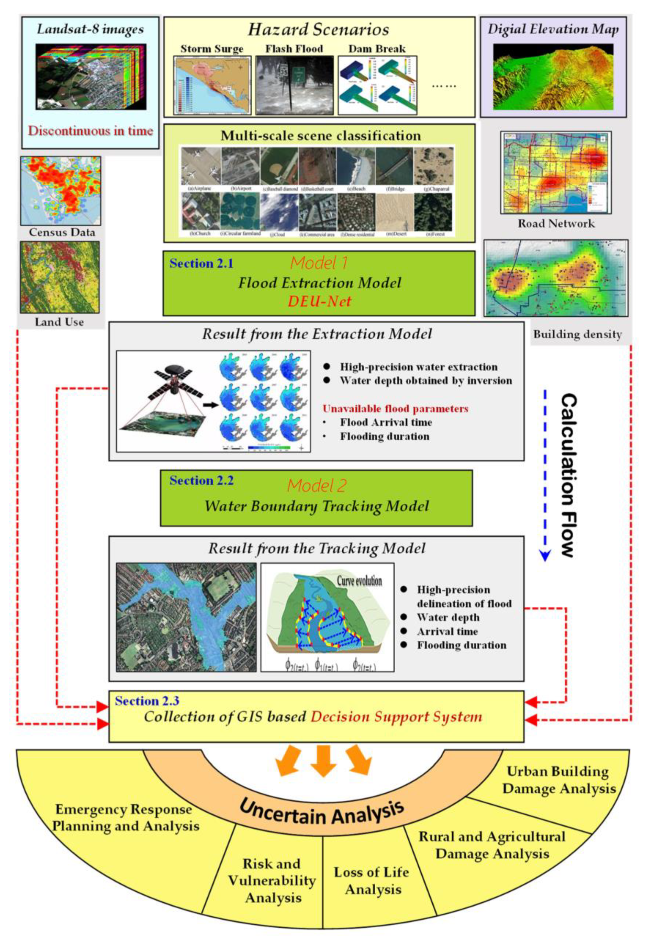
The model proposed in this paper was divided into three parts: multi-scale flood-information-extraction model, water-boundary tracking model, and loss-assessment decision support system, as shown in Figure 2.

2.1. Multi-Scale Flood-Information-Extraction Model

To fully use the cost-effective optical remote-sensing data, we expected to establish a model to extract visible floodwater by using RGB band digital numbers to obtain an accurately distributed water extent with a relatively high spatial resolution.

2.1.1. Model Design

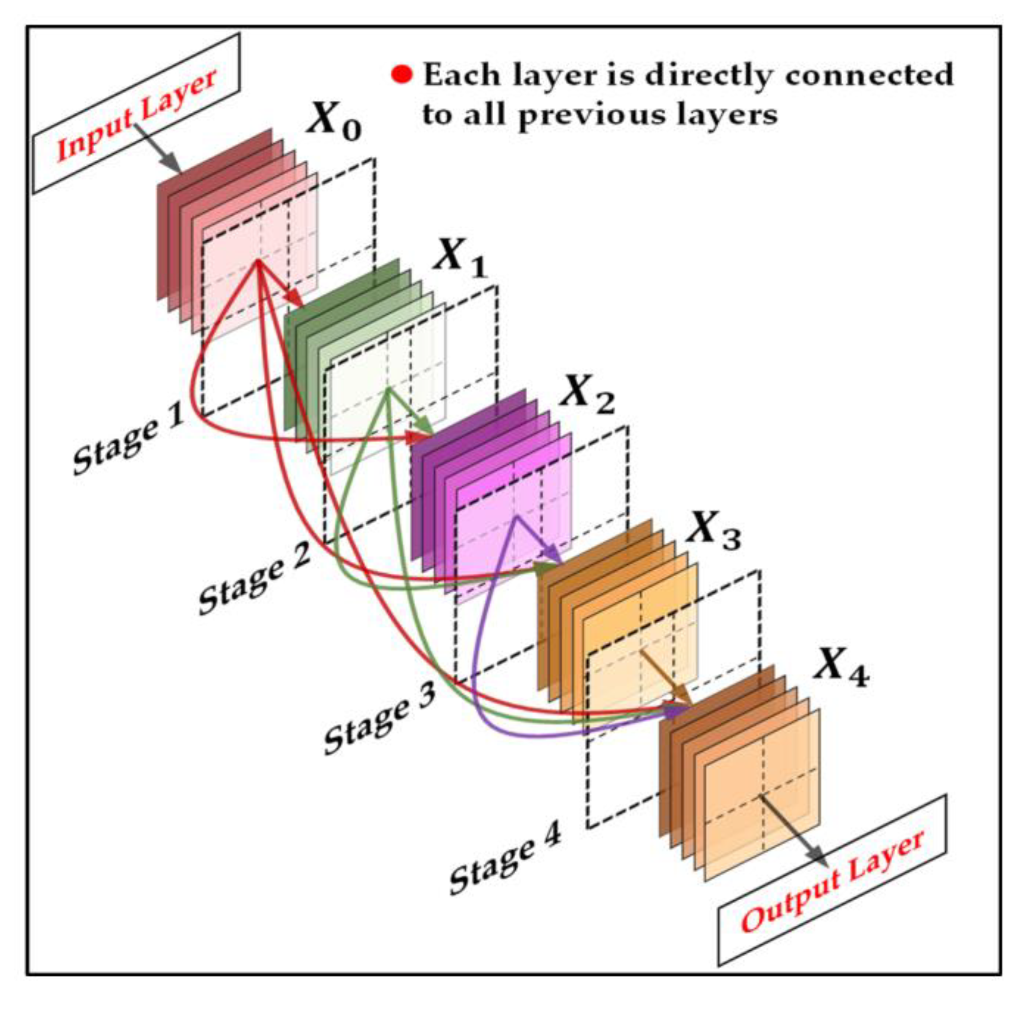
The multi-scale flood information extraction model called DEU-Net proposed in this paper combines the advantages of U-Net and DenseNet. It replaces the ordinary convolution module used for feature extraction in the original structure of U-Net with densely connected blocks in DenseNet. U-Net is an encoding–decoding network based on a fully convolutional neural network and is composed of a symmetrical down-sampling process and an up-sampling process [22]. U-Net combines the information obtained from the downsampling process and the information input from the up-sampling process to restore the details of images [28]. DenseNet [29] is a convolutional neural network with dense connections. There is a direct connection between any two layers in DenseNet. The input of each layer in the network structure is the union of the outputs of all the previous layers, and the feature maps obtained from this layer will also be directly passed to all subsequent layers as input information [30]. The structure of the dense connection block is shown in Figure 3. This structure could fuse information from multiple scales to obtain more affluent and adequate information, thus enhancing the network’s expressive capability. In addition, since the sources of our datasets were public datasets, Landsat-8 and GF-1, water bodies in our dataset had multi-scale features due to the gradual improvement in resolution [31]. After training on the datasets, the multi-scale flood-information-extraction model could fully extract a small area of water and keep the integrity of the slender river, which performs well in dig-out water from remote-sensing images.

In the down-sampling feature extraction part of the structure, the images were resampled to a pixel resolution of 512 × 512 as input. First, the input passed through 64 filters of size 3 × 3 to obtain an initial feature map of 256 × 256 × 64 and then entered the Dense Block to extract the feature. Since the characteristics of water bodies in remote-sensing images were apparent, each Dense Block set the number of layers $L$to 3 and the growth rate $k$ to 12 to reduce graphics processing unit (GPU) consumption during model training. Each dense layer contained a convolutional layer of size 3 × 3, a batch normalization (BN) layer, and a rectified linear unit (ReLU) layer. A transition layer connected every two Dense Blocks. Each transition layer had the same structure and consisted of a bottleneck layer with a filter of size 1 × 1, an average pooling layer of size 2 × 2, and a dropout layer. Then the input image passed through 5 Dense Blocks and four down-sampling transition layers during the down-sampling process on the left of the model structure. The feature map output by the fifth Dense Block was of size 16 × 16 and then went in the up-sampling expansion stage on the right. The structure on the right was similar to the structure on the left. It was composed of 4 transition layers and 5 Dense Blocks. The role of the transition layer was to deconvolute and expand the abstract feature map obtained by feature extraction by using a 3 × 3 filter. While performing up-sampling, feature maps of the same size on the left and right sides were merged through jump connections. This design improved the utilization of feature information and provided more gradient flow information, thus enhancing the network structure’s training performance and training speed.

2.1.2. Sample Generation

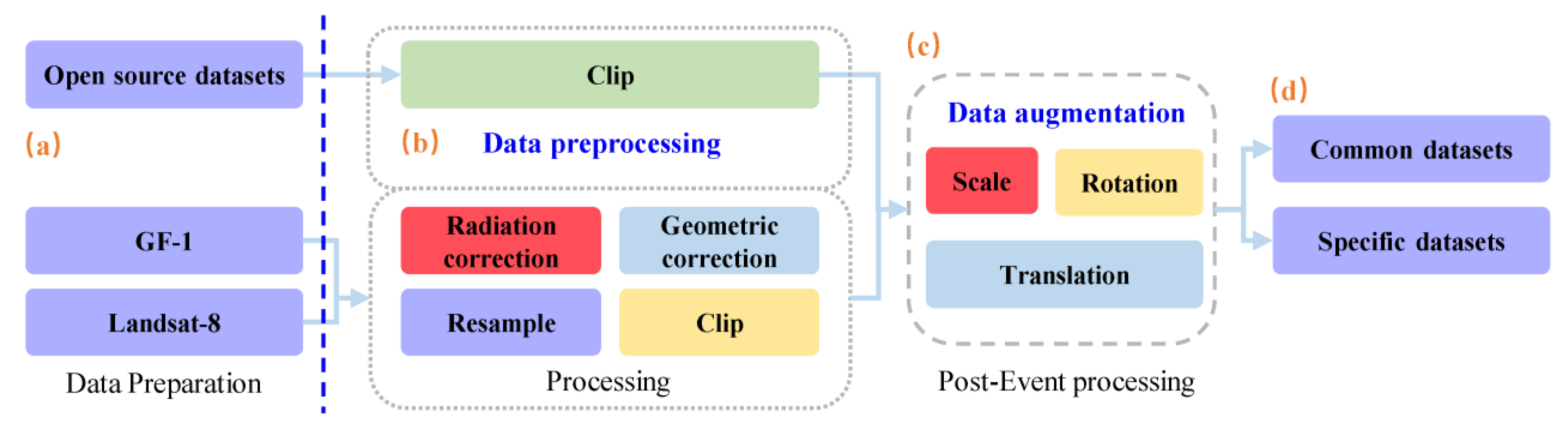
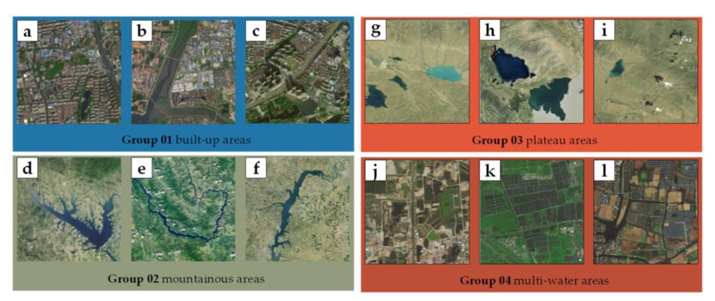
Due to the distinct discrepancies in the water features and the surrounding environment in different regions, the accuracy of the extraction results obtained by the same model may also be uneven. If the model was only trained by standard datasets, it was tough to get good extraction results when the surrounding environment was relatively unsophisticated. Therefore, in addition to making universal water datasets based on Landsat-8 OLI and Gaofen-1 (GF-1) satellite data, we collected images of water bodies in various regions of our country based on Landsat-8 OLI and performed detailed analysis and classification. Regarding the nature of the water body and the confusion of surface objects, the research fields with complex conditions were divided into four typical types. We trained the common datasets and then performed the corresponding specific datasets to get the specific model at first. Before starting water-extraction work, the kind of research area involved should be roughly judged. If the terrain condition is simple, we could use the model trained by standard datasets. If the circumstance is complex, we should first determine which feature area is closer and selected the corresponding model for water body information extraction. The generation process of the datasets is shown in Figure 4, and some samples in specific datasets are shown in Figure 5.

The specific datasets were divided into four typical regions:

• Built-up areas: the shapes of water bodies in built-up areas are relatively regular, mainly natural or artificial rivers and lakes. However, the surface features are somewhat complex, and there are several confusing features, such as building shadows, roads, dark lawns, and dark roofs [17].
• Mountainous areas: The water bodies in mountainous areas are primarily rivers. Mountain rivers have many branches, and it is hard to accurately extract the edges for the most part. Moreover, they are easily confused with mountain shadows.
• Plateau areas: The chief water bodies in the plateau areas are plateau lakes and plateau rivers. Because of their rich mineral ions, the colors of the water bodies are different from the common ones, such as turquoise and light blue. Confusing features are mountain shadows and cloud shadows left in the image due to the shooting angle.
• Multi-water areas: These areas contain rich water resources, mainly in farming regions such as paddy fields and fish ponds. The water bodies in this area are compactly distributed with many types and different scales. They may include lakes, rivers, and ponds, as well as small puddles. Ground objects that are easy to confuse include farmland and masking nets. In the low resolution of remote-sensing images, water bodies may be indistinguishable from dark farmland.

2.2. Water Boundary Tracking Model

The results obtained in the previous section have a high spatial resolution but a low temporal resolution. To receive a flooding process with a high resolution in both time and space, we expected to develop a model to dig out the dynamic and continuous process of flood extent change based on the obtained flood extraction results.

2.2.1. Curve Evolution

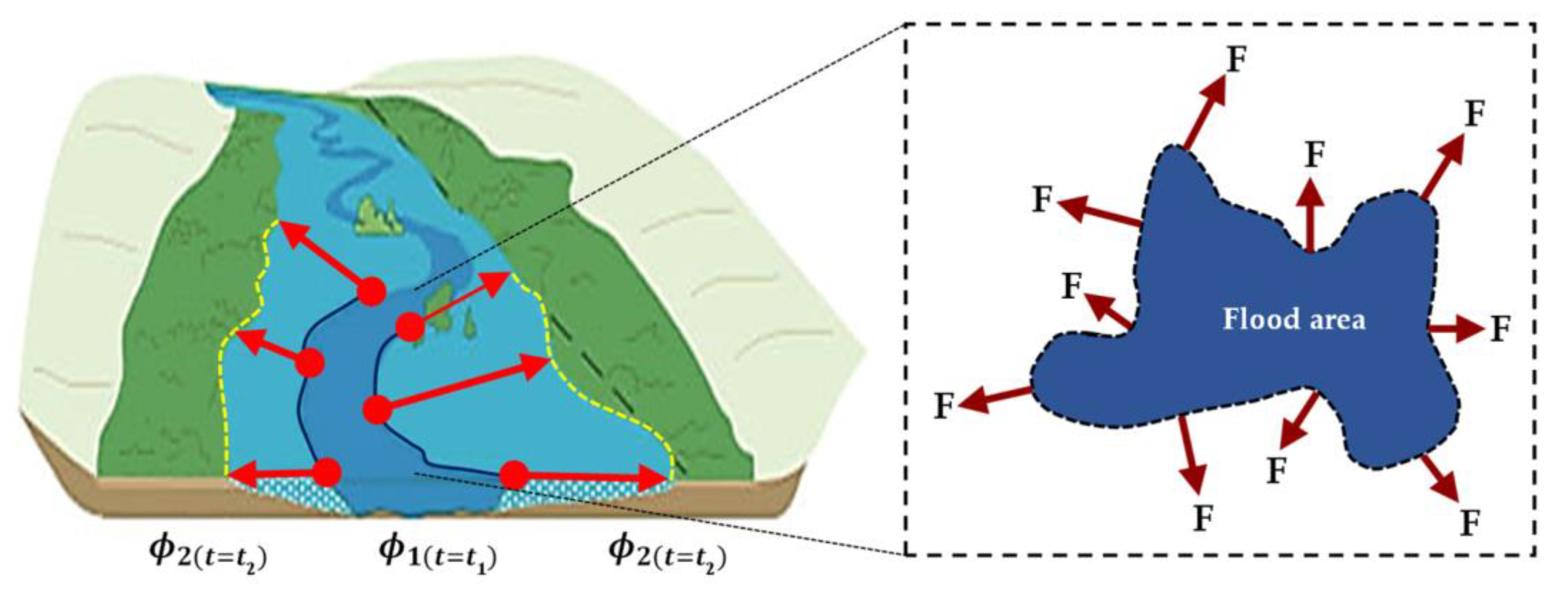
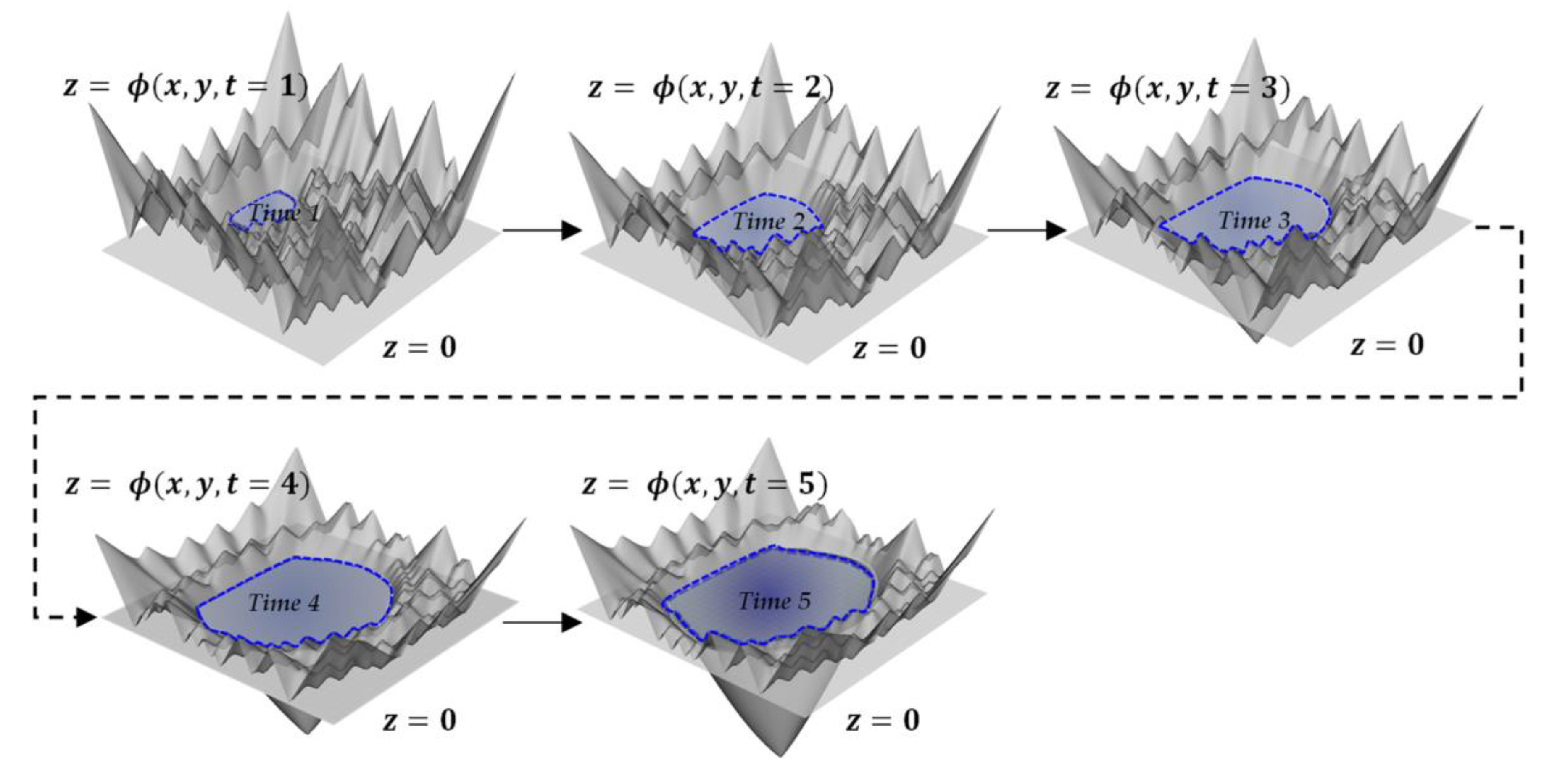
The active boundary tracking method is an effective tool for processing the topological changes of the motion curve with time, based on techniques of curve evolution. The problem becomes the "mean-curvature flow"—similar to evolving active contour, it will stop on the expected boundary. We presented a numerical algorithm by using finite differences. This method describes the continuous function $\varphi \left(x,y,t\right):R^3\to R$ as the implicit expression of a closed evolution curve $C\left(p,t\right):0⩽p⩽1$ at time t. That is, the curve $\mathrm{C}\left(p,t\right)$ at time t corresponds to the zero-level set of $\varphi \left(x,y,t\right)$. In this paper, the flood inundation range at time $t_1$ was the source surface ${\varphi }_1$, and the flood inundation range at time $t_2$ was the target surface ${\varphi }_2$ $\left(t_1<t_2\right)$. Thus, the evolution process of the flood inundation range was transformed into the process of ${\varphi }_1$ infinitely approaching ${\varphi }_2$ under the control of partial differential equations (see Figure 6).

2.2.2. Mathematical Derivation of the Model

Let $\Omega$ be a bounded open subset of ${ℝ}^2$ with $\partial \Omega$its boundary. Let $u_0: \overline{\mathsf{\Omega }} \to ℝ$ be a given area, and $C\left(s\right):\left[0,1\right]\to {ℝ}^2$ be the parameterized evolving curve in $\Omega$, as the boundary of an open subset $\mathsf{\omega }$ of $\Omega$. In what follows, $inside\left(C\right)$ denotes the region $\mathsf{\omega }$, and $outside\left(C\right)$ denotes the $\Omega \setminus \overline{\omega }$. Assume that the area is formed by two regions of approximatively piecewise-constant intensities, of distinct values $u_0^i \mathrm{and} u_0^o$, representing the flooded area and the un-inundated area. Suppose further that the object to be detected is represented by the area with the value $u_0^i$. Let denote its boundary by $C_0$. Then we have inside the object [or $inside \left(C_0\right)$], and outside the object [or $outside \left(C_0\right)$]. Let us now consider the following “fitting” term:

$$\begin{array}{ll}{F}_1(C)+F_2(C)=& {{\displaystyle \int }}_{\text{inside}(C)}{\left|u_0(x,y)-c_1\right|}^{2}dxdy\\ & +{{\displaystyle \int }}_{\text{outside}(C)}{\left|u_0(x,y)-c_2\right|}^{2}dxdy,\end{array}$$

(1)

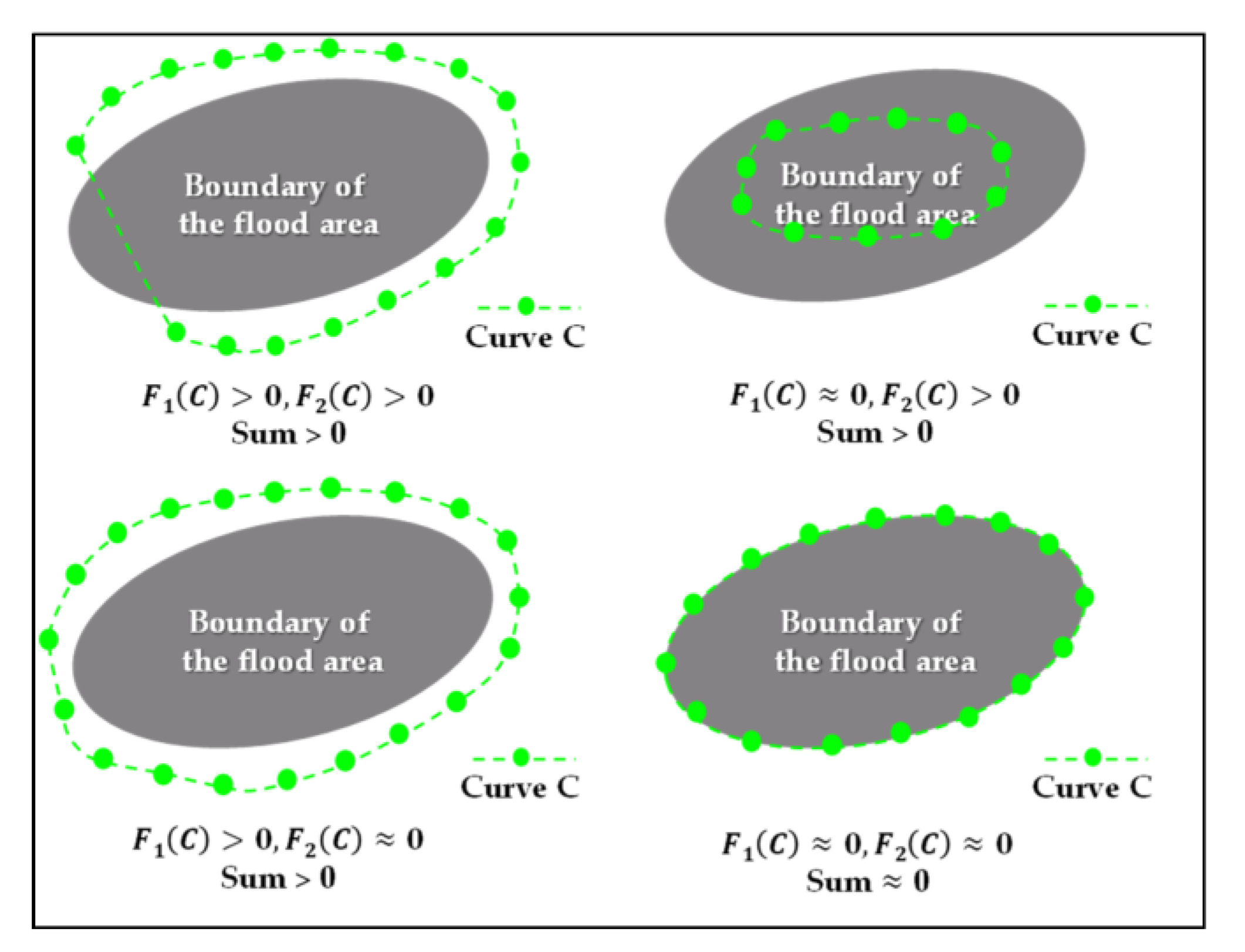
where $C$ is any closed curve, and the constants $C_1 \mathrm{and} C_2$, depending on $C$, are the averages of $u_0$ inside and outside, respectively. It is obvious that $C_0$, the boundary of the object, is the minimum value of the fitting term, as shown in Figure 7.

In addition, we added some regularizing terms, such as the length of the curve and the region’s area inside. We introduced the energy functional $F\left(c_1,c_2,C\right)$, which is defined as follows:

$$\begin{array}{cc}F\left(c_1,c_2,C\right)=\mu \cdot & Length(C)+v\cdot Area(inside(C))+{\lambda }_1{{\displaystyle \int }}_{\text{inside}(C)}{\left|u_0(x,y)-c_1\right|}^{2}dxdy\\ & +{\lambda }_2{{\displaystyle \int }}_{\text{outside}(C)}{\left|u_0(x,y)-c_2\right|}^{2}dxdy,\end{array}$$

(2)

where $\mu \ge 0,\nu \ge 0,{\lambda }_1, \mathrm{and} {\lambda }_2>0$ are fixed parameters. $Length\left(C\right)$ is the length of the closed contour line C, $Area\left(inside\left(C\right)\right)$ is the internal area of $C$, and ${\lambda }_1$ and ${\lambda }_2$ are the weight coefficients of each energy term. In almost all of our numerical calculations (see further), we fix ${\lambda }_1={\lambda }_2$. Therefore, we considered the minimization problem: $\underset{c_1,c_2,C}{\mathit{inf}}F\left(c_1,c_2,C\right)$

We sought the best approximation of the function that took only two kinds of values, namely $u=\{\begin{array}{l}\mathrm{u}<0 \mathit{inside} C\\ \mathrm{u}\text{>}0 \mathit{outside} C\end{array}$. The initialization of the function u is simple for the regular initial contour, and the curve C we selected is a normal circle with a center $\left(x_0,y_0\right)$ and a radius of r. The calculation formula of the function u is $u_0\left(x,y\right)=\sqrt{{\left(x-x_0\right)}^2+{\left(y-y_0\right)}^2}-r$. Then, using the Heaviside function $H$ and the one-dimensional Dirac measure, ${\delta }_0$, defined by $H\left(z\right)=\{\begin{array}{c}1,\text{ if }z\ge 0\\ 0, \text{if }z<0\end{array}$ and ${\delta }_0\left(z\right)=\frac{d}{dz}H\left(z\right)$, we expressed the terms in the energy in the following way:

$$\begin{array}{ll}F\left(c_1,c_2,\varphi \right)=\mu & {{\displaystyle \int }}_{\text{Ω}}\delta (\varphi (x,y))|\nabla \varphi (x,y)|dxdy+v{{\displaystyle \int }}_{\text{Ω}}H(\varphi (x,y))dxdy+{\lambda }_1{{\displaystyle \int }}_{\text{Ω}}{\left|u_0(x,y)-c_1\right|}^{2}H(\varphi (x,y))dxdy\\ & +{\lambda }_2{{\displaystyle \int }}_{\text{Ω}}{\left|u_0(x,y)-c_2\right|}^2(1-H(\varphi (x,y)))dxdy,\end{array}$$

(3)

Keeping $\varphi$ fixed, with respect to the constants and $c_2$, it is easy to express these constants’ function of by using the following:

$$c_1\left(\varphi F\left(c_1,c_2,\varphi \right)\right)=\frac{{{\displaystyle \int }}_{\text{Ω}}{u}_0(x,y)H(\varphi (x,y))dxdy}{{{\displaystyle \int }}_{\text{Ω}}H(\varphi (x,y))dxdy},$$

(4)

$$c_2(\varphi )=\frac{{{\displaystyle \int }}_{\text{Ω}}{u}_0(x,y)(1-H(\varphi (x,y)))dxdy}{{{\displaystyle \int }}_{\text{Ω}}(1-H(\varphi (x,y)))dxdy}$$

(5)

By the previous formulas, we saw that the energy $F\left(c_1,c_2,\varphi \right)$ could be written the only function of $H\left(\varphi \left(x,y\right)\right)$. Keeping $c_1$ and $c_2$ fixed, and minimizing $F\left(c_1,c_2,\varphi \right)$ with respect to $\varphi$, we deduced the associated Euler–Lagrange equation for $\varphi$. Parameterizing the descent direction by an artificial time $t\ge 0$, we realized the dynamic evolution of the level set function.

$$\begin{gathered} \frac{\partial \varphi }{\partial t}=\delta \left(\varphi \right)[\mu div\left(\frac{\nabla \varphi }{\left|\nabla \varphi \right|}\right)-\nu -{\lambda }_1{\left(u_0-c_1\right)}^2+{\lambda }_2{\left(u_0-c_2\right)}^2] \\ =0 \mathrm{in} \left(0,\infty \right)\times \Omega , \end{gathered}$$

(6)

$$\frac{\delta \left(\varphi \right)}{\left|\nabla \varphi \right|}\frac{\partial \varphi }{\partial \overrightarrow{n}}=0 \mathrm{on} \partial \Omega ,$$

(7)

To discretize the equation in $\varphi$, we used a finite differences implicit scheme. Firstly, we recalled the usual notations: let $h$ be the space step, $\Delta t$ be the time step, $\left(x_i,y_j\right)=\left(ih,jh\right)$ be the grid points, and ${\varphi }_{i,j}^n=\varphi \left(n\mathsf{\Delta }t,x_i,y_j\right)$ be an approximation of $\varphi \left(t,x,y\right)$. To ensure the accuracy of the solution and avoid numerical dissipation, the spatial upwind difference format and the time Euler difference format were selected for discretization. The finite differences are as follows:

$${\mathsf{\Delta }}_{-}^x{\varphi }_{i,j}={\varphi }_{i,j}-{\varphi }_{i-1,j},$$

(8)

$${\mathsf{\Delta }}_{+}^x{\varphi }_{i,j}={\varphi }_{i+1,j}-{\varphi }_{i,j},$$

(9)

$${\mathsf{\Delta }}_{-}^y{\varphi }_{i,j}={\varphi }_{i,j}-{\varphi }_{i,j-1},$$

(10)

$${\mathsf{\Delta }}_{+}^y{\varphi }_{i,j}={\varphi }_{i,j+1}-{\varphi }_{i,j}.$$

(11)

where ${\mathsf{\Delta }}_{+}^x{\varphi }_{i,j}$ and ${\mathsf{\Delta }}_{-}^x{\varphi }_{i,j}$ represent the forward difference format and backward difference format in the x-direction, respectively. ${\mathsf{\Delta }}_{+}^y{\varphi }_{i,j}$ and ${\mathsf{\Delta }}_{-}^y{\varphi }_{i,j}$ represent the forward and backward difference formats in the y-direction. The discretization of the divergence operator and the iterative algorithm is as follows. Knowing ${\varphi }^n$, we first computed $c_1\left({\varphi }^n\right) \mathrm{and} c_2\left({\varphi }^n\right)$. Then, we computed ${\varphi }^{n+1}$ by the following discretization and linearization.

$$\begin{gathered} \begin{array}{c}\frac{{\varphi }_{i,j}^{n+1}-{\varphi }_{i,y}^n}{\text{Δ}t}={\delta }_n\left({\varphi }_{ij}^n\right)[\frac{\mu }{h^2}{\text{Δ}}_{-}^x\cdot \left(\frac{{\text{Δ}}_{+}^x{\varphi }_{l,f}^{n+1}}{\sqrt{{\left({\text{Δ}}_{+}^x{\varphi }_{ij}^n\right)}^2/\left(h^2\right)+{\left({\varphi }_{i,j+1}^n-{\varphi }_{h,j-1}^n\right)}^2/{(2h)}^2}}\right)\\ .\end{array} \\ +\frac{\mu }{h^2}{\text{Δ}}^y\cdot \left(\frac{{\text{Δ}}_{+}^y{\varphi }_{i,j}^{n+1}}{\sqrt{{\left({\varphi }_{i+1,f}^n-{\varphi }_{i-1,j}^n\right)}^2/{(2h)}^2+{\left({\text{Δ}}_{+}^y{\varphi }_{i,j}^n\right)}^2/\left(h^2\right)}}\right)-v-{\lambda }_1{\left(u_{0,i,j}-c_1\left({\varphi }^n\right)\right)}^2+{\lambda }_2{\left(u_{0i,l}-c_2\left({\varphi }^n\right)\right)}^2] \end{gathered}$$

(12)

When the implicitly expressed function ${\varphi }_{i,j}^t$ was used for surface evolution, the zero isosurface $\mathrm{C}\left(t\right)=\left\{\left(i,j\right)\in \mathsf{\Omega }:{\varphi }_{i,j}^t=0\right\}$ of the function was the evolving shape of the flood inundation range at that point in time t.

2.3. Decision Support System for Integrated Flood-Loss Assessment

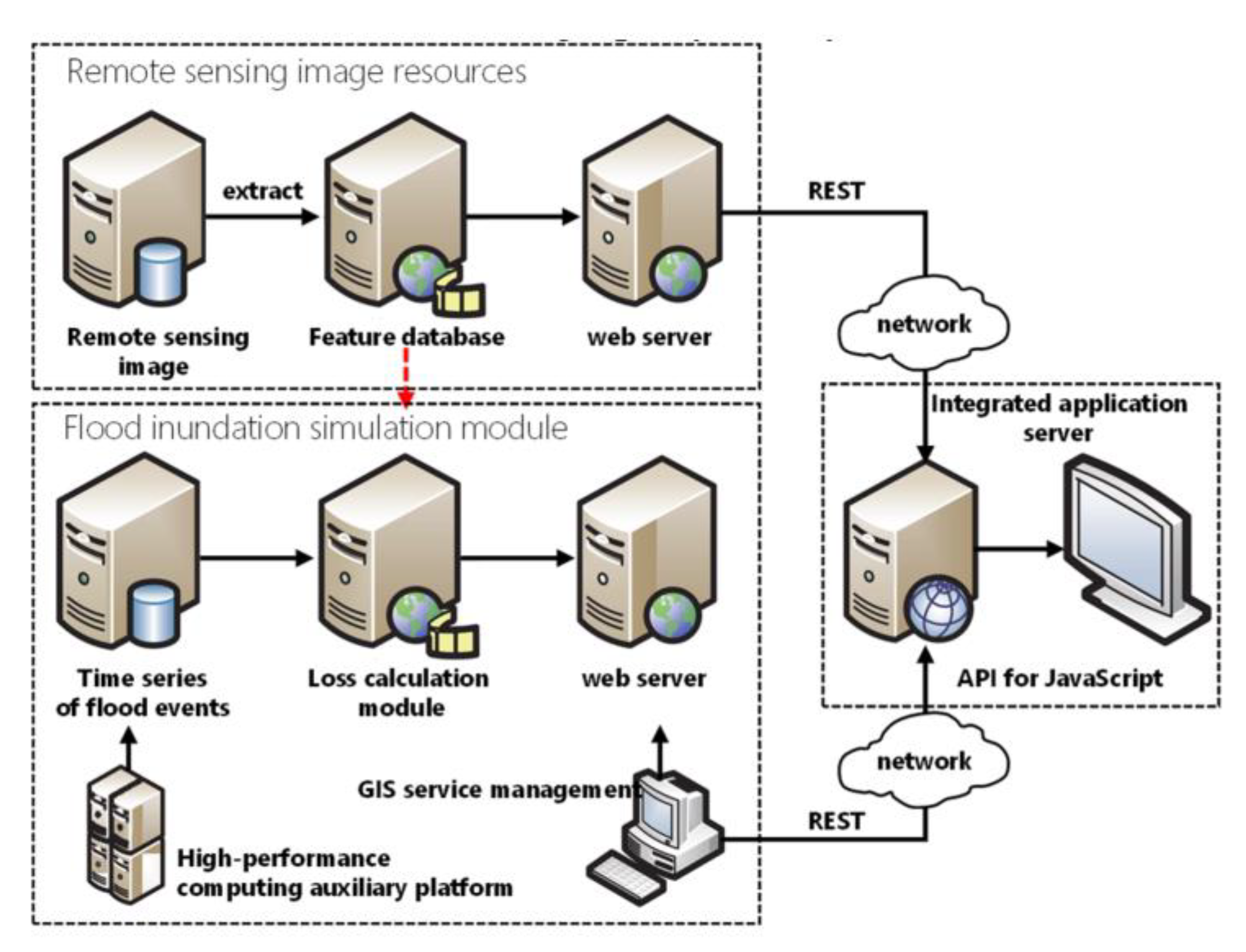
The final task of this research was to develop an innovative decision support system for integrated flood-loss assessment that allows for a detailed evaluation of the consequences of a flood event. A collection of GIS-based decision-support modules constitutes the core of the proposed system [32]. The previous model provides information about the extent of the flooded area, spatial distributions of flood depth, the arrival time of the flood, and its duration at each point of the computational domain. To carry out these tasks, we need to complement the GIS decision support system with various geospatial information, such as land use, census data, building density, and road network [33]. The system mainly includes the following aspects: remote-sensing image, vector-element resources, flood-inundation data, loss-calculation model, and client implementation, as shown in Figure 8. We used the high-performance platform to obtain the flood inundation data of the computing area and utilized the data conversion tool to convert the data into the corresponding time-series layer. All data were provided to the client in representational state transfer (REST) transmission format. The client used the integrated application server to aggregate data from different sources and realized functions such as browsing, query, analysis, and calculation.

To accurately and rapidly evaluate the risk of flood inundation, we selected the cloud model to assess the flood disaster loss and used the entropy weight method to calculate the weight of each indicator. The cloud model [34] is a fuzzy mathematics method based on the uncertainty of concepts in natural language, which starts from the connection between ambiguity and randomness, and realizes the uncertain conversion between qualitative concepts and their quantitative values. The cloud is composed of disordered cloud drops, and a cloud drop means the quantitative realization of a qualitative concept. The more cloud drops, the more it could symbolize the characteristics of the qualitative concept. The main parameters of the cloud model are the expectation ($E_x$), the entropy ($E_n$), and the hyper-entropy ($H_e$). Forward Cloud Generator is the most popular among the cloud models, and it was used in this study. After obtaining the certainty degrees of different indicators through the Forward Cloud Generator, we used the entropy weight method [35] to calculate the weight of each indicator in the flood-disaster loss assessment. The detailed computational flow of the cloud model is presented in

Table A1. The risk calculation process of the cloud models embedded in the system.

Input	Steps	Output
$1. \mathrm{Digital} \mathrm{Features}$ $({\mathrm{E}}_x$, ${\mathrm{E}}_n$, ${\mathrm{H}}_e$) 2. The number of cloud drops $N$	① Create a normal random number $E_n^{\prime }$ with ${\mathrm{E}}_n$ as the expected value and $H_e^2$ as the variance.	$\mathrm{Drop}\left(x_i,{\mu }_i\right)$
	② Create a normal random number $x_i$ with ${\mathrm{E}}_x$ as the expected value and $E_n^{\prime }{}^2$ as the variance.
	③ Calculate the certainty degree ${\mu }_i=e^{\frac{-{\left(x_i-{\mathrm{E}}_x\right)}^2}{2{\left(E_n^{\prime }\right)}^2}}$
	④ Generate a cloud drop with ${\mu }_i$ and $x_i$.
	⑤ Repeat steps 1~4 until the number of cloud drops reaches $N$
$3. \mathrm{The} \mathrm{number} \mathrm{of} \mathrm{objects} m$ 4. The number of indicators $n$	⑥ Calculate the proportion of each indicator $f_{ij}=\frac{1+x_{ij}}{n+{{\displaystyle \sum }}_{j=1}^n{x}_{ij}}$ (i and j represent the serial number of the objects and indicators, respectively)	$\mathrm{The} \mathrm{weight} \mathrm{matrix}, W$
	⑦ Calculate the entropy value of each indicator $e_i=-\frac{1}{\ln m}{\displaystyle \sum }_{j=1}^m{f}_{ij}\ln f_{ij}$
	⑧ Obtain the weight of each indicator $w_{i }=\frac{1-e_i}{n-{{\displaystyle \sum }}_{i=1}^n{e}_i}$

in Appendix A.

3. Model Performance Testing and Discussion

A laboratory environment was constructed to benchmark the performance of the model and the accuracy of the simulations. The purpose of doing this is that the laboratory environment is manageable and the observational data obtained are more accurate.

3.1. Performance Comparison of the Water Extraction Model Technologies

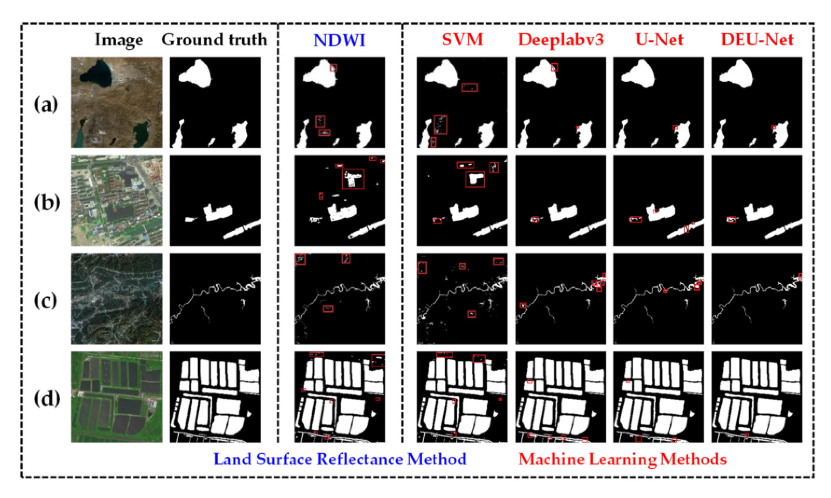
To evaluate the performance of the model DEU-Net, we made a qualitative and quantitative comparison with the traditional method NDWI based on land-surface reflectance and the machine-learning method SVM, and two widely used deep-learning models, U-Net and DeeplabV3+. Qualitative evaluation was to visualize the water-extraction results produced in five typical ways and compare the performance of these methods from visual interpretation. The overall accuracy (OA), the false water rate (FWR), the missing water rate (MWR), and the mean intersection over union (MIoU) were used in the quantitative assessment. The formulas are listed in

Table 1. Four evaluation metrics for accuracy assessment of the identified outcomes.

Evaluation Index	Definition	Formula
OA	The ratio to quantify the degree of match between the predicted value and the actual value	$\mathrm{OA}=\frac{\mathrm{TP}+\mathrm{TN}}{\mathrm{TP}+\mathrm{FP}+\mathrm{FN}+\mathrm{TN}}\times 100\%$
FWR	The ratio of the number of pixels misclassified as water and the number of predicted water pixels	$\mathrm{FWR}=\frac{\mathrm{FP}}{\mathrm{TP}+\mathrm{FP}}\times 100\%$
MWR	The ratio of the number of water pixels that are not recognized as water and the number of actual water pixels	$\mathrm{MWR}=\frac{\mathrm{FN}}{\mathrm{TP}+\mathrm{FN}}\times 100\%$
MIoU	The average of the intersection and union of each type of predicted and actual value	$\mathrm{MIoU}=\frac{1}{2}\left(\frac{\mathrm{TP}}{\mathrm{TP}+\mathrm{FP}+\mathrm{FN}}+\frac{\mathrm{TN}}{\mathrm{TN}+\mathrm{FP}+\mathrm{FN}}\right)$

TP, TN, FN, and FP represent the numbers of pixels of actual water, factual background, false background, and false water, respectively.

.

The results of the water-body extraction using different methods on the test images are shown in Figure 9, and the consequences of accuracy analysis are shown in

Table 2. Comparison of the overall identification accuracy of different models for water bodies.

Method	OA	FWR	MWR	MIoU
NDWI	0.8769	0.1773	0.0690	0.7807
SVM	0.9216	0.0972	0.0607	0.8546
DeeplabV3+	0.9566	0.0578	0.0310	0.9168
U-Net	0.9620	0.0396	0.0382	0.9267
DEU-Net	0.9730	0.0303	0.0245	0.9473

.

As can be seen that NDWI based on land surface reflectance had a humble ability to distinguish between shadows and water bodies, and it was easy to cause false extraction (Figure 9a–c), especially in the built-up area with dense buildings (Figure 9b). In the mountainous area (Figure 9c), the NDWI method confused mountain shadows with water bodies, and the extraction results of tributaries were poor. In the water-rich place (Figure 9d), large-area water bodies had good extraction results, but tiny rivers were difficult to extract accurately. The outcomes extracted by the SVM method had severe noise problems, especially in the built-up area (Figure 9b) and the multi-water area (Figure 9d).

DeeplabV3+, U-Net, and DEU-Net all belong to deep learning methods. These three methods were generally better than the water spectral indices and SVM methods according to their performances. In the plateau area, except for a small part of snow that DeeplabV3+ correctly mentioned, these three methods had little difference (Figure 9a). Moreover, they were good at distinguishing the shadow of the building and the water bodies (Figure 9b). However, as the water body in the lower-left corner was rich in aquatic plants, these three deep learning methods all had a certain degree of error extraction, among which DEU-Net had the lowest degree. In addition, a small part of the water bodies adjacent to the bridge was omitted when using U-Net. DeeplabV3+ had much false extraction in the mountainous area, which confused mountain shadows with water bodies (Figure 9c). In the multi-water area, several dark lands were confused with the water bodies by DeeplabV3+, and the phenomenon of over-extraction was serious. U-Net had two apparent omissions in the lower-left corner, and the results of DEU-Net were the best (Figure 9d).

According to the results of the accuracy analysis shown in Table 2, DEU-Net performed better than the others in all four indicators, and NDWI performed worst. As one of the best models for semantic segmentation, DeeplabV3+, performed poorly in FWR in this study but slightly better in MWR. Combined with U-Net, it appeared that DeeplabV3+ was easy to perform overfitting when training for water extraction. The accuracy analysis confirmed the performance of the DEU-Net proposed in this paper.

3.2. Laboratory-Scale Experiment of Dike Flood Boundary Simulation

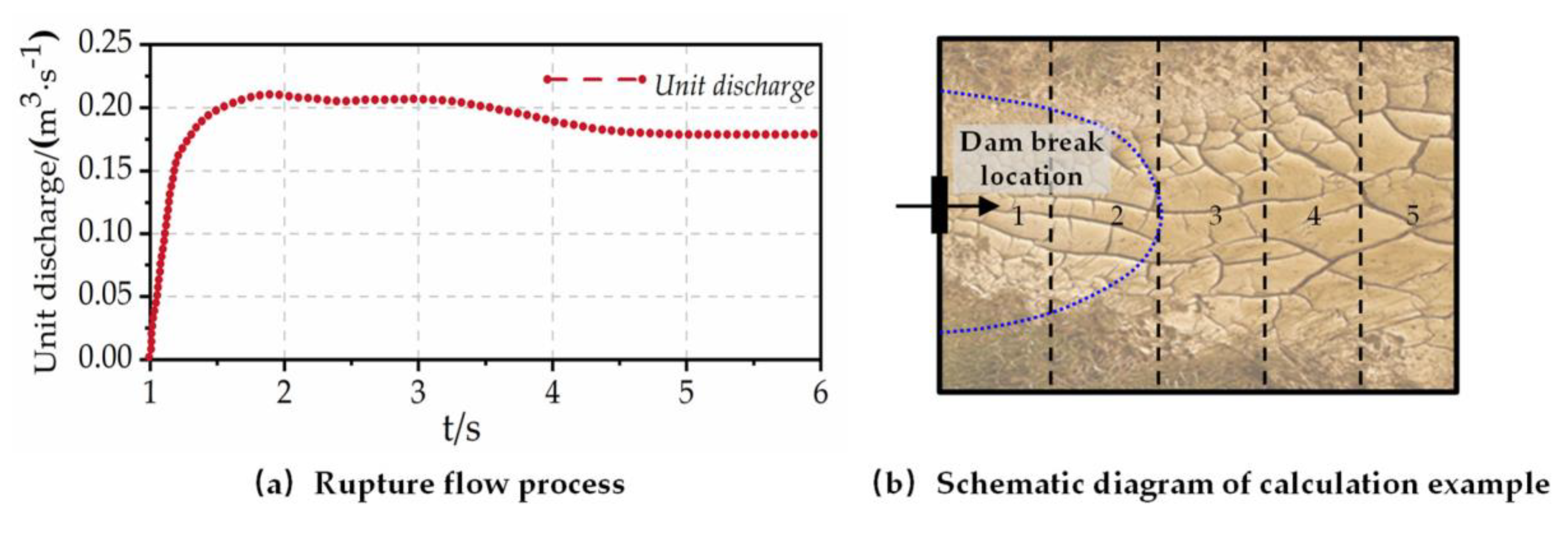
This experiment was a laboratory-scale dike breach process. The calculation area was a rectangular flat-bottomed beach of 10.0 m × 8.0 m, shown in Figure 10a. Five different land-use types were evenly distributed in the study area from left to right, the roughness of which was 0.03, 0.04, 0.05, 0.06, and 0.07, respectively. Assuming that the water flow entered the beach from a fixed breach with a width of 0.4 m from the left-center, the flow process at the fracture boundary is shown in Figure 10b. The duration of the breach was 5 s.

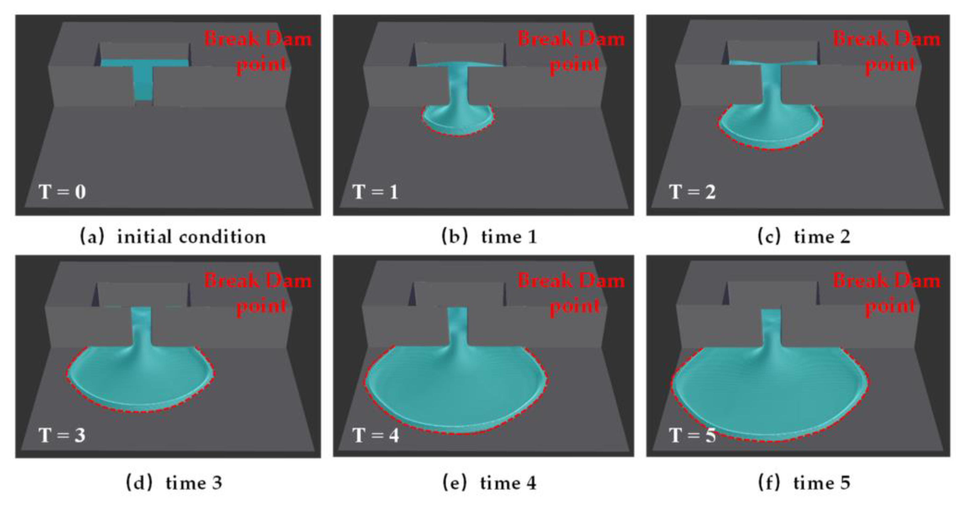
We used the observational data and the results calculated by the 2D hydrodynamic model by using the above-assumed parameters to carry out model verification experiments, as shown in Figure 11. The advantage was that it could deduct the interference of factors, such as the observation and experiment errors, and it was suitable for verifying the proposed model.

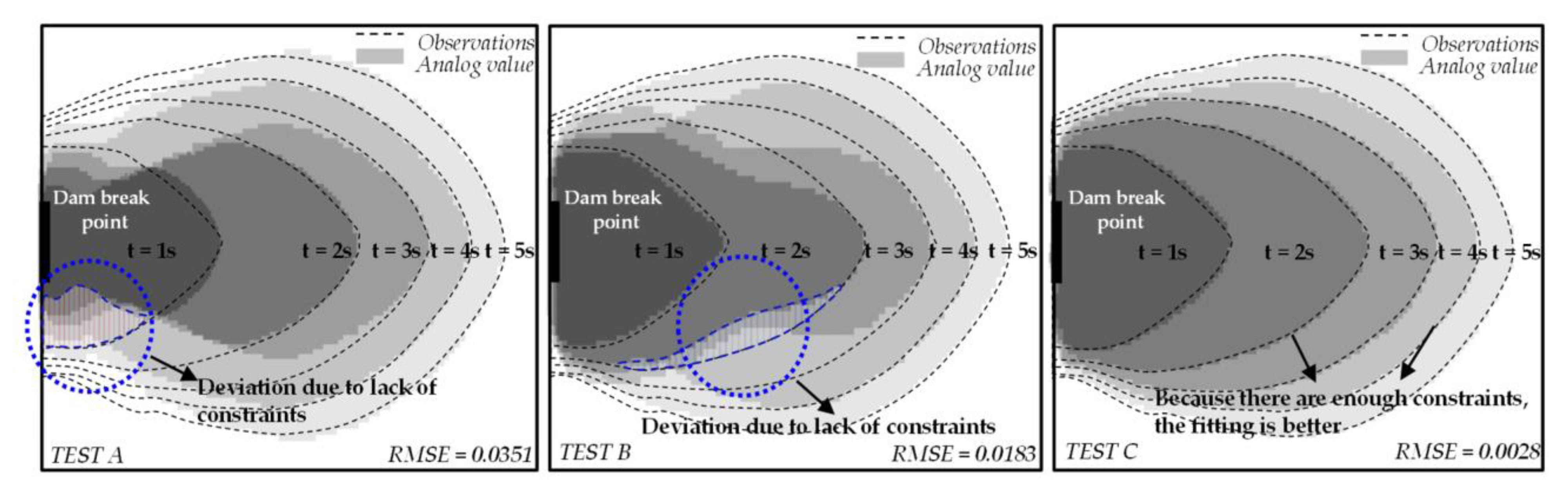
Based on the observation data obtained by the simulation, we carried out the numerical experiments of the model. We recorded the actual submerged range at t = 1, 2, 3, 4, and 5 s. Furthermore, we designed three sets of experimental programs based on the data in the submerged area. The specific experimental programs are shown in

Table 3. Experimental protocol description.

Test Protocol	Test Protocol Description
Test A	Only the submerged range at t = 5 s
Test B	Only the submerged range at t = 1, 5 s
Test C	Only the submerged range at t = 1, 3, 5 s

.

In those cases, we first established an initial continuous function ${\varphi }_0\left(x,y\right)=\sqrt{{\left(x-x_0\right)}^2+{\left(y-y_0\right)}^2}-r$, and the zero isosurface ${\mathrm{C}}_0\left(t\right)=\left\{\left(i,j\right)\in \mathsf{\Omega }:{\varphi }_0\left(x,y\right)=0\right\}$ of the function was the initial evolution shape of the flood inundation range at time 0. Then we used Formula (20) to perform the iterative evolution of the surface function. The intersection of the surface with the plane created the implicit contour of the flood inundation range, as shown in Figure 12.

Figure 13 shows the comparison between the boundary line of the submerged area calculated by using different sets of observation data and the actual value. When only the final state data (Test A) was used as the input parameter, the simulated value differed significantly from the observed data, especially at the moment of t = 1. When the initial state was added to the input parameter (Test B), although the intermediate outcomes at t = 2 and 3 s were still unsatisfactory, the degree of compliance had improved enormously. When the data of the submerged range at t = 1, 3, and 5 s were all used as input parameters (Test C), the simulation effect was close to the actual value. It could be seen that the effect of the simulation was closely related to the constraints in the simulation process. More restrictions could better control the deformation of the curve and make the curve evolve in the right direction. The shorter the time interval, the more constraints and the more accurate the simulation results.

4. Case Study

A real-life environment that requires a solution to the proposed challenge was chosen to further validate our model’s effectiveness.

4.1. Study Site

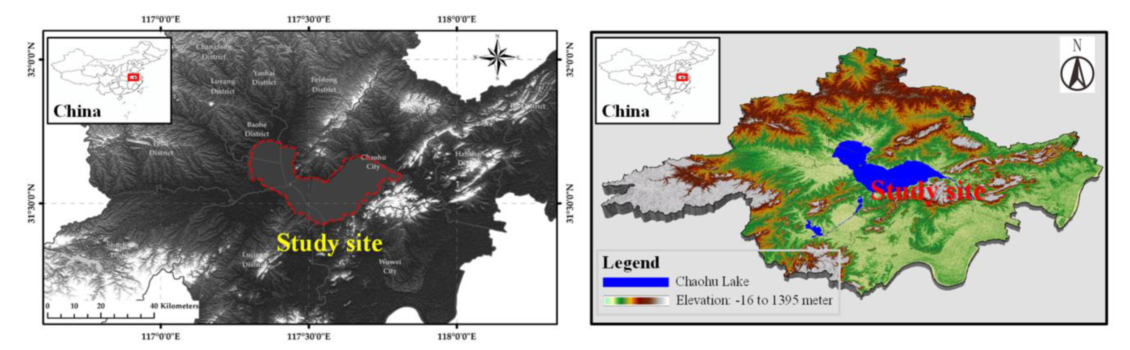
We selected Chaohu Lake and surrounding areas as the study areas, aiming to research the impact of the 2020 flood in the Chaohu Lake basin. The Chaohu Lake Basin, located in the middle of Anhui Province, includes 13 county-level units in Chaohu City, Feidong County, Feixi County, Lujiang County, Changfeng County, Shushan District, Luyang District, Yaohai District, Baohe District, Hanshan County, He County, Wuwei City, and Shucheng County. Its latitude ranges from 30°57′05″ N to 32°32′20″ N, and longitude ranges from 116°25′20″ E to 118°30′00″ E. Moreover, the geographic location is shown in Figure 14.

4.2. Data Collection and Preprocessing

The data sources used in this paper are shown in

Table 4. Data information used in this paper.

Type	Content	Source	Purpose
Open-source dataset	GID	http://captain.whu.edu.cn/GID/	To create datasets
	AID	https://pan.baidu.com/s/1mifOBv6#list/path=%2F
Remote-sensing data	GF-1	http://www.gscloud.cn/search	To create datasets
	Landsat-8 OLI	http://eds.ceode.ac.cn/nuds/freedataquery	To create datasets and obtain flooding data
Basic geographic data	Elevation Map	https://www.databox.store/Home/Index	To assess the loss of flood damage
	Land-use map	https://www.databox.store/Home/Index
	Chinese administrative divisions map	https://www.databox.store/Home/Index
	Population-density map	https://www.worldpop.org/
	Road-distribution map	https://www.openstreetmap.org/
Statistical data	Anhui Province’s statistical yearbook	http://tjj.ah.gov.cn/ssah/qwfbjd/tjnj/index.html	To verify the accuracy of experimental results
	Official Public Releases	http://yjt.ah.gov.cn/public/9377745/145229191.html

. The data sources of the standard datasets for water-body information extraction produced in this paper were two open-source datasets, Gaofen Image Dataset (GID) [36] and Aerial Image Dataset (AID) [37], GF-1 and Landsat-8 OLI, since they are relatively cost-effective remote-sensing image data and highly accessible. The datasets included images with multiple river scales and various representative interferences, such as mountain shadows, clouds occlusion, road interference, different sand content of the river, dry river bed interference, and mosaic changes of images. The data source of the specific datasets was Landsat-8 OLI, which contained four types: plateau area, mountainous area, built-up area, and multi-water area. The source of flood data in the study area was Landsat-8 OLI. Due to the continuous rainy weather during the flood period, the remote-sensing data were insufficient. Thus, we selected only five phases of Landsat-8 OLI remote-sensing images of relatively good quality across the life cycle of the flood event of the Chaohu Lake Basin, and the acquisition time was 17 May, 20 July, 5 August, 6 September, and 24 October in 2020. The geographic data were used to establish the flood loss assessment model in the Chaohu Lake Basin. In addition, official statistics data of Anhui Province and public-releases data were used to verify the correctness of experimental results.

4.3. Results and Discussion

The whole simulation was subdivided into two parts as well. It starts with the extraction of information on the distribution of water bodies at different points in time through remote-sensing imagery. Secondly, we intend to obtain a dynamic continuous flood process by modeling this discrete water level distribution information. Finally, we will conclude with a systematic evaluation and analysis of the probable impacts of this flooding process.

4.3.1. Flood Extraction Results on the Study Site

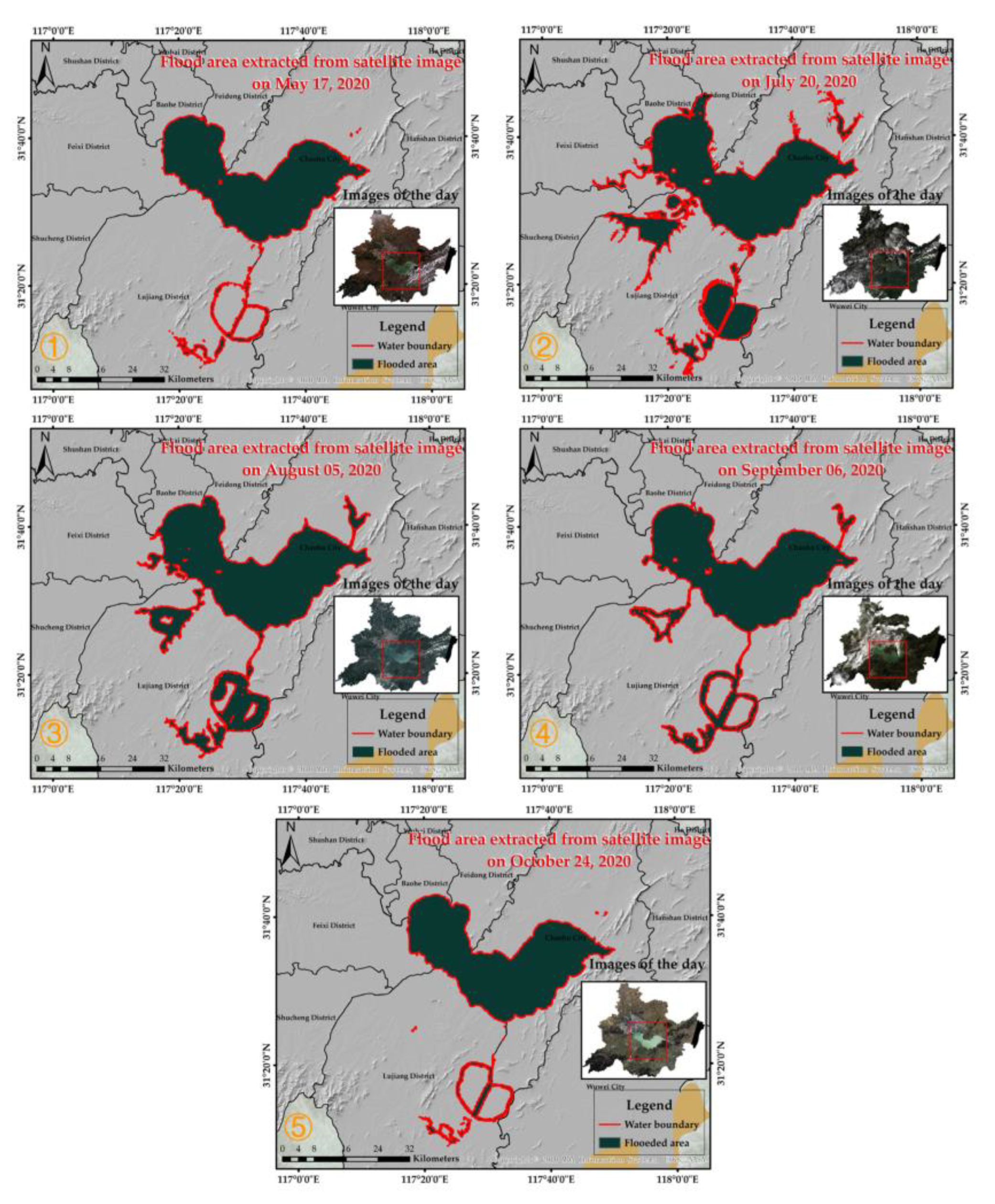
The proposed U-Net model was used to extract the flood, and we could see the comparison of satellite images and extracted areas in Figure 15. The total outcomes of flood extraction based on date-specific remote-sensing images are shown in Figure 16. According to the consequences, we could deduce that the regions affected by the flood in the Chaohu Lake Basin were primarily located in the southwest, followed by the northeast. 20 July was almost the peak time of this flood event, and the areas around Chaohu Lake were more or less submerged. Before 5 August, the floods did not fall significantly. By 6 September, the floods in the northern area had subsided, and only the southwestern areas were still severely affected. On 24 October, the flooding situation was similar to when there was no flood on 17 May. According to the flooding-related information assembled, flood peaks in various regions were concentrated on 18 to 24 July, and the floods had receded before 30 September. It could be seen that there was a good concordance with our extraction results.

Simultaneously, the water-body ranges extracted from the remote-sensing image on 17 May were selected as the original input data as the start time of the flood. The flood inundation range on 20 July was the peak-time data, and the range on 24 October was selected as the input data of the low-tide period. Flood-spreading process simulation was carried out through the water-boundary tracking model. Meanwhile, the extraction results from 5 August and 6 September were used as a validation dataset to verify the accuracy of the simulation.

4.3.2. Overland Flow Routing Simulation Result

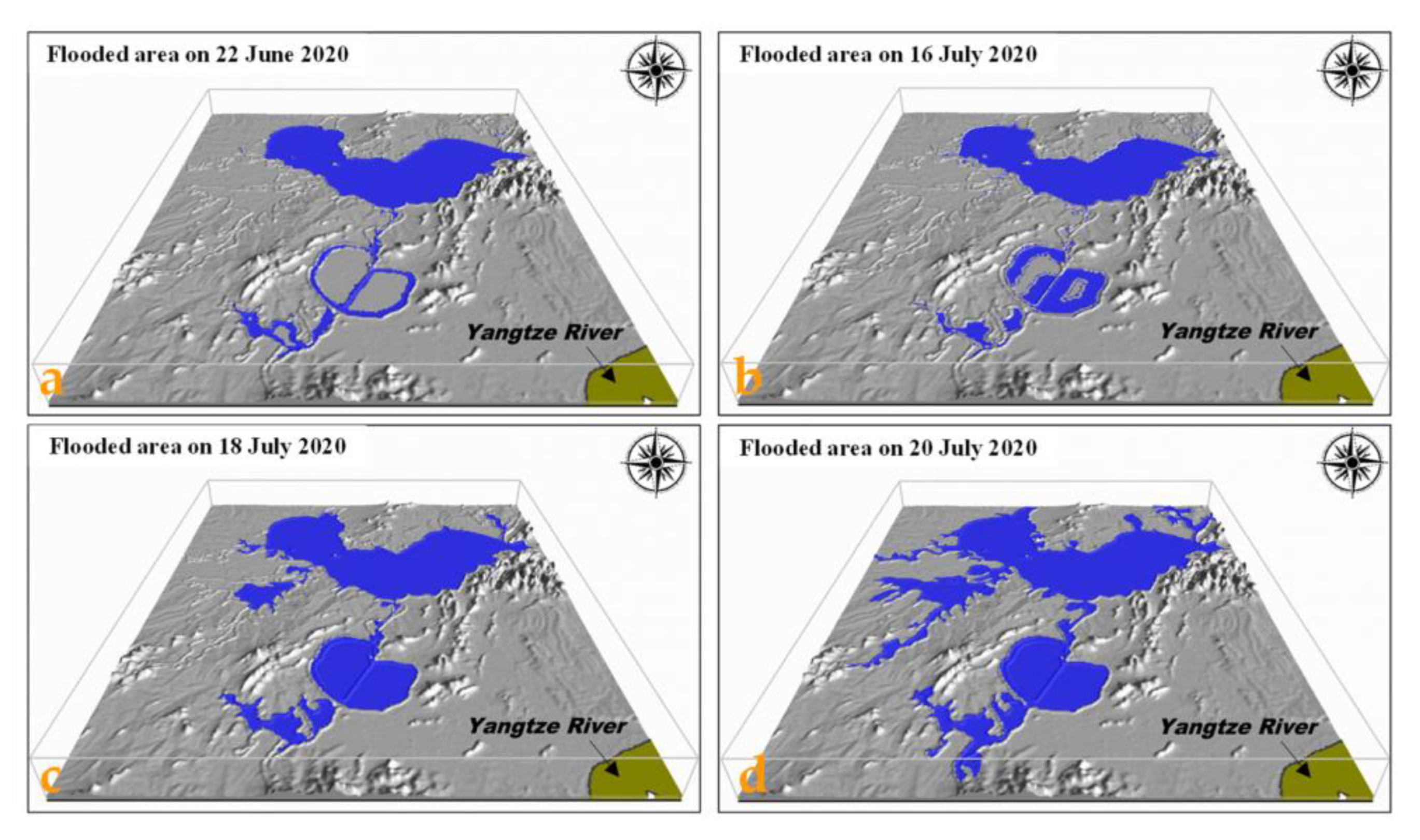
We finally gained the daily flood inundation simulation results from 15 June to 30 September through the active boundary tracking model. Considering the different characteristics of the floodwater increase and decrease, the simulation process was divided into two stages: the rising water and falling water stage. The results are shown in Figure 17 and Figure 18, respectively.

I Simulation of water rising process

Figure 17 shows that the inundation area of the Chaohu Lake Basin did not increase significantly until 22 June. The spread of flooding became apparent on 16 July, and a sizeable flooded area appeared in the southwest. On 18 July, the low-lying areas around Chaohu Lake were flooded rapidly. The southwestern regions saw the fastest water rise, followed by the northeast areas, and the southeast areas had the lightest water accumulation. The flooding situation in Lujiang County and Chaohu City was even more serious. On 20 July, the flooded area reached its maximum.

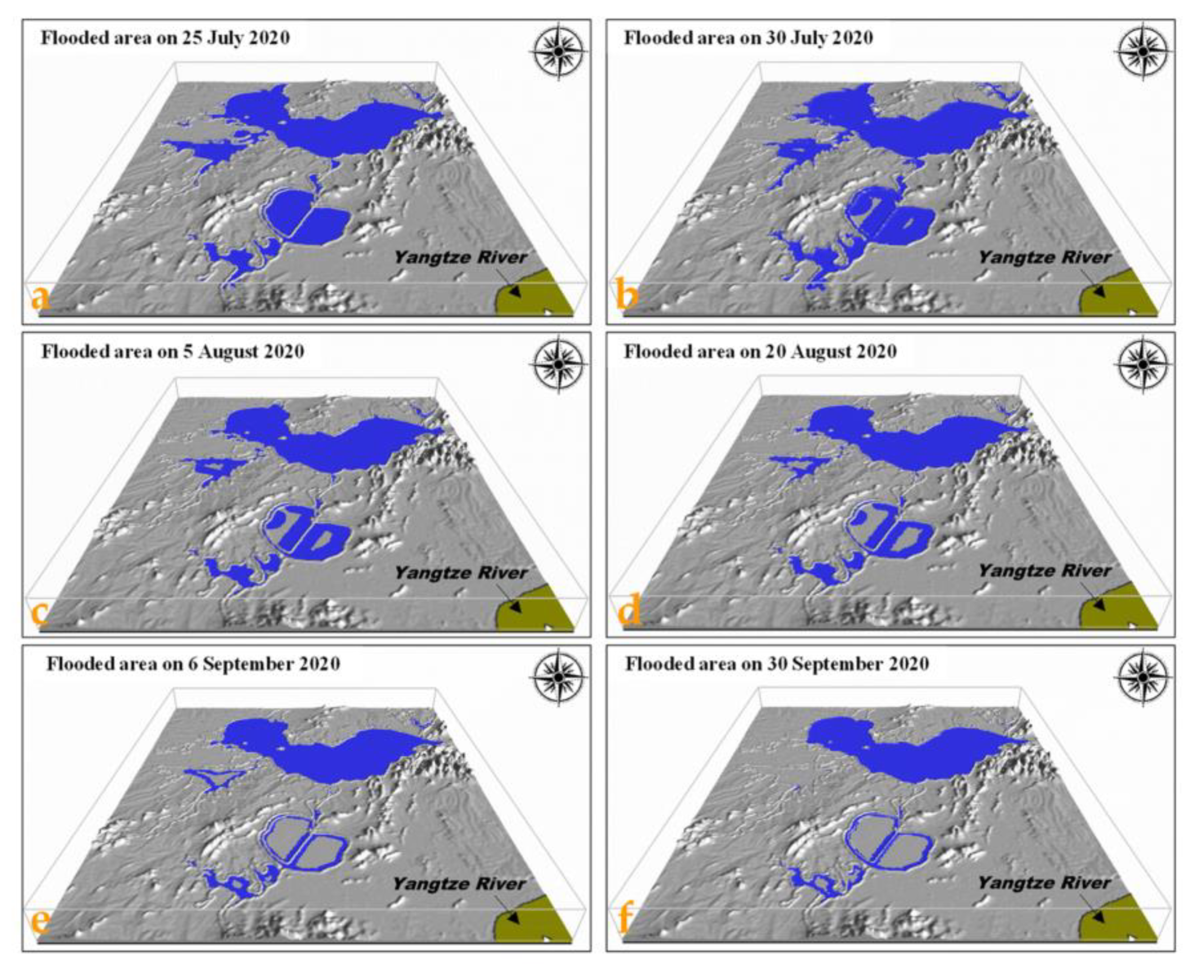
II Simulation of water-receding process

Figure 18 shows that after the flood’s peak on 20 July, the flood area began to decrease. The floods in the northwest and southeast areas receded promptly, while the southwest areas receded gradually. On 20 August, the northwestern regions dried up, and on 25 August, the northeastern part also retreated. Moreover, Lujiang County continued to be flooded until the end of September.

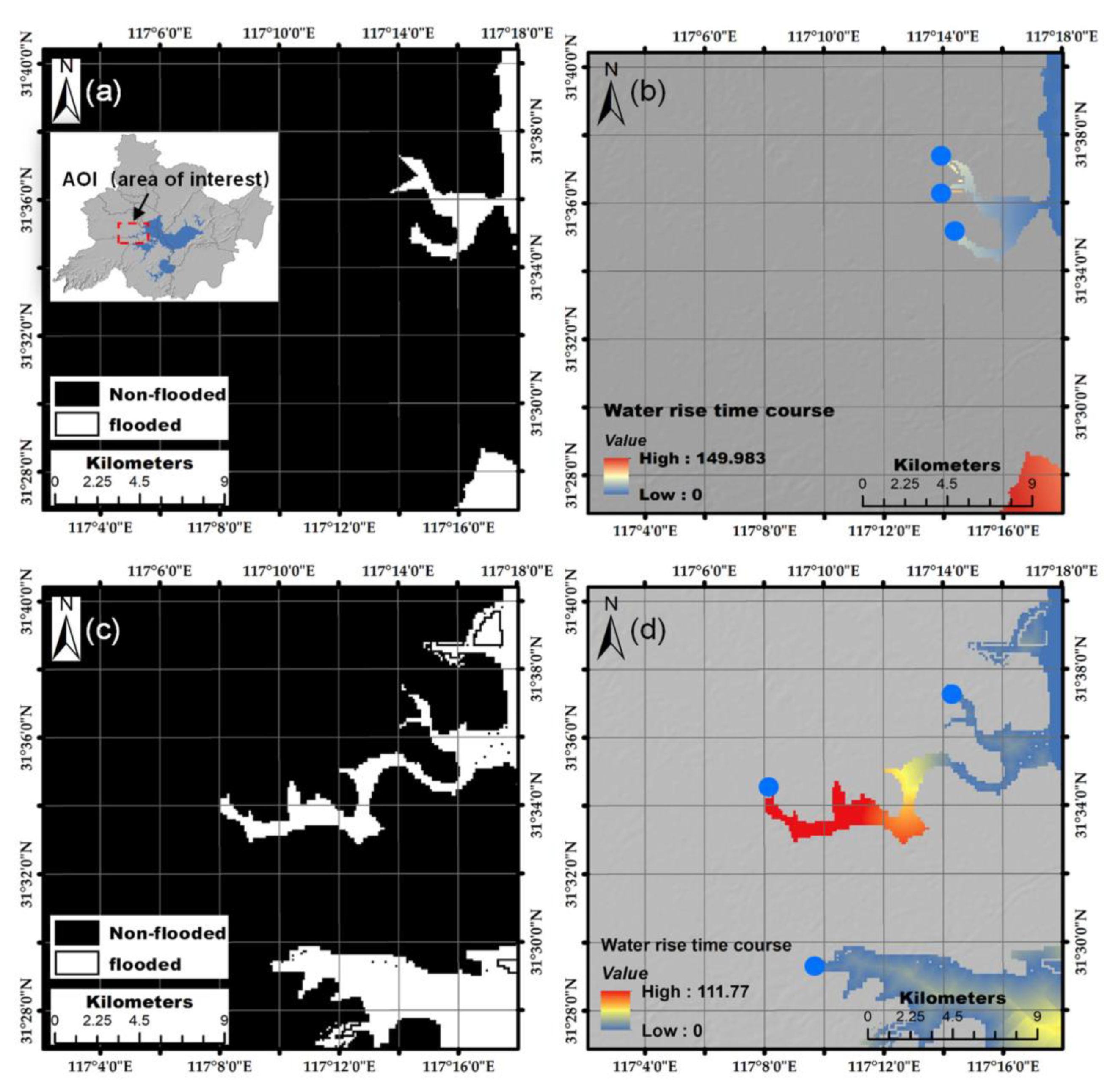
To demonstrate the effectiveness of the model simulated in detail, we chose a tiny region on the western side of the study area as an area of interest (AOI). Here we displayed results in terms of binary maps of flood extents over the selected AOI shown in panel (a), together with an example of a water rise course map in panel (b) as provided for the same day in Figure 19. More details of the spatial inundation pattern were visible in the selected region. The result showed that the tracking model based on remote-sensing observation data could swiftly generate a higher resolution and accurate flood disaster map. The evolution process could be seen more intuitively.

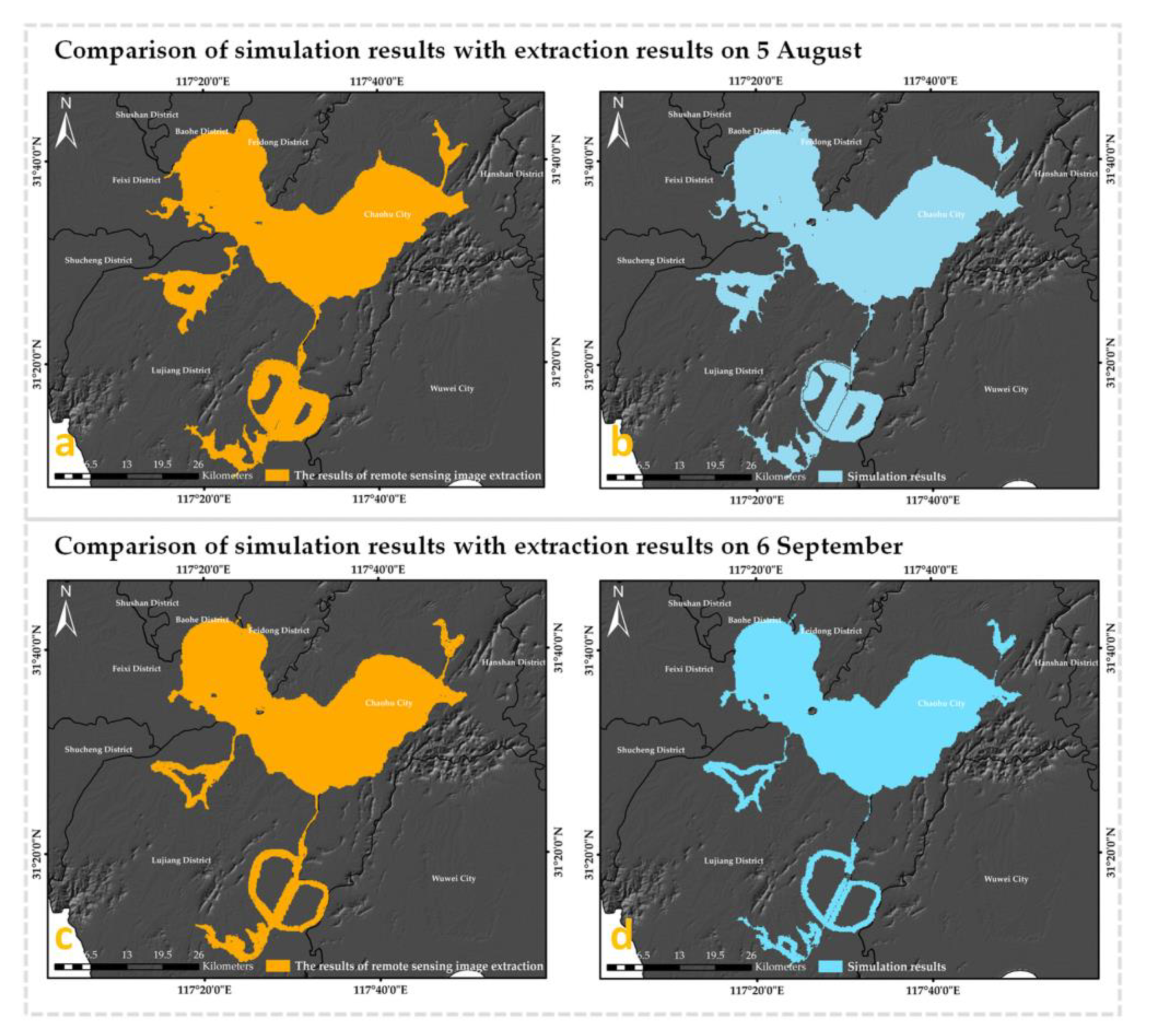
To verify the accuracy of this method, we established a confusion matrix for accuracy evaluation by comparing the simulation results on 5 August and 6 September with the remote-sensing image extraction results, as shown in Figure 20. The results are shown in

Table 5. Accuracy verification between simulation and extraction results.

Data Simulation Time	Correct Rate	Misclassification Rate	Omission Rate	Kappa
August 5	0.9540	0.0602	0.0272	0.9078
September 6	0.9606	0.0470	0.0288	0.9211

. The Kappa values of the two tests were 0.9078 and 0.9211, which showed that the simulation results and the remote-sensing image extraction results were in good agreement.

In addition, we picked certain videos, reports, and bulletins released by authoritative agencies to provide supplementary validation, as shown in

Table 6. The list of information released by authoritative agencies providing complementary validation.

Time	Place	Description of Event	Results Involved	Data Source
19 August 2020	Feidong County	There was flood water depth over 3 meters in some parts, on 7 August, and on 17 August, it was receded [38].	7.30 8.5 8.30	Anhui Broadcasting Corporation
22 September 2020	Feixi County	Floodwaters have primarily receded in mid-September [39].	9.6 9.30	Anhui Broadcasting Corporation
29 September 2020	Lujiang County	There was still no receding flooding in Tongda town [40].	9.30	Lujiang County Government Official Website
20 October 2020	Lujiang County	Flood in Baihu Farm was drained at the end of September [41].	9.30	Anhui Provincial Bureau of Statistics

. The simulation outcomes better match the actual situation described in the validation information.

4.3.3. Prediction of Potential Flooding Risk

To offer decision support to policymakers, we needed to estimate flood risk adequately. Thus, seven indicators were selected from the characteristics of the study area and flood inundation attributes to form a flood-disaster loss-evaluation system. These seven indicators are shown in

Table 7. Indicator system for flood-risk assessment.

Category	Evaluation Indicator	Serial Number
Study area characteristics	The census block density	U1
	Road network density	U2
	Building density	U3
	Farmland density	U4
Flood inundation attributes	Maximum submerged area	U5
	Average maximum submerged depth	U6
	Average submerged duration	U7

. The indicators U1, U2, U3, and U4 were from the basic geographic data on the Internet. The maximum submerged area indicator came from the extraction results of remote-sensing images. The average maximum submerged depth indicator was obtained by kriging interpolation based on the elevation points of the submerged boundary in ArcGIS [42]. The average flooding duration indicator was obtained by creating random sample points on the continuous simulation results and calculating the time difference between the beginning and the end of the flooding.

We divided the degree of flooding loss into five grades and separated the interval of each indicator. The parameters $E_x$ and $E_n$ of the cloud model were calculated by $E_{x ij}=\frac{x_{ij}^1+x_{ij}^2}{2}$ and $E_{n ij}=\frac{x_{ij}^2-x_{ij}^1}{2.355}$, and the value of the parameter $H_e$ was manually adjusted through multiple trials. In these formulas, $x_{ij}^1 \mathrm{and} x_{ij}^2$represented the lower and upper boundary values of a specific interval of an indicator, respectively. The calculated parameter matrix of the cloud model is shown in

Table 8. Parameter matrix for the risk-assessment cloud model.

Evaluation Index	Very Low Loss	Low Loss	Moderate Loss	High Loss	Very High Loss
U1	(215.76, 183.24, 0.1)	(531.99, 85.21, 0.1)	(1148.13, 437.95, 0.1)	(2032.10, 312.76, 0.1)	(3143.35, 630.97, 0.1)
U2	(0.0588, 0.0499, 0.01)	(0.1791, 0.0523, 0.01)	(0.3318, 0.0773, 0.01)	(0.6705, 0.2103, 0.01)	(1.0329, 0.0975, 0.01)
U3	(0.0240, 0.0203, 0.01)	(0.0970, 0.0417, 0.01)	(0.1951, 0.0417, 0.01)	(0.2932, 0.0417, 0.01)	(0.3913, 0.0417, 0.01)
U4	(0.1288, 0.1093, 0.01)	(0.3293, 0.0610, 0.01)	(0.4967, 0.0811, 0.01)	(0.6374, 0.0383, 0.01)	(0.7249, 0.0360, 0.01)
U5	(0.50, 0.42, 0.01)	(1.50, 0.42, 0.01)	(2.57, 0.48, 0.01)	(4.12, 0.84, 0.01)	(6.00, 0.76, 0.01)
U6	(1.75, 1.49, 0.1)	(7.01, 2.98, 0.1)	(22.06, 9.80, 0.1)	(57.04, 19.90, 0.1)	(127.60, 40.03, 0.1)
U7	(0.61, 0.52, 0.1)	(2.12, 0.76, 0.1)	(5.46, 2.07, 0.1)	(9.78, 1.61, 0.1)	(15.76, 3.47, 0.1)

.

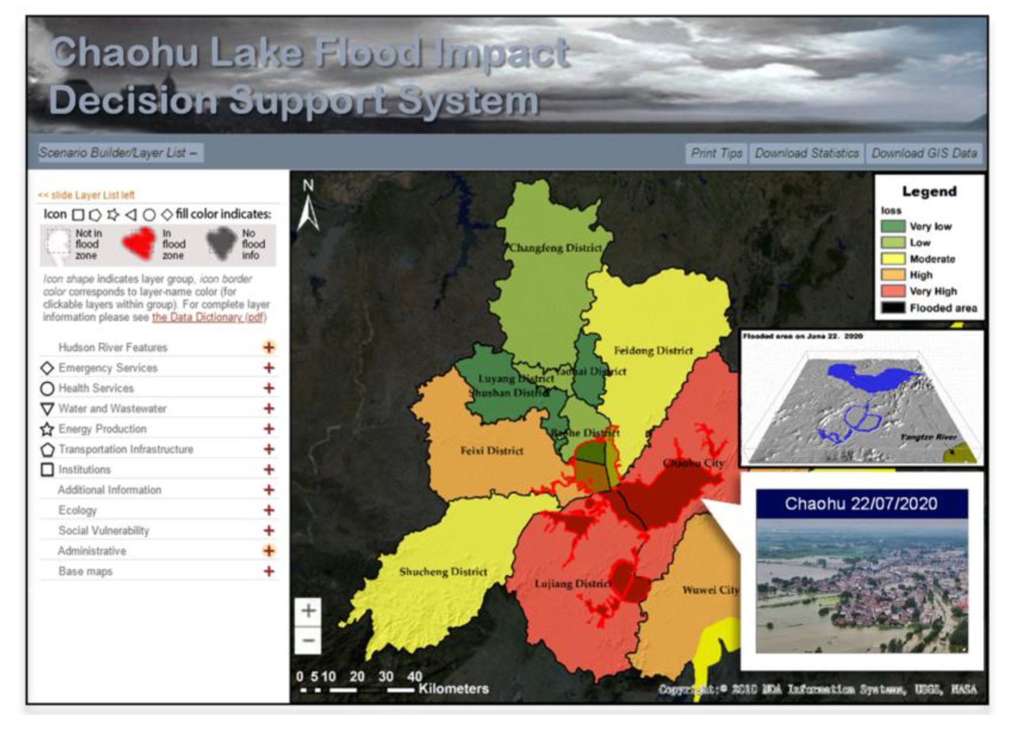
For each indicator, according to the cloud model parameter matrix shown in

Table 9. The results of the Chaohu Basin Flood Hazard Risk Assessment.

County Unit	Very Low Loss	Low Loss	Moderate Loss	High Loss	Very High Loss	Level	Official Released
Yaohai District	0.517	0.223	0.102	0.054	0.019	Very low loss	No mention
Luyang District	0.172	0.629	0.264	0.032	0.057	Low loss	No mention
Shushan District	0.463	0.209	0.083	0.097	0.000	Very low loss	No mention
Baohe District	0.231	0.629	0.264	0.032	0.057	Low loss	No mention
Chaohu City	0.000	0.038	0.221	0.375	0.426	Very high loss	Hard-hit
Changfeng County	0.379	0.425	0.154	0.169	0.022	Low loss	No mention
Feidong County	0.125	0.301	0.395	0.113	0.025	Moderate loss	No mention
Feixi County	0.104	0.092	0.368	0.394	0.212	High loss	Hard-hit
Lujiang County	0.000	0.152	0.104	0.328	0.539	Very high loss	Hard-hit
Wuwei County	0.043	0.116	0.253	0.314	0.182	High loss	Hard-hit
Shucheng County	0.079	0.211	0.535	0.268	0.118	Moderate loss	Hard-hit
Hanshan County	0.108	0.102	0.294	0.377	0.176	High loss	Hard-hit
He County	0.215	0.208	0.317	0.142	0.093	Moderate loss	Hard-hit

, we could generate the certainty degree matrix under different loss levels through the forward cloud generator. Considering the randomness of the calculation results, we calculated 1000 times to obtain higher accuracy. After obtaining the certainty degree matrixes of all indicators, combined with the weight coefficient calculated through the entropy weight method, the comprehensive flooding loss evaluation of 13 county-level regions in the Chaohu Lake Basin could be performed. The results of flooding loss evaluation are shown in Table 9, and the distribution of disaster losses and the two-dimensional flood impact assessment visualization platform is shown in Figure 21. Lujiang County and Chaohu City, which were the closest to Chaohu Lake, were the worst affected. Meanwhile, Yaohai District and Shushan District, which were far away, were the least affected. The more severe loss areas were primarily distributed in the southwest and northeast. According to the Emergency Management Department of Anhui Province, Lujiang County, Feixi County, Chaohu City, Shucheng County, Hanshan County, He County, and Wuwei County in the Chaohu Lake Basin were considered as the hard-hit counties, and the statistics were in good agreement with our evaluation results (http://yjt.ah.gov.cn/public/9377745/145229191.html, accessed on 20 October 2020).

5. Conclusions

Rapid-response mapping of floodwater extents in flood events, such as “coastal flood” and “fluvial flood”, while essential for early damage assessment and rescue operations, also presents significant image interpretation challenges. Images from the visible band (red–green–blue (RGB)) remote sensors are the most common and cost-effective for real-time applications. Despite the poor quality of optical remote-sensing images caused by the weather conditions experienced during the flood event, this study developed a robust decision support system based on limited and intermittent optical remote-sensing data to fully and effectively use the optical remote-sensing data. The system was constructed based on two primary modules. An automatized multi-scale water extraction model was established to extract visible floodwater, using RGB band digital numbers. Visible floodwater denotes the floodwater on the ground surface that can be observed by remote sensing and is a crucial information source for the analysis of real-time floodwater extent; floodwater under tree canopies and in shadows was excluded from the visible floodwater class. The methodology was applied to delineate visible floodwater distribution from selected Landsat-8 optical image data acquired during the 2020 Chaohu flood event. The spatial resolution of the identified outcomes was high, but the temporal resolution was low. In addition, we developed a waterfront active tracking model to simulate the dynamic and continuous flood-range change based on the obtained flood extraction results, converting the flooding process into the numerical solution of the partial differential equation of the boundary function, and ultimately received a flooding process with a high resolution in both time and space.

An essential conclusion is that relatively high-resolution optical RGB imagery can provide the source of information for rapid response mapping of visible floodwater distributions during the life cycle of a flood event, despite the limited lower temporal resolution. The decision support system developed in this study could be used as a primary tool for rapid extraction of the visible floodwater from RGB image data and estimate flood risk through temporal interpolation. The application results showed that this system had high computational efficiency and noticeable visualization effects, providing a quick overview of the condition and comprehensive insights into the affected area for decision-makers and relief organizations to distribute their resources with maximum efficiency.

In future work, we expect to compare and consider selecting multi-source satellite data with relatively higher spatial and temporal resolution and use data-fusion techniques to further improve the accuracy and real-time performance of the system.

References

- Shao, M.; Gong, Z.; Xu, X. Risk assessment of rainstorm and flood disasters in China between 2004 and 2009 based on gray fixed weight cluster analysis. Nat. Hazards. 2014, 71, 1025–1052. [Google Scholar] [CrossRef]
- Nobre, G.G.E.; Jongman, B.; Aerts, J.; Ward, P.J. The role of climate variability in extreme floods in Europe. Environ. Res. Lett. 2017, 12, 84012. [Google Scholar] [CrossRef]
- Schumann, G.; Baldassarre, G.D.; Bates, P.D. The Utility of Spaceborne Radar to Render Flood Inundation Maps Based on Multialgorithm Ensembles. IEEE Trans. Geosci. Remote Sens. 2009, 47, 2801–2807. [Google Scholar] [CrossRef]
- Zhang, Y.; Crawford, P. Automated Extraction of Visible Floodwater in Dense Urban Areas from RGB Aerial Photos. Remote Sens. Basel. 2020, 12, 2198. [Google Scholar] [CrossRef]
- Hong, S.; Jang, H.; Kim, N.; Sohn, H.G. Water Area Extraction Using RADARSAT SAR Imagery Combined with Landsat Imagery and Terrain Information. Sensors 2015, 15, 6652–6657. [Google Scholar] [CrossRef]
- Zhang, J.; Wang, X.Y.; Gao, C.; Ren, X.; Xie, J. Research on the Method of Extracting Water Information in Dongping Lake by Using Landsat TM Image. Geomat. Spat. Inf. Technol. 2012, 35, 23–27. [Google Scholar]
- McFEETERS, S.K. The use of the Normalized Difference Water Index (NDWI) in the delineation of open water features. Int. J. Remote Sens. 1996, 17, 1425–1432. [Google Scholar] [CrossRef]
- Scott, W.C.; Owen, K.; Miles, E.S.; Quincey, D.J. Optimising NDWI supraglacial pond classification on Himalayan debris-covered glaciers. Remote Sens. Environ. 2018, 217, 414–425. [Google Scholar]
- Kelly, J.T.; Gontz, A.M. Using GPS-surveyed intertidal zones to determine the validity of shorelines automatically mapped by Landsat water indices. Int. J. Appl. Earth Obs. 2018, 65, 92–104. [Google Scholar] [CrossRef]
- Worden, J.; Beurs, K.M.D. Surface water detection in the Caucasus. Int. J. Appl. Earth Obs. 2020, 91, 102159. [Google Scholar] [CrossRef]
- Acharya, T.D.; Lee, D.H.; Yang, I.T.; Lee, J.K. Identification of Water Bodies in a Landsat 8 OLI Image Using a J48 Decision Tree. Sensors 2016, 16, 1075. [Google Scholar] [CrossRef] [PubMed] [Green Version]
- Fu, J.; Wang, J.; Li, J. Study on the Automatic Extraction of Water Body from TM Image Using Decision Tree Algorithm. Available online: https://ui.adsabs.harvard.edu/abs/2008SPIE.6625E..02F/abstract (accessed on 9 September 2007).
- Yong, H.D.; Jing, L.I.; Chen, Y.H.; Jiang, W.G. Water and Settlement Area Extraction from Single-band, Single-polarization SAR Images Based on SVM Method. J. Image Graph. 2008, 13, 257–263. [Google Scholar]
- Sarp, G.; Ozcelik, M. Water body extraction and change detection using time series: A case study of Lake Burdur, Turkey. J. Taibah Univ. Sci. 2016, 11, 381–391. [Google Scholar] [CrossRef] [Green Version]
- Byoung, K.; Hyeong, K.; Jae, N. Classification of Potential Water Bodies Using Landsat 8 OLI and a Combination of Two Boosted Random Forest Classifiers. Sensors 2015, 15, 13763–13777. [Google Scholar]
- Paul, A.; Tripathi, D.; Dutta, D. Application and comparison of advanced supervised classifiers in extraction of water bodies from remote sensing images. Sustain. Water Resour. Manag. 2018, 4, 905–919. [Google Scholar] [CrossRef]
- Guo, H.; He, G.; Jiang, W.; Yin, R.; Leng, W. A Multi-Scale Water Extraction Convolutional Neural Network (MWEN) Method for GaoFen-1 Remote Sensing Images. Int. J. Geo-Inf. 2020, 9, 189. [Google Scholar] [CrossRef] [Green Version]
- Wu, Z.; Gao, Y.; Li, L.; Xue, J.; Li, Y. Semantic segmentation of high-resolution remote sensing images using fully convolutional network with adaptive threshold. Connect. Sci. 2019, 31, 169–184. [Google Scholar] [CrossRef]
- Feng, W.; Sui, H.; Huang, W.; Xu, C.; An, K. Water Body Extraction From Very High-Resolution Remote Sensing Imagery Using Deep U-Net and a Superpixel-Based Conditional Random Field Model. IEEE Geosci. Remote S 2018, 1–5. [Google Scholar] [CrossRef]
- Yang, Z.; Wen-Hao, O.U.; Liu, X.Y.; Chuang, L.I.; Fei, X.Z.; Zhao, B.B.; Liu, L.; Xiao, M.A. Water information extraction for high resolution remote sensing image based on LinkNet convolutional neural network. J. Yunnan Univ. Nat. Sci. Ed. 2019, 41, 932–938. [Google Scholar]
- Li, Z.; Wang, R.; Zhang, W.; Hu, F.; Meng, L. Multiscale Features Supported DeepLabV3+ Optimization Scheme for Accurate Water Semantic Segmentation. IEEE Access. 2019, 7, 1. [Google Scholar] [CrossRef]
- Ronneberger, O.; Fischer, P.; Brox, T. U-Net: Convolutional Networks for Biomedical Image Segmentation; Navab, N., Hornegger, J., Wells, W.M., Frangi, A.F., Eds.; Springer International Publishing: Cham, Switzerland, 2015; pp. 234–241. [Google Scholar]
- Liang, Q.; Du, G.; Hall, J.W.; Borthwick, A.G. Flood Inundation Modeling with an Adaptive Quadtree Grid Shallow Water Equation Solver. J. Hydraul. Eng. 2015, 134, 1603–1610. [Google Scholar] [CrossRef]
- Teng, J.; Jakeman, A.J.; Vaze, J.; Croke, B.; Dutta, D.; Kim, S. Flood inundation modelling: A review of methods, recent advances and uncertainty analysis. Environ. Modell. Softw. 2017, 90, 201–216. [Google Scholar] [CrossRef]
- Mason, D.C.; Bates, P.D.; Amico, J. Calibration of uncertain flood inundation models using remotely sensed water levels. J. Hydrol. 2009, 368, 224–236. [Google Scholar] [CrossRef]
- Lai, X.J.; Jiang, J.H.; Huang, Q.; Wu, D. A Level-set Based Varistional Method for Data Assimilation of Flood Extend into a Two-dimensional Flood Model. J. Basic Sci. Eng. 2013, 5, 1018–1026. [Google Scholar]
- Zhang, L.C.; Li, G.Q.; Yu, W.Y.; Ran, Q. Approach to simulating the spatial-temporal process of flood inundation area. Remote Sens. Land Resour. 2017, 29, 92–96. [Google Scholar]
- Shamsolmoali, P.; Zareapoor, M.; Wang, R.; Zhou, H.; Yang, J. A Novel Deep Structure U-Net for Sea-Land Segmentation in Remote Sensing Images. IEEE J. Stars. 2019, PP, 1–14. [Google Scholar] [CrossRef] [Green Version]
- Li, S.; Deng, M.; Lee, J.; Sinha, A.; Barbastathis, G. Imaging through glass diffusers using densely connected convolutional networks. Optica 2017, 5, 7. [Google Scholar] [CrossRef]
- Tao, Y.; Xu, M.; Lu, Z.; Zhong, Y. DenseNet-Based Depth-Width Double Reinforced Deep Learning Neural Network for High-Resolution Remote Sensing Image Per-Pixel Classification. Remote Sens. Basel. 2018, 10, 779. [Google Scholar] [CrossRef] [Green Version]
- Wang, Z.; Gao, X.; Zhang, Y.; Zhao, G. MSLWENet: A Novel Deep Learning Network for Lake Water Body Extraction of Google Remote Sensing Images. Remote Sens. Basel. 2020, 12, 4140. [Google Scholar] [CrossRef]
- Sun, H.; Wang, J.; Ye, W. A Data Augmentation-Based Evaluation System for Regional Direct Economic Losses of Storm Surge Disasters. Int. J. Env. Res. Pub. He. 2021, 18, 2918. [Google Scholar] [CrossRef]
- Zheng, Y.; Sun, H. An Integrated Approach for the Simulation Modeling and Risk Assessment of Coastal Flooding. Water 2020, 12, 2076. [Google Scholar] [CrossRef]
- Li, D.Y.; Meng, H.J.; Shi, X.M. Membership Clouds and Membership Cloud Generators. Comput. R D 1995, 32, 15–20. [Google Scholar]
- Ji, Y.; Huang, G.H.; Sun, W. Risk assessment of hydropower stations through an integrated fuzzy entropy-weight multiple criteria decision making method: A case study of the Xiangxi River. Expert Syst. Appl. 2015, 42, 5380–5389. [Google Scholar] [CrossRef]
- Tong, X.Y.; Xia, G.S.; Lu, Q.; Shen, H.; Zhang, L. Land-Cover Classification with High-Resolution Remote Sensing Images Using Transferable Deep Models. arXiv 2019, arXiv:1807.05713. [Google Scholar] [CrossRef] [Green Version]
- Xia, G.S.; Hu, J.; Hu, F.; Shi, B.; Zhang, L. AID: A Benchmark Data Set for Performance Evaluation of Aerial Scene Classification. IEEE T. Geosci. Remote. 2017, 55, 3965–3981. [Google Scholar] [CrossRef] [Green Version]
- Anhui Broadcasting Corporation. Available online: http://www.ahtv.cn/pindao/ahjs/dysj/split/2020/0819/001436190.html (accessed on 19 August 2020).
- Anhui Broadcasting Corporation. Available online: http://www.ahtv.cn/pindao/ahgg/yx60/split/2020/0921/001446560.html (accessed on 22 September 2020).
- Lujiang County Government Official Website. Available online: http://www.lj.gov.cn/zwdt/xzdt/119897595.html (accessed on 29 September 2020).
- Anhui Provincial Bureau of Statistics. Available online: http://tjj.ah.gov.cn/public/6981/145230531.html (accessed on 20 October 2020).
- Shen, Q.; Gao, W.; Li, X.; Zhou, Y.T.; Zhou, Y.H. Monitoring of Flood Depth in Small and Medium-sized Basins Using GF-1 WFV Images. Remote Sens. Inf. 2019, 34, 87–92. [Google Scholar]
Figure 1.
Severe floods in Southern China in 2020. The increasing water level has caused many low-lying districts to be flooded (a), leading to severe damage (b).
Figure 2.
Flowchart of this study.
Figure 3.
The search space of the Dense Connection Block.
Figure 4.
Dataset-generation process. After data preparation (a), processing (b), and post-processing (c), common and specific datasets (d) are obtained.
Figure 5.
Some samples in the specific datasets: (a–c) belong to built-up areas; (d–f) belong to mountainous areas; (g–i) belong to plateau areas; (j–l) belong to multi-water areas.
Figure 6.
Front of the flood inundation range propagating with speed, .
Figure 7.
Consider all possible cases in the position of the curve. The fitting term is minimized only when the curve is on the object’s boundary.
Figure 8.
The overall framework and composition of the system.
Figure 9.
Comparison of water extraction results made by different models: (a–d), respectively, correspond to samples taken from plateau area, built-up area, mountainous areas, and multi-water areas.
Figure 10.
Dike breach experiment: (a) presents the rupture flow process, and the red curve represents the change of unit discharge over time; (b) presents the flow of water over ground of different roughness, with the blue curve representing the current water boundary.
Figure 11.
Simulation process based on a 2D hydrodynamic model: (a–f) respectively correspond to the simulation state of water flow at t = 0–5 s.
Figure 12.
The implicit contour of the flood inundation extent. The evolution of the profile of the flood inundation extent at t = 0–5 s is shown along the direction of the arrow.
Figure 13.
Comparison of the simulation performance of flooding processes in the case of dam breach with different initial conditions. From left to right, the outcomes of Test A, Test B, and Test C are respectively represented. The time unit in the graphs is second.
Figure 14.
The geographic location of the study area and its terrain map.
Figure 15.
Comparison of satellite image and extracted areas. The two illustrative regions are located in the northwestern and northeastern parts of the study area. The left portion represents the original remote-sensing satellite image, and the right portion represents the extraction results of the water bodies.
Figure 16.
The extraction results of the flood event, using the proposed model. The five images correspond to the extraction outcomes on 17 May, 20 July, 5 August, 6 September, and 24 October, in 2020.
Figure 17.
Simulation of flood rising process: (a–d), respectively, correspond to the simulation results on 22 June, 16 July, 18 July, and 20 July, in 2020.
Figure 18.
Simulation of flood receding process: (a–f), respectively, correspond to the simulation results on 25 July, 30 July, 5 August, 20 August, 6 September, and 30 September, in 2020.
Figure 19.
Example of flood binary map (a), and corresponding water-rise time course map for the first AOI selected (b). Meanwhile, (c,d) represent the flood binary map and water-rise time course map of the second AOI area respectively.
Figure 20.
Comparison of simulation results with extraction results on 5 August and 6 September: (a,b) represent a comparison on 5 August; (c,d) represent a comparison on 6 September.
Figure 21.
A two-dimensional visualization platform for flood-risk assessment in the Chaohu Lake Basin.