Irrigation Amounts and Timing Retrieval through Data Assimilation of Surface Soil Moisture into the FAO-56 Approach in the South Mediterranean Region

Abstract

Agricultural water use represents more than 70% of the world’s freshwater through irrigation water inputs that are poorly known at the field scale. Irrigation monitoring is thus an important issue for optimizing water use in particular with regards to the water scarcity that the semi-arid regions are already facing. In this context, the aim of this study is to develop and evaluate a new approach to predict seasonal to daily irrigation timing and amounts at the field scale. The method is based on surface soil moisture (SSM) data assimilated into a simple land surface (FAO-56) model through a particle filter technique based on an ensemble of irrigation scenarios. The approach is implemented in three steps. First, synthetic experiments are designed to assess the impact of the frequency of observation, the errors on SSM and the a priori constraints on the irrigation scenarios for different irrigation techniques (flooding and drip). In a second step, the method is evaluated using in situ SSM measurements with different revisit times (3, 6 and 12 days) to mimic the available SSM product derived from remote sensing observation. Finally, SSM estimates from Sentinel-1 are used. Data are collected on different wheat fields grown in Morocco, for both flood and drip irrigation techniques in addition to rainfed fields used for an indirect evaluation of the method performance. Using in situ data, accurate results are obtained. With an observation every 6 days to mimic the Sentinel-1 revisit time, the seasonal amounts are retrieved with R > 0.98, RMSE < 32 mm and bias < 2.5 mm. Likewise, a good agreement is observed at the daily scale for flood irrigation as more than 70% of the detected irrigation events have a time difference from actual irrigation events shorter than 4 days. Over the drip irrigated fields, the statistical metrics are R = 0.74, RMSE = 24.8 mm and bias = 2.3 mm for irrigation amounts cumulated over 15 days. When using SSM products derived from Sentinel-1 data, the statistical metrics on 15-day cumulated amounts slightly dropped to R = 0.64, RMSE = 28.7 mm and bias = 1.9 mm. The metrics on the seasonal amount retrievals are close to assimilating in situ observations with R = 0.99, RMSE = 33.5 mm and bias = −18.8 mm. Finally, among four rainfed seasons, only one false event was detected. This study opens perspectives for the regional retrieval of irrigation amounts and timing at the field scale and for mapping irrigated/non irrigated areas.

1. Introduction

Agriculture is the main consumer of water with about 70–75% of the world’s global freshwater [1,2,3] dedicated to irrigation. Irrigated lands almost doubled over the last five decades [1,4] to cover about 20% of the usable agricultural area increasing the water resources depletion especially in areas already facing water scarcity [5,6]. The latest is unfortunately expected to worsen in the future due to the combined effect of climate change, population growth and agricultural intensification [7]. In the semi-arid Mediterranean region, water consumption through irrigation rises up to 80–90% with an efficiency lower than 50% in several countries. An action on agricultural water demand thus represents the main lever for saving water in the region [8].

Within this context, an accurate knowledge of irrigation water amounts and timing is a prerequisite for improving the efficiency of water use by agriculture at the scales of the decision making: (1) the plot for the farmer who plans its irrigations on a day-to-day basis, (2) the watershed for the basin authorities who distribute water to the different sectors at the seasonal scale and plan the development of the basin and (3) the national territory for the state which defines public policies. The water amounts attributed to the agricultural sector are quite well known at the seasonal scale for the whole watershed by the basin authorities and on a monthly basis for each irrigation districts by the agricultural offices. Yet, irrigation amount and timing are poorly known at the field scale because it is usually not metered neither by the farmers nor by the agricultural office that at best, can provide these information at the farm scale on a monthly basis [8,9]. Nevertheless, some in situ observation exists. Some relies on the relationship between power demand and pumping rate of pumping stations [10] while others rely on statistical surveys but these latter data are associated to several error sources mainly a self-reporting bias and a low spatial accuracy and temporal resolution [11,12]. By contrast, the increasing availability of remote sensing observations with high spatial and temporal resolution, specifically since the launch of the Copernicus constellation, offers a unique opportunity to advance in irrigation retrieval from space at the field scale.

Mapping irrigated fields has been the first attempt to retrieve irrigation information from space. Most of the approaches relied mainly on optical indices such as NDVI [12,13,14], the normalized difference water index NDWI [12], the Greenness index [15] and the Land Surface Water Index [16]. The potential of microwaves in irrigation mapping is actually related to their sensitivity to SSM through the dielectric properties of the soil [17,18]. Several studies have also demonstrated the potential of microwave observations including SSM products for irrigation detection [11,19,20,21]. Kumar et al. [22] were the first to use SSM for irrigation mapping by exploiting the differences between coarse-resolution microwave SSM products (ASCAT, AMSR-E, SMOS, WindSat and ESA CCI) and SSM modeled by a land surface model that does not account for irrigation. Based on a similar approach, Malbéteau et al. [23] assimilated coarse-scale SSM products at 1 km disaggregated from SMOS (Soil Moisture and Ocean Salinity) products into a simple land surface model forced by precipitation only. Irrigated areas were thus detected using the cumulative analysis increment (difference between the analyzed and the background value of SSM) during the season. Some other studies combined both optical and SAR observation [24], in particular since the launch of radar Sentinel-1 (S1) and optical Sentinel-2 (S2) [25,26,27]; see also, for instance, the study carried out in Tunisia by [26] that showed a better irrigation mapping accuracy when using SSM derived from S1 than when using S2 data only. On average, microwave data including SAR and observations from passive radiometers data have shown high potentialities for irrigation mapping with or without combining with optical data.

By contrast, only a few studies aimed to retrieve irrigation water timing and amounts based on remote sensing observations. Among them, the pioneering work of Brocca et al. [20] aimed to estimate monthly irrigation amounts over four different areas (Morocco, USA, Australia and Spain) using SSM from coarse resolution satellites including SMOS, SMAP, ASCAT and AMSR-2 (∼40 km) and the adaptation of the SM2RAIN algorithm [28] that was originally developed for rainfall estimation. The approach yielded a good estimate when the error on SSM is low and the revisit time is high. In particular, the results of a synthetic experiment of the approach show that its performance on semi-arid sites is limited for errors higher than 0.03 m³/m³ and revisit time higher than 3 days. This work was recently declined by [29] in Spain using downscaled soil moisture estimate at 1 km resolution and by Jalilvand et al. [30] in Iran. These studies revealed the significant loss of performance in the presence of significant and regular precipitation during the irrigation period making difficult the irrigation detection for winter crops. Filippucci et al. [11] used in situ hourly observations to further analyze the quality of the irrigation retrieval as a function of the revisit time of the products: their results showed that a significant loss of performance could be expected if the temporal resolution is decreased from one hour to 36 h (correlation coefficient R decreasing from 0.88 to 0.6) while R falls to 0.1 for 120 h (5 days ~ S1 overpass). A theoretical study aiming to quantify irrigation amounts based on the assimilation of synthetic SSM observations into a land surface model was published recently by [31]. Zaussinger et al. [21] also used a water balance model and coarse scale SSM products to derive irrigation amounts from the analysis increments. Recently, Zappa et al. [32] developed an algorithm to retrieve the timing and the amount of irrigation in near real-time between two S1 acquisitions in Germany using 500 m resolution SSM products derived from Copernicus products at 1 km resolution [33].Beyond these studies based on coarse scale products, some attempts to retrieve irrigation at higher resolution have also been carried out at the scale of the field in many agricultural area including the Mediterranean region [20,21,22,34] where the field size ranges between 1 and 5 ha [17,35,36]. Bazzi et al. [37] developed an approach for the retrieval of irrigation timing in near real-time using S1 backscattering coefficient and S2 NDVI over different crop fields in France and Spain. The approach is based on a change detection approach between two successive S1 observations to detect irrigation. Le page et al. [38] also developed a method to detect the timing of irrigation only over maize fields in France. To this objective, the authors compared the change of SSM products derived from a synergy of S1 and S2 [39] with the change of SSM predicted by the FAO-56 model [40] without irrigation forcing between two SSM observations. To our knowledge, the only study aiming to retrieve both timing and amounts at the field scale using high resolution remote sensing data was published recently by [35]. These authors used thermal-infrared data acquired by Landsat and showed promising results for several fields in Morocco. Nevertheless, thermal and visible observations are prone to atmospheric observations that can seriously hamper the application of the approach in cloudy regions, especially when using thermal sensors that currently have a relatively low temporal resolution (repeat cycle of 16 days for Landsat).

Within this context, the objective of this work is to propose and to evaluate a new approach to retrieve irrigation amounts and timing at the field scale using S1 data. The method is based on the assimilation of SSM products derived from C-band S1 data [17] into a simple land surface model thanks to a particle filter technique over winter wheat under semi-arid conditions. First, synthetic experiments were performed to analyze the impact of SSM errors, timing constraints on irrigation timing and revisit time of observations. In a second step, in situ SSM measurements are used at a revisit time mimicking the available SSM products. Finally, the irrigation retrieval is performed using S1 derived SSM products.

2. Study Area and Data Sources

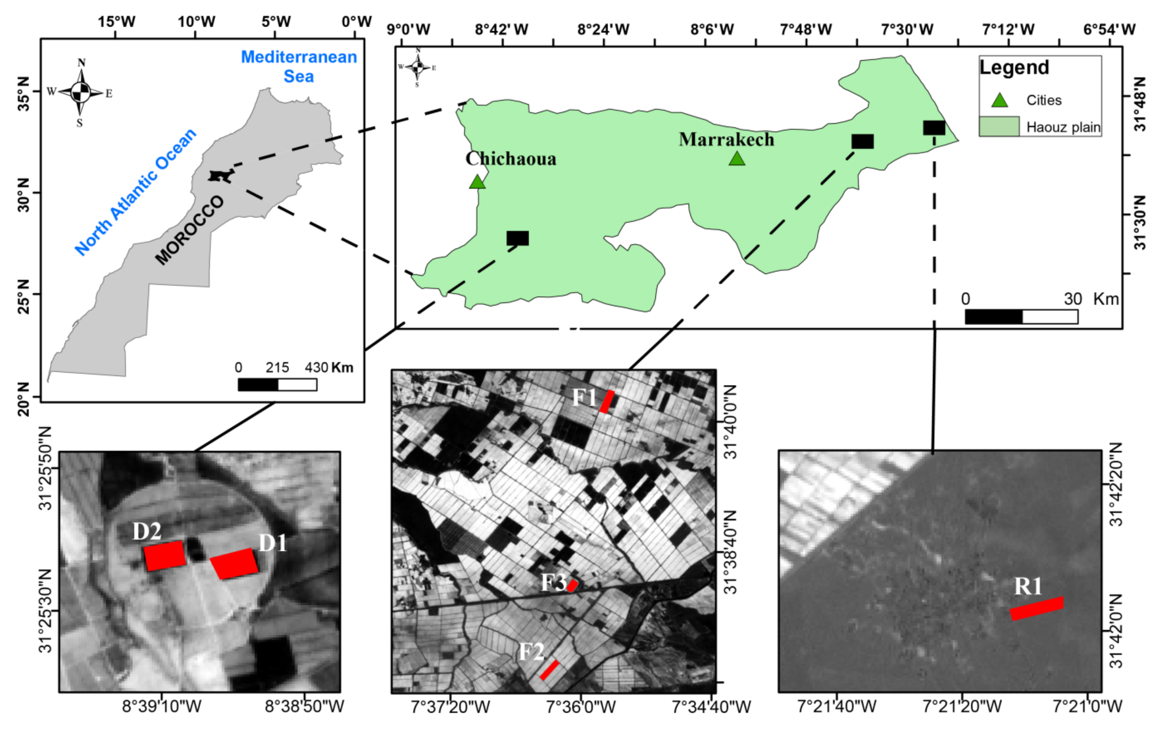
2.1. Study Region and Sites Description

The study area is located in the Haouz plain in central Morocco. The plain covers 6000 km² at 550 m above sea level. The irrigated area is of about 2000 km² in which the cereals represent 51% of the irrigated areas while rainfed wheat cover the non-irrigated part of the plain [41]. The climate is semi-arid Mediterranean characterized by high reference evapotranspiration (1600 mm/year) that exceeds the annual average precipitation (250 mm). The air humidity is about 50% and the temperature is characterized by large differences between winter and summer with a daily average ranging between 5 and 35 degrees Celsius [41]. Wheat crop is sown between November and January and harvested in May or June. The irrigation occurs from early winter to spring (December to April).

Five fields cropped with wheat within three experimental sites (Figure 1) with different irrigation techniques were monitored during several growing seasons:

Drip irrigation: two fields named D1 and D2, of 1.5 ha, located within a private farm near the city of Chichaoua (Figure 1) were monitored during two growing seasons (2016–2017 and 2017–2018). The sowing occurred in November, 25th and 27th and the harvest in May 15th and June 08th for 2016–2017 and 2017–2018 seasons, respectively. The soil texture is composed of 32.5% of sand and 37.5% of clay. It should be mentioned that wheat on D2 was impacted by very special growing conditions mainly the spread of weeds, particularly a type of wild thistles characterized by a horizontal structure. In addition, the seeds sowed in this field were a mixture of barley and wheat with higher density in D2 than D1, resulting in long stems that laid down under the effect of wind. Within this context, this field is used when considering in situ measurements to illustrate the effect of particular growing conditions on the accuracy of the irrigation retrieval. By contrast, it is discarded when using S1 SSM estimates because SSM retrievals are of bad quality due to these specific conditions as detailed in [17].

Flood irrigation: three fields named F1 (4.5 ha), F2 (4 ha) and F3 (2 ha) (Figure 1), located in an irrigated perimeter with flood irrigation [42] were monitored during different seasons. F1 was monitored during the season 2002–2003 while F2 and F3 were monitored during 2015–2016 agricultural season. The soil texture is composed of 47% of clay and 33% of loam. Please note that F3 was actually irrigated using the drip technique, but the farmer was applying massive amounts up to ~50 mm by events (8 events during the season), thus mimicking the flood irrigation technique [35]. Please note that F1, which was monitored during 2003 prior to the launch of S1, is included in this study in the evaluation section of the approach with in situ SSM data only (Section 4.2).

Rainfed field: One rainfed field of 1 ha, named R1 (Figure 1) is monitored during four agricultural seasons from 2014 to 2018 where the 2015–2016 season was bare soil (the wheat didn’t grow up by lack of rainfall). The soil texture is the same as the flood-irrigated fields. This field is used for an indirect evaluation of the irrigation retrieval method described in this study.

2.2. In Situ Data

2.2.1. Irrigation and Meteorological Data

An automatic weather station is installed near the fields of study. The weather station measures continuously the air temperature, solar radiation, relative humidity, wind speed and precipitation amounts with a time step of 30 min.

For the flooded irrigation fields, water is brought to the fields by a network of concrete channels with different sizes and flow rates. The amount of irrigation over each plot is determined from the flow rate of the canal knowing the opening duration of the channel through surveys in the field. For the drip-irrigated fields, irrigation amounts are measured by flowmeters. The owner of D1 and D2 uses the FAO-56 [40] approach to determine the irrigation amount and timing. A flowmeter was installed downstream of a valve that controls the distribution of water in the drip pipes [43]. On average, irrigation lasts about 105 min corresponding to an amount of 12.5 mm per event. At the beginning of the season, irrigation was applied every day during the first week of December (about 9 days after sowing just before emergence of wheat) with a total of 182.74 mm over D2 and 140.76 mm over D1. Such large amounts are generally applied by the farmers in the region in order to store water in the soil deep layers, to facilitate crop emergence and to avoid soil crusting [9,35]. Afterwards, events are programmed every two days (each period of irrigation) with amounts ranging from 7 to 22 mm for 2016–2017, and from 1.2 to 22 mm in 2017–2018. Irrigation was stopped around mid-April during 2016–2017 while no irrigation was applied after the beginning of February and March over D1 and D2, respectively, for the 2017–2018 season because of the wetter conditions of this season compared to 2016–2017. Concerning the flooded fields, four irrigation events were recorded over F1 with an amount of 60 mm each while over F2, 8 events of 64 mm are repartitioned on the period between the end of December and the end of April. For F3, the flowmeter was installed on January 21st while wheat already emerged at this date. 8 events were recorded form last January to the beginning of May with different amounts ranging from 23 to 50 mm. General information on irrigation practices over the irrigated fields (D1, D2 and F1–F3) are summarized in

Table A1. Irrigation general information of the irrigated fields.

Field	Technique	Irrigation Period	Amount’s Range (mm)	Number of Events	Seasonal Amounts (mm)
D1-2016-2017	Drip	Jan–Apr	8–22	16	239.26
D1-2017-2018		Dec–Feb	1.2–46	26	327.21
D2-2016-2017		Jan–Apr	7–19	29	373.02
D2-2017-2018		Dec–Mar	4–57	36	520.56
F1-2003	Flood	Feb–Apr	60	4	240
F2-2015-2016		Dec–Apr	64	8	512
F3-2015-2016		Jan–May	23–50	8	267.48

in the Appendix A.

2.2.2. In Situ Surface Soil Moisture

Measurements of surface soil moisture (SSM) were recorded using Time Domain Reflectometry (TDR) sensors located at a depth of 5 cm in each field. The sensors collected data every 30 min. D1 and D2 are equipped with a sensor under the drippers and a second is installed between two rows. The average of the two sensors is considered as the SSM of the field. Within the other fields (F1-F3 and R1), only one sensor is used. The calibration of these sensors has been carried out using the gravimetric technique (see [17,35,44,45,46] for details).

It should be mentioned that even if in situ SSM measurements are expected to be of better quality than C-band satellite estimates in particular when the vegetation cover is dense [17,47], in situ observations are also associated with errors, mainly of spatial representativeness. Indeed, the TDR measurements are point-scale while soil moisture may exhibit a significant spatial variability related to both variability in soil characteristics and heterogeneous irrigation amounts even at the field scale. In addition, for flooded fields, a point scale measurement can be misleading as irrigation of the field last several hours (irrigation is about 6 ha/day). Stated differently, irrigation may have not reached the point scale measurements while most of the field is already irrigated. For drip irrigation, in order to acquire a representative value of SSM, two probes installed under the dripper and between the row are used.

2.3. Remote Sensing Data

2.3.1. Sentinel-1 SSM Product

Sentinel-1 is a C-band synthetic aperture radar constellation composed of two satellites S1A and S1B launched in 2014 and 2016, respectively, by the European Space Agency (ESA). The operational imaging mode IW provides dual acquisitions in VV and VH polarizations. S1A and S1B scan the world in 175 orbits with a revisit time of six days [48]. The S1 products were downloaded from Data Hub website and processed using SNAP and OTB (Orfeo ToolBox) as described in [17].

SSM was retrieved based on the method described in [17] relying on the inversion of the water cloud model using the backscattering coefficient and the interferometric coherence derived from S1 data. The above-ground biomass derived from the interferometric coherence is used as vegetation descriptor in the model and hence, the SSM is derived from radar data using a brute-force method. The approach was validated using a large in situ database including the drip fields D1 from Morocco and other fields in Tunisia. Reasonable metrics were obtained with R = 0.74, RMSE = 0.06 m³/m³ and bias = 0.01 m³/m³. For more details about the approach, the reader is referred to the original paper [17]. Among the two incidence angles available on D1 (35.2° and 45.6°), SSM used in this study is derived from descending orbit #52 (35.2° incidence angle) since the lower incidence angles are more suitable for SSM retrieval [17,49]. D2 is not considered because the special growing conditions affected the geometry of the field and therefore affect the modeling of the radar signal leading to inaccuracy in the SSM retrieval (see [17] for more details). SSM for F2 and F3 is retrieved from orbit #45 (~40° of incidence angle) and from orbit #154 at 40° of incidence angle for R1. The VV polarization is chosen for all fields as it is less impacted by the volume diffusion within the canopy than VH [17,36,50]. Please note that S1 derived SSM is available every 6 days for D1 and R6 seasons 2016–2017 and 2017–2018 while it is available every 12 days for F2 and F3 during the season 2015–2016 as only S1A was in orbit. Obviously, remote sensing products were not available for F1 as the field was monitored during 2003.

2.3.2. Sentinel-2 Data

Sentinel-2 is an optical satellite composed of two constellations S2A and S2B launched by ESA in 2015 and 2017, respectively. With a revisit time of 5 days (using S2A and S2B), Sentinel-2 provides images composed of 13 bands among which the bands 4 and 8 are used in the computation of the Normalized Difference Vegetation Index (NDVI). The products corrected from atmospheric effects are processed by the CESBIO’s MAJA processor [51] and distributed as Level 2A products by the National Centre for Space Studies (CNES) via the open access platform (https://peps.cnes.fr/, accessed on 3 July 2021) or directly from the THEIA website (https://theia.cnes.fr/, accessed on 3 July 2021). The NDVI is computed for D1, D2, F2, F3 and R1 (seasons 2016–2017 and 2017–2018) from S2. For 2014–2015 season on R1, the MOD13A2 products used in [52] are also used here. The canopy cover fraction is derived from NDVI using the relationship developed by [53].

3. Methodology

Daily to seasonal irrigation timing and amounts are estimated at the field scale based on SSM data assimilated into the FAO-56 through a particle filter technique. The approach is implemented in three steps: (1) synthetic experiments are designed to assess the impact of the frequency of observation, the errors on SSM, and the a priori constraints on the irrigation scenarios for different irrigation technics (flooding and drip); (2) the method is evaluated using in situ SSM using three assimilation window lengths to mimic the revisit time of the available soil moisture products derived from existing and potentially future remote sensing sensors on polar orbiting satellites (3, 6 and 12 days); (3) the approach is evaluated using SSM products derived from S1 data.

3.1. FAO-56 Dual Crop Coefficient

A land surface model is used for the daily prediction of the soil water budget. The land surface model used in this study is the FAO-56 model with the dual crop coefficient approach [40] because it has been extensively calibrated and used to predict evapotranspiration of wheat in the region of study [45,53,54,55]. A brief description of the model is provided in the Appendix A. The model is run at a daily time step forced by the precipitation amounts and meteorological data including air temperature, air humidity, wind speed and solar radiation. Vegetation variables are the canopy cover fraction and the crop coefficient. The crop coefficient K_cb is estimated from S2 NDVI using the relationship proposed by [54]. Finally, soil parameters include wilting point and field capacity derived in this study from field measurements carried out on site [35,45,54].

The predicted surface soil moisture ($SS{M}_m$) is derived from the surface soil water depletion D_e:

$$SS{M}_m={\theta }_{fc}-\frac{D_e}{Z_e\ast 1000}$$

(1)

where ${\theta }_{fc}$ is the field capacity and $Z_e$ the soil evaporation layer depth.

The depletion D_e is given by the daily water balance equation of the surface soil layer for the exposed and wetted soil fraction $f_{ew}$ [40]:

$$D_{e,i}=D_{e,i-1}-P_i-R_{o,i}-\frac{I_i}{f_w}+\frac{E_i}{f_{ew}}+T_{ew,i}+D{P}_i$$

(2)

where $D_{e,i}$ is the depletion of the day i, $P_i$ the precipitation, $R_{o,i}$ the precipitation runoff, $I_i$ the irrigation, $E_i$ the evaporation, $T_{ew,i}$ the transpiration from the exposed and wetted soil fraction, $D{P}_i$ the deep percolation and $f_w$ the fraction of soil surface wetted by irrigation.

3.2. Particle Filter Approach and Implementation

A particle filter approach is implemented for the assimilation of SSM into the FAO-56 model in order to retrieve irrigation water amount and timing. The most popular data assimilation technique used in geophysical problems is the Kalman filter and its variants, an optimal solution when the problem is linear and the posterior density is Gaussian. Some variants of Kalman filters are developed to solve some nonlinear problems as well, such as extended Kalman filters, but with a Gaussian posterior density function. However, when these two conditions (linearity and Gaussianity) are not satisfied, the performance of the variants can be limited [56]. In this case, the particle filter technique was shown to be better suited than Kalman’s similar approaches [57,58].

Particle filters are a sequential Monte Carlo data assimilation technique implementing a recursive Bayesian filter [59]. They are powerful and flexible techniques that can describe a wide range of problems [60], in particular they are not limited to Gaussian distribution, unimodal solution and linear problems [60,61,62]. The principle of particle filters can be summarized in two steps [63]: prediction and weights update. In the first step, a set of particles of the analyzed variable with equal weights is generated. The particles are propagated in the state space using the model (state equation) to generate predictions of the state variable until a new measurement (or observations) is available. The predictions are compared then to measurement and the weights are actualized based on the adequacy of predictions with the current observations thanks to the likelihood function [64].

In this study, the algorithm is run on assimilation windows of a duration equal to the data revisit time (6 days or 12 days for S1 SSM products depending on the site). A sensitivity analysis to the revisit time is conducted using in situ measurements by varying the windows length from 3 days (revisit time of SMOS product) to 12 days (revisit time of S1 when S1A only was available before 2016). An ensemble of N particles is stochastically generated at the beginning of each assimilation windows. Each particle is associated to an irrigation scenario generated stochastically.

The amounts and the day of irrigation (timing) are generated stochastically using a uniform distribution as no information are available on both variables. For flood irrigation, the minimum time between two irrigations is defined to a value of n days (a sensitivity analysis to this constraint is carried out in the Section 4). Indeed, flooding is constraint by the channel network bringing water to the field and by available workforce leading to an irrigation event every 15 days at best. The amount ranges between 20 and 80 mm of water which are typical values applied for flooding irrigation. For drip irrigation, the irrigation is applied with values ranging from 0 to 40 mm and n (the minimum time between two irrigations) is defined to two days.

The set of particles evolves using the FAO-56 from the beginning to the end of the window where an observation is available following:

$$x_i^k=f\left(x_{i-1}^k,I_i^k,u\right)+{ϵ}_i^k$$

(3)

where $x_i^k$ is the analyzed variable, (the water depletion only in our study; see Equation (2)), f is the FAO-56 model equation (Equation (2)), $I_i^k$ is the corresponding irrigation scenario, u contains the model parameters (FAO-56 parameters, see

Table A2. The FAO-56 parameters used for the studied fields.

	D1–D2	F1–F3	R1
$Z_e$ (m)	0.05	0.05	0.05
$Z_{r max}$ (m)	1.2	1.2	1.2
REW (mm)	8	9	9
${\theta }_{fc}$ (m3/m3)	0.26	0.37	0.37
${\theta }_{wp}$ (m3/m3)	0.07	0.17	0.17

in the Appendix A) and ${ϵ}_i^k$ is the modeling error.

After predicting a set of SSM states (N values) corresponding to the ensemble of irrigation scenarios, the particle that most closely matches the observation is sought. This is achieved by computing the likelihood of the measurement y (SSM observation) giving the particle x using the probability density function (PDF) described by:

$$p\left(y_i|x_i^k\right)=\frac{1}{\sqrt{2\pi \det \left(C_V\right)}}{e}^{-0.5\ast {\left(y_i-x_i^k\right)}^T\ast C_V^{-1}\left(y_i-x_i^k\right)}$$

(4)

This is a simplified form (adaptation to our case where only one observation is assimilated per window) of the probability density function obtained from Bayes’ theorem in [65]. The likelihood is driven by the difference between the measurement and a given particle $\left(y-x^k\right)$. The closer the particle is to the measurement, the higher the likelihood. Another important parameter is the error covariance of observations $C_V$ that controls the weight distribution. A small $C_V$ will provide very high weight to the particles closest to the measurement [31]. As SSM only is assimilated here,$C_V$ is a scalar. Its value is set to the error on the SSM products assimilated in this work.

The likelihood is translated into weight by normalizing with the sum of all the particles’ likelihoods, so that the sum of the weights equals to 1:

$$w_i^k=\frac{p\left(y_i|x_i^k\right)}{{{\displaystyle \sum }}_{k=1}^{N}p\left(y_i|x_i^k\right)}$$

(5)

$w_i^k$, the weight of the particle k at time i takes a value between 0 and 1 and N is the number of particles. N has been defined to 1000 in this study in order to achieve a good performance [61,66,67].

After several assimilation windows, it is likely that a single particle will have a weight close to 1 while all the other particles will end up with weights close to 0. For example, it is shown by [68] that after a few iterations, all the weight is concentrated on one particle, even using a relatively simple system. This is known as particle degeneracy [56,63,69]. To overcome this problem, a resampling of the particles must be carried out to eliminate particles with low weight and duplicate those with high weights. Several particle resampling methods have been proposed [70,71,72,73,74,75,76] showing their effectiveness in improving the performance of the particle filter algorithm. In this study, the “systematic” method (also called “stratified” on some references) introduced by [77] is used. The authors argued that greater accuracy can be achieved using this method according to sampling theory. It is also preferred because of its simple implementation [61,70,75]. Degeneracy of particles is measured using either the effective particle number [78] or the entropy [79]. Here, the resampling of the particles is performed based on the effective particle number:

$$N_{eff}=\frac{1}{{{\displaystyle \sum }}_{k=1}^N{(w_i^k)}^2}$$

(6)

The ratio $N_{eff}/N$ measures the importance of the particle’s contribution to the state estimation. When the ratio is ~1, this means that all the particles contribute equally ($w_i^k~\frac{1}{\mathrm{N}}, \forall k$). In contrast, $N_{eff}/N$ ~0 means that one particle has a very high weight while the others are close to nil. In this study, when the ratio $N_{eff}/N$ is less than a fixed threshold of 0.5 [80], the resampling is performed.

Finally, the particles and their weights can be used in different ways to extract the best state estimation (SSM in our case). Here the particle with the highest weight is considered as the best state estimate and translated afterwards into the irrigation amounts and timing assuming that the best estimated SSM state corresponds to the best irrigation amounts and timing. The algorithm is applied over all the growing season from sowing to harvest.

3.3. Experimental Design

3.3.1. Synthetic Experiments

The objective of the synthetic experiments is to investigate the sensitivity of the algorithm to some important parameters of the approach including (i) errors on the SSM measurements, (ii) window length or observation frequency and, (iii) irrigation timing constraints. For this purpose, a set of synthetic observations of SSM were generated using the FAO-56 model by perturbing the model’s parameters. Two experiments were carried out, one for flood and a second for drip irrigation. For the flood experiment, 6 irrigation events of 60 mm were applied throughout the season with an interval of 15 days between two successive events, which corresponds to the typical frequency of the classical flooding technique. For the drip experiments, irrigation data recorded on D1 during the 2016–2017 growing season were used.

Errors on SSM: The final objective of our study is to rely on remote sensing SSM products. Products derived from microwave remote sensing are overall retrieved with an error [17,39,81,82]. This error is assumed to decrease the approach performance and thus results in errors in the state estimation. To assess the effect of error on the proposed approach, five levels of error are investigated in this study: 0 (no error), 0.02, 0.04, 0.06 and 0.1 m³/m³. This frames the error value of most satellite products as well as the error threshold that defines good quality of SSM products (0.04 m³/m³; [83]). Errors are first randomly generated by a Gaussian PDF with a mean equal to zero and a standard deviation equal to the level of error, and then added to the synthetic observation data set.

Window length: It is the frequency of observation availability. In this study, the window length corresponds to the revisit time of the satellite, which implies that only one observation is available per window. The effect of this parameter is important given that the weights are kept constant along the window, which means that a large window (large difference between two successive observations) is less accurate in tracking the state variable than a small window. In the context of this study: irrigation estimation, a long window will miss the effect of irrigation because the soil dries out after a long period of time. Therefore, if the following SSM observation is low, the algorithm assumes that no irrigation has taken place. In this study, we considered the investigation of three windows, being 3-, 6- and 12-day long.

Irrigation timing constraints: The aim is to evaluate the effect of adding some constraints on the timing of irrigation application in the case of flood irrigation. It consists of adding a condition to the approach when it detects an irrigation event. A 5-day constraint for example implies that when an event is detected, no irrigation will take place within the next 5 days. For this study, two constraints of 5 days and 10 days were tested, in addition to no constraint, i.e., the approach can retrieve irrigation events every day.

For each set of algorithmic parameters (SSM error, window length and timing constraint), the data assimilation is run 10 times to take into account the effect of random errors and particle distribution.

3.3.2. In Situ SSM Assimilation

As a first step before using remote sensing-derived SSM products, the irrigation retrieval approach is tested using in situ measurements of SSM. The algorithm is evaluated over three (3-, 6- and 12-day) window lengths to mimic the temporal resolution of the available SSM products over the entire growing season. The in situ data base is composed of ten growing seasons, including 4 drip-irrigated, 3 flood-irrigated and 4 rainfed seasons (one of which 2015–2016 being bare soil). For the four rainfed seasons, the same irrigation routine (amounts, particles…) as the flood technique is applied but without any constraint on the timing for the three windows.

3.3.3. Satellite SSM Assimilation

The assimilation of remotely sensed SSM products derived from S1 is constrained by the acquisition configuration of S1. For D1 and R1, SSM products are available during both the 2016–2017 and 2017–2018 seasons with a revisit time of 6 days as both S1A and S1B satellites were used. The assimilation window is therefore set to 6-day for both fields during both seasons. For the flood irrigated fields F2 and F3, observations are available every 12-day since only S1A was into orbit during the 2015–2016 season. As already stated, D2 was discarded from the analysis because of the very specific growing condition of this field.

3.4. Statistical Metrics

The statistical metrics used in this study to assess the performance of the proposed approach are as follows:

Drip irrigation: Small amounts of water are applied frequently resulting in smooth SSM dynamics making difficult to retrieve daily irrigation values [32]. For the flood irrigation, large amounts of water, of 60 mm on average, are applied every 2 to 3 weeks. This leads to a strong dynamic of soil moisture and contrasted soil moisture conditions that are easier to catch with a SSM observations every 6 days than the much smaller amounts applied using the drip irrigation technique that maintain soil moisture at high level. For this reason, the performance of the algorithm on the dripped sites is evaluated by accumulating irrigation amounts by 15 days following [35]. Statistical metrics including R, RMSE and bias are therefore computed between actual (true) and estimated 15-day cumulative amounts.

Flood irrigation: The metrics computed for the flooding technique are intended for a daily evaluation of the irrigation estimate. The percent bias (Pbias) is calculated to measure the over/under-estimation in terms of amounts. The Total Positive Rate (TruPosRat) is the ratio of the number of irrigations detected within a specified range from actual irrigation (time difference from the actual events) to the number of actual irrigations events over the season. Here, the 4-day range was chosen as the 3-day range provided with much lower statistical metrics while the 5-day range did not improve significantly the scores (not shown). TruPosRat allows evaluating the irrigation estimates in terms of the timing (day of detection). Finally, in order to evaluate the underestimation or overestimation in terms of the number of events, the ratio between the estimated number of irrigation events and the actual number of events is computed (named irrigation events ratio and abbreviated to IrrigEvntRat hereafter).

Finally, the estimated seasonal amounts (sum) of each plots and seasons, including the rainfed seasons, are compared to the measurements.

4. Results

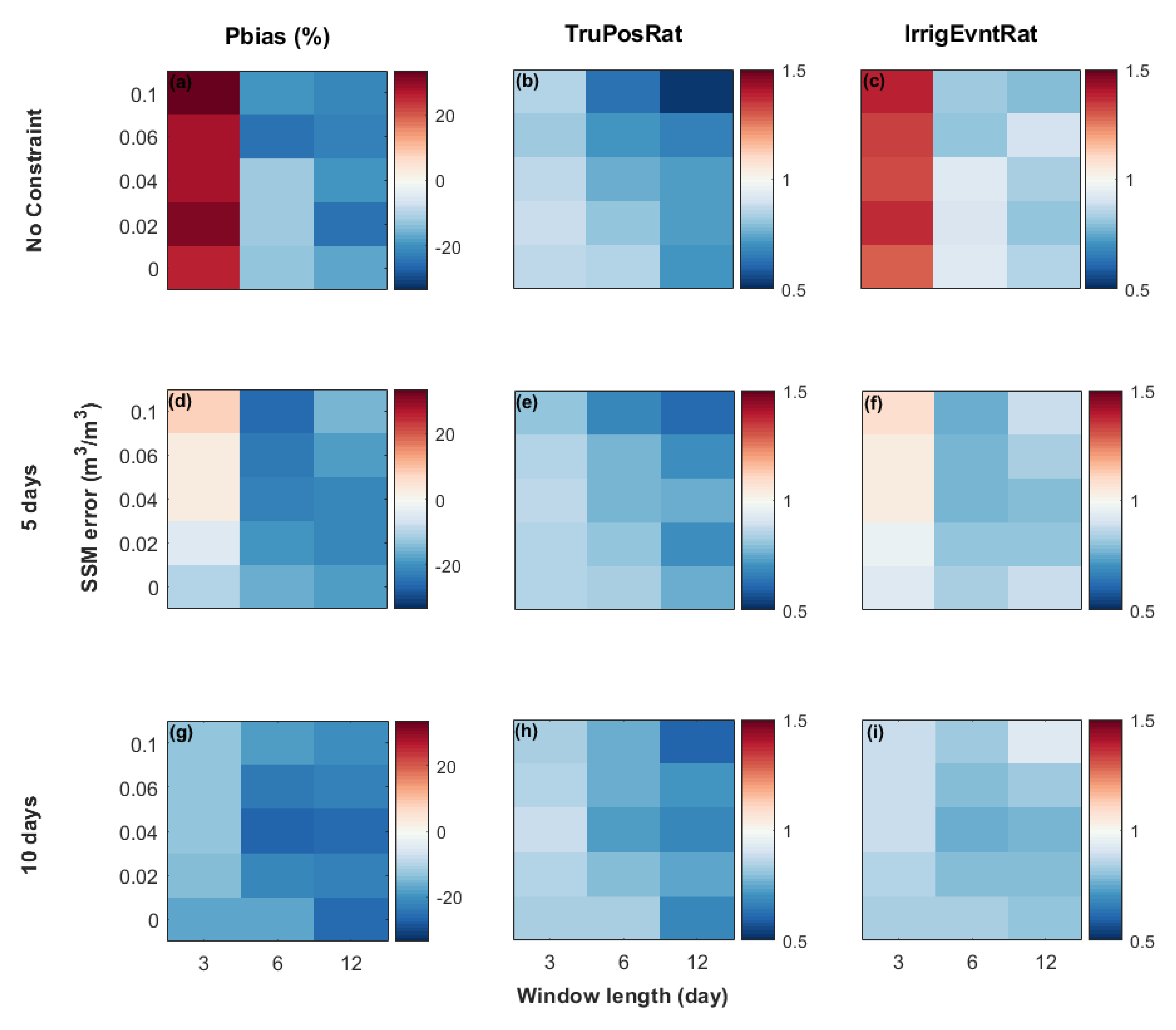
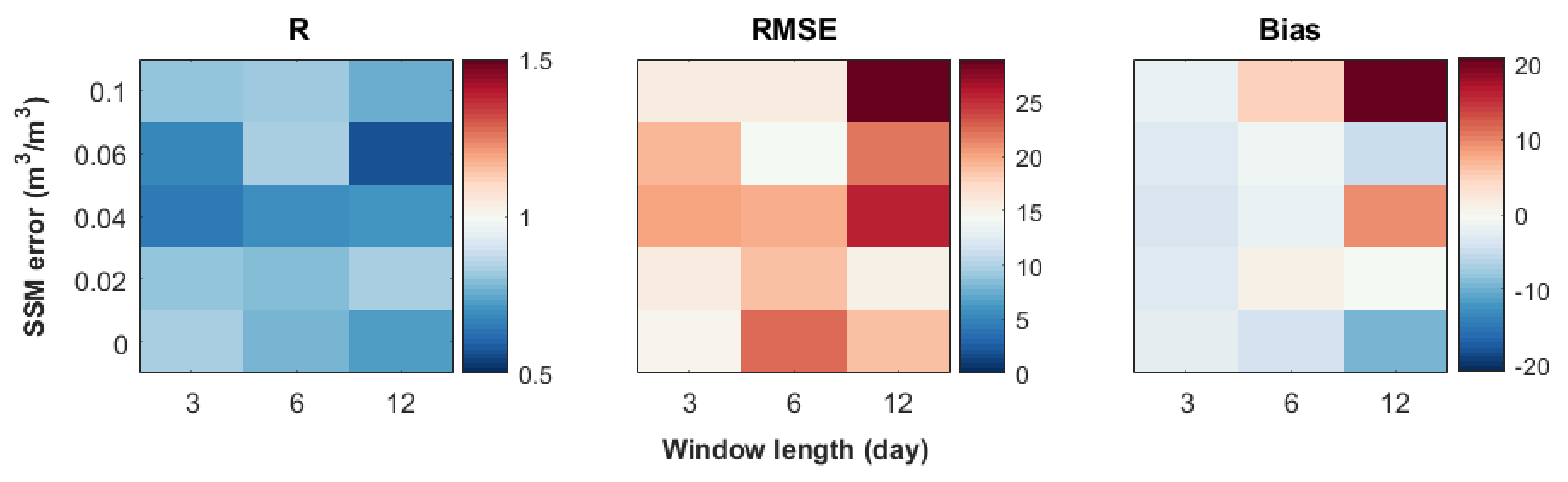
4.1. Synthetic Experiments and Sensitivity Analysis

4.1.1. Flood Irrigation

Figure 2 summarizes the results of the synthetic experiments for the flood irrigation technique for the three window lengths. Figure 2a–c represent, respectively, the Pbias, the TruPosRat and the IrrigEvntRat when there is no constraint on the timing of irrigation. Figure 2d–f and g–i are the same as Figure 2a–c but applying a constraint of 5 days and 10 days between two irrigation events, respectively.

For a 3-day revisit time, the Pbias ranges between −25% and 33%. An overestimation is only observed when no timing constraint is applied between two irrigation events. This overestimation is attributed to the false detection of two irrigation events during rainy period also illustrated by the IrrigEvntRat values of 1.28.. The Pbias is significantly lower with the application of a 5-day constraint with a value of 25%; the IrrigEvntRat also improved going from 1.28 to 1.00 while a 10-day constraint improved only slightly the metrics. The number of irrigations detected around the actual irrigation day within a 4-day interval is more than 80% (TruPosRat = 0.8) for all cases and errors. With 5- and 10-day constraints, close performance is always obtained. The best TruPosRat values is 0.88 corresponding to a 2% error on SSM but close values are obtained for error from 0% to 4% (TruPosRat = 0.86). By contrast, the lowest TruPosRat equal to 0.80 is observed when the observation error is 10% and the constraint is 5 days.

By contrast with the 3-day window, an underestimation of the amounts is observed whatever the error or the timing constraint for a 6-day window (IrrigEvntRat values of 0.88). This is due to an undetected event rather than an underestimation of the events amounts (not shown). A further analysis of the time series pointed out that one event was not detected because two rainfalls for a total of 35 mm were recorded at the time of the irrigation event. A low difference between the two SSM observations around the event in addition to the presence of an important rainfall prevented the approach from identifying a need for additional water in this period. Regarding the error on SSM, Pbias is less than −12% up to an error of 4% and it drops to −20% for higher errors due to an underestimation of both irrigation amounts and of the number of events (as clearly shown by the IrrigEvntRat). Likewise, IrrigEvntRat is almost stable up to an error of 4%, around 0.93 meaning that almost all the irrigation events are detected on time when no timing constraint is applied and above 4% it drops to 0.8 (for errors of 6 and 10%). In terms of timing, TruPosRat decreases from 0.85 when there is no error on the SSM to 0.63 when considering a 10% error. Between 2 and 4% of error, a likely error range for existing products derived from SMOS [81,82] or S1 [17,39], the TruPosRat is between 0.8 and 0.75 meaning that 75–80% of the irrigation events are detected on time. Finally, the worst metrics are obtained for the 12-day revisit time. This was expected considering the rapid dynamic of SSM that can dry out in a couple of days and well before the next available observation with a revisit time of 12-day. For instance, a loss of 17% and 5% in terms of TruPosRat is observed with regards to a revisit time of 3 and 6 days, respectively for an error of 4%. As for the 6-day window, adding a timing constraint has almost no impact on the metrics. When no constraint is applied, a clear decrease of the TruPosRat is observed when going from 0% error (0.71) to 10% (0.52). Likewise, at 5 days, the minimum value is 0.61 obtained at 10% error while it remains above 0.7 for the other error levels.

As a conclusion, these results demonstrate: (1) the importance of constraining the timing of irrigation for the flooding technique in particular for the shorter window of 3 days; a 5-day constraint being a good trade-off; (2) shorter windows allow better identification of irrigation events, especially in complex conditions where irrigation overlaps with significant rainfall events.

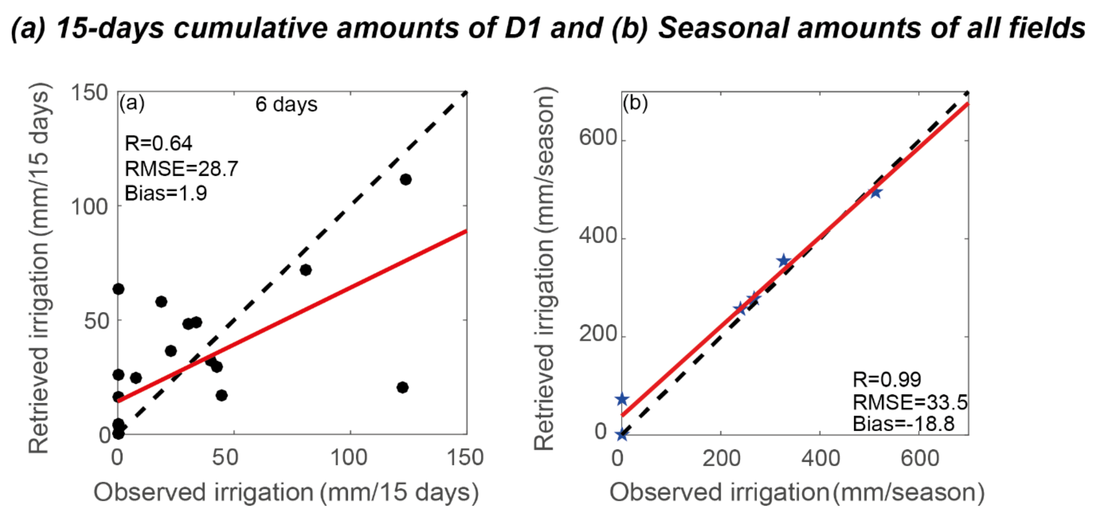
4.1.2. Drip Irrigation

The results of the synthetic drip irrigation experiment are shown in Figure A1 in the Appendix A. The overall behavior of the results is not as conclusive as for the flood irrigation. Yet, for an error <2%, the metrics are good for the three window lengths, while above 4%, no overall behavior is observed, as 10% error yields comparable results to the <2% error. The bias is slightly better for a 3-day revisit time than with 6-day, but both shorter revisit times outperformed the 12-day one. The loss of performance is also clear at 12 days for error above 6% as expected. Indeed, the highest RMSE and bias are obtained for the 12-day window at a 10% error on SSM (RMSE = 28.65 mm and bias = 21.71 mm).

As for the flooding technique, the 3-day revisit time window performs better than the 6- and 12-day windows time steps. Likewise, very accurate estimation of SSM is needed for a good irrigation timing retrieval, in particular when irrigation events are concomitant with rainfall. This may be explained by the limited information provided by SSM as the upper soil reservoir may dry out quickly all the more in the semi-arid sites considered in this study.

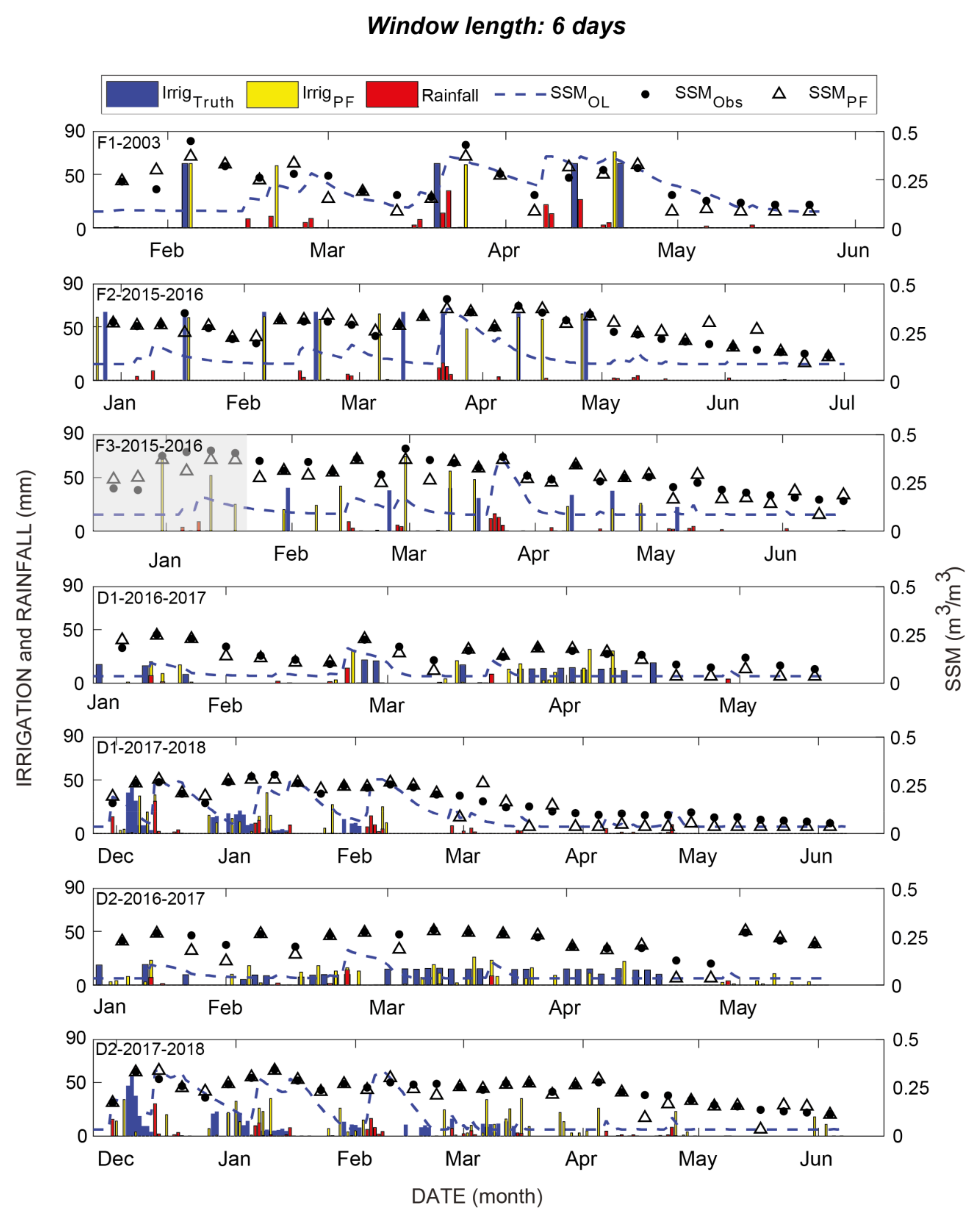
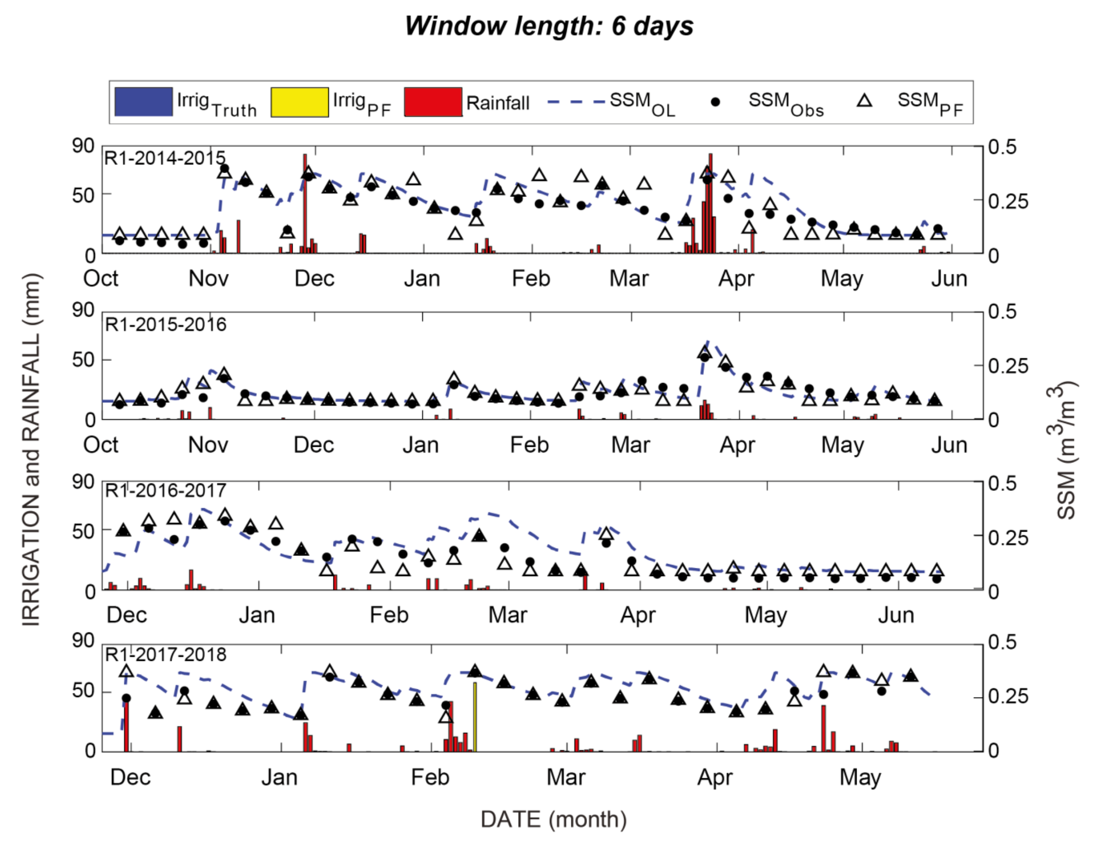
4.2. Assimilation of SSM In Situ Measurements

In this section, the retrieval of irrigation using in situ SSM measurements with a revisit time mimicking potential satellite overpasses of 3-, 6- and 12-day windows are presented. Figure 3 displays the time series of observed, analyzed and open-loop (without data assimilation meaning no irrigation water inputs are applied) SSM together with measured and retrieved irrigations with a 6-day revisit time for the irrigated and the rainfed fields, respectively. Figure A2 in the Appendix A is the same as Figure 3 but for the rainfed field. In addition, Figure 4 shows the statistical metrics as a function of the revisit times of 3, 6 and 12 days.

The open-loop (with no irrigation inputs) obviously failed in reproducing the SSM observations while the analyzed SSM (corrected by assimilating SSM observations) are much closer to the observations. In terms of irrigation retrieval, among 20 observed events considering the three fields, 17 irrigation events were reasonably detected within a delay ranging from 1 to 5 days. For instance, on field F2, the eight observed irrigation events are detected within 0 to 6 days around the real time of application and among them 6 within 0 to 2 days. Likewise, annual amounts are in good agreement with the actual events for F1 and F2 (Figure 5) with an average absolute difference of 3.5 mm (5.8%) and 5.8 mm (9.2%) over F1 and F2, respectively, while it is about 44% on F3. On this field (F3), irrigation practice is very specific as already underlined and the amounts are estimated by subtracting the previous metering to the observed value registered by the flowmeter at the day of survey. This means that the timing of irrigation as well as the amount are very uncertain if surveys are not carried out on time. Finally, the seasonal distribution of events is also in agreement with irrigation practices in the region as no event was detected during the senescence period when the soil moisture was low. By contrast, some false detections are observed (end of February on F1; start of the season on F3) and some events were missed by the retrieval algorithm. For the latters, a finer analysis pointed out the important role of rainfall that drastically impacts the irrigation retrieval when irrigation input is concomitant with a rainfall event. Indeed, rainfall can refill the thin superficial layer such as no irrigation input is necessary to match the SSM observation. On F1 for instance, the third event is not detected as two rainfall events are registered around the irrigation for a total amount of 35 mm. A similar remark can be drawn for the undetected event observed at the end of March on F2. On F3, at the beginning of the growing season (see the shaded area on Figure 3), three events are detected while no observation was available during this period because the flowmeter was installed on January 21st. Nevertheless, large irrigation events at this time of the season are in-line with the farmers practices that water the fields in order to favor emergence and to avoid soil crusting.

For the drip irrigated fields D1 and D2, the seasonal timing of the detected events is also in-line with the agricultural practices of the region as there is no retrieved event during senescence. This is particularly prominent on D1, in particular during 2017–2018 when the farmer stopped irrigation as early as February. By contrast, some false detections are observed on D2 at the end of the two seasons. The detected events are consistent with the SSM values close to field capacity during the first season at this time. These high values of SSM were related to the very specific growing conditions on this field with dense adventices and the wheat stems that were laid down by high winds from mid-April. This probably created a shielding layer that limited soil evaporation. The false detection at the end of the second season could also be related to the error on the SSM observations leading to a spurious slight increase between two observations. A strong underestimation of the high amounts (140.76 mm in D1 and 182.74 mm in D2) that were applied during the first week of December (see Section 2.2.1) 2017 is also observed on D1 and D2. This is related to the limitation already underlined of relying on SSM observations only to retrieve irrigation: the superficial layer is refilled by the first water input and the subsequent events have no impact on the SSM that reached the field capacity/saturation value.

By contrast with the irrigated fields, open-loop SSM time series are obviously in good agreement with the observations for the rainfed field R1, apart during the 2016–2017 growing season and around early April of the 2014–2015 season (Figure A2). The best agreement between the observations, open-loop and analyzed SSM is observed during the bare soil conditions of the season 2015–2016 as wheat didn’t grow up by lack of rainfall. During the four growing seasons, only one false event is detected around mid-February during 2017–2018 season providing an additional assessment of the method.

On average for the flood irrigated fields, the shorter the revisit time, the better the detection of irrigation events (Figure 4a–c). For a 3-day revisit time, more than 75% of the irrigation events (TruPosRat = 0.75) are detected with a time shift with regards to the real application lower than 4 days and even up to 94% for F2. By decreasing the temporal resolution, the percentage of detection drops to 67% and to 58% on average for 6 days and 12 days, respectively. Pbias and IrrigEvntRat provide with similar information as both reflect mainly the false detection. For instance, the high Pbias value on F1 for a 3-day revisit time is associated to the false event detected after mid-February (see Figure 3) in agreement with the IrrigEvntRat value above 1 (IrrigEvntRat = 1.1). Likewise, the high IrrigEvntRat value obtained at F3 is the result of the detection of some false irrigation events, although the Pbias remains low due to the amount underestimations on average. By contrast, the IrrigEvntRat is closer to 1 for a 6-day revisit time on F1 because a missed event is compensated by a false detection. The worst metrics are obtained for a 12-day revisit time because of the quick change in soil moisture of the upper soil layer: an irrigation event occurring at the beginning of the 12-days windows can be missed because the superficial soil layer can dries out totally before the next available observation as already commented. This typically occurred for the last 4 events applied on F3 when the 12-day observation does not track changes in SSM (not shown). Nevertheless, reasonable results are obtained. For instance, the number of detected irrigation events is the same as for a 6-day revisit time for F1 and F2 while an underestimation on F3 is observed because of missing events (see above). By increasing a threshold considered for a good timing detection from 4 to 5 days, TruPosRat scores improved to 0.70, 0.74 and 0.62 for F1, F2 and F3, respectively, instead of 0.59, 0.68 and 0.48 for 4 days.

The results of 15-day cumulated amounts over the drip irrigated fields are presented in Figure 4d–f. Similar performance is obtained for both 3-day and 6-day revisit times with reasonable RMSE and bias. Lower statistical metrics are obtained for the 12-day window with an acceptable RMSE. The most notable outlier is highlighted in Figure 4d–f. It corresponds to the underestimation observed at the beginning of the 2017–2018 seasons. The underestimation in December 2018 is noticeable for all the windows while the underestimation in January is only significant for a 12-day window. In a second step, data of D2 during 2017–2018 season are discarded given the high SSM values at the end of the season (especially the 2017–2018 season) due to the very specific growing conditions observed on the field. The results are significantly improved for the three windows as shown in

Table 1. Statistical metrics for the 15-day cumulative amounts over the drip irrigated fields when discarding data of D2 during the 2017–2018 season, for the three 3-, 6- and 12-day window lengths.

	3 Days	6 Days	12 Days
R	0.77	0.74	0.65
RMSE (mm/15 days)	23.6	24.8	27.1
bias (mm/15 days)	0.24	2.3	2.3

: the best performance is obtained for a 3-day revisit time but RMSE and bias are still reasonable at 6 days and, to a lesser extent, 12 days.

Finally, the estimated seasonal amounts are plotted against observation for the three window lengths at Figure 5. While it has been observed that the intra-seasonal dynamic of the retrieved irrigation event may present some scattering with the observations, the seasonal amounts are remarkably well estimated for the three window lengths. At 3 days, the noticeable outlier corresponds to an overestimation over the rainfed field R1 during season 2017–2018 when a false irrigation event is detected. For a 6-day window, the estimation is still accurate with a slight loss of statistical metrics with regards to a 3-day revisit time. In addition to the outlier already observed at 3 days, another one is detected that corresponds to the 2017–2018 season over D1 where several events were missed at the beginning of the season. The estimation accuracy dropped for a 12-day revisit time underlining the difficulty of correctly detecting not only the timing of events but also the amounts of irrigation when the available observation frequency is low.

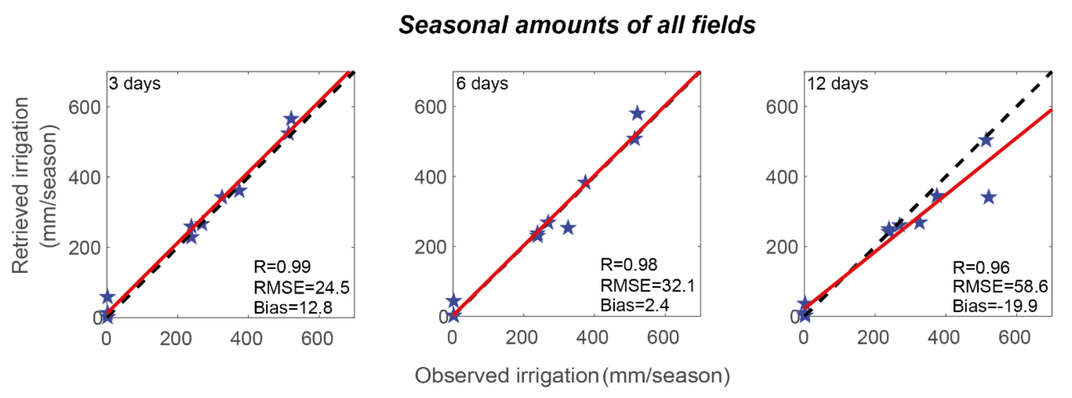
4.3. Assimilation of Sentinel-1 Derived SSM

Figure 6 is the same as Figure 3 and Figure A2 but the irrigation retrievals are based on the SSM products derived from S1 data. The statistical metrics are reported in

Table 2. Statistical metrics of the estimated irrigation over the flood irrigated F2 and F3 when assimilating S1-derived SSM for a 12-day window.

TruPosRat (4 Days)		TruPosRat (5 Days)		IrrigEvntRat		Pbias
F4	F5	F4	F5	F4	F5	F4	F5
0.50	0.44	0.63	0.56	1.15	1.09	−3.14	3.98

for the flooded fields. Figure 7a displays the scatter plots of the 15-day cumulative amounts for the drip irrigated fields and Figure 7b reports the estimated seasonal amounts against observation for all fields. Data with a 6-day revisit time were available for D1 and R1 during 2016–2017 and 2017–2018. By contrast, only one observation every 12 days was available over F2 and F3 in 2015–2016 as already underlined.

The results obtained with the S1 products are close to the one based on in situ measurements to some extent: (1) the SSM open loop (without irrigation inputs) does obviously not match the observations while the analyzed SSM is in good agreement with the SSM S1 products for irrigated fields, and to a lesser extent, for the rainfed seasons as well; this means that the algorithm is able to identify at least one irrigation scenario to be able to match the observed SSM; (2) the overall distribution of the irrigation events during the season are properly reproduced; see for instance D1 where almost no irrigation is detected after the farmer decided to stop irrigation apart from some false events detected in early March in 2017–2018 occurring concomitantly with rainfall. This is attributed to an overestimation of the retrieved SSM with regards to in situ data at this time; (3) there are some compensations between some undetected events and some others that are falsely detected leading to acceptable retrieved seasonal amounts; the false detection in early March on D1 2017–2018 (see above) compensates for the underestimation of the retrieved irrigation amounts during the early stage of the season; likewise, false events detected at the end of season on F2 and F3 were compensated by the undetected event in March; (4) finally, only one irrigation is detected for the rainfed field during the 2017–2018 in line with the results obtained by using the in situ data.

The overall statistics are only slightly lower than those obtained with the in situ observations. The 15-day cumulative amount for the drip field D1 is retrieved with an R of 0.64 (R = 0.72 when using in situ SSM with a 6-day revisit time); RMSEs are close and bias is even lower. The irrigation retrieval is even better with S1 data for D1 during the season 2016–2017 (R = 0.80 using S1 SSM vs. 0.77). By contrast, the results obtained on F2 and F3 suffered from the 12-day revisit time of the available SSM products in line with the results obtained previously both based on the synthetic experiment and on the in situ SSM using the same revisit time. Overall, the detected events at the start and at the end of the actual irrigated period are in good agreement with the actual irrigation timing and amounts while some false events are detected at the end of the season in May and June. In addition, irrigation events are not properly detected in March when the crop cover is fully developed. This mainly originated from issues related to the retrieved SSM product at this time. The backscattering mechanism is characterized by a significant contribution of the interaction between the soil and the canopy that the simple water cloud model used to retrieved SSM was not able to simulate correctly [17] leading to poor SSM quality. On average, ~50% of the irrigation events can be detected in a range of 4 to 5 days around the actual irrigation date with a limited Pbias of ~4% and only one false event detected over the season (Table 2).

5. Discussion

Even though some limits are highlighted in relation to the quality of the SSM products, the reasonable statistics obtained by assimilating the S1 products, close to those obtained by using in situ SSM demonstrates the feasibility of irrigation retrieval using high-resolution soil moisture products derived from S1 when compared to other studies. For example, in the study by Zappaet al. [32], the seasonal dynamic of irrigation is well reproduced but the weekly and seasonal amounts retrievals suffered from significant biases. As already shown by other authors [32,35], the retrieval of the exact timing and the amount of irrigation events is difficult for drip irrigation. Our statistics are close to those of Dari et al. [29] who obtained a Pearson correlation coefficient of 0.69 on average for 5-day cumulative amounts. The seasonal amounts statistics also compared well with the results obtained using in situ measurements and using a thermal-based approach in [35]. Interestingly enough, the good seasonal statistics are sometimes obtained because some missed events are compensated by some false detections at the seasonal scale as already shown by [35].

One important point highlighted by this study is the importance of the revisit time as the best retrieval performance are obtained for a 3-day revisit time. The performance decreases for higher revisit time because the surface layer can dry out within a few days, in particular for the semi-arid climate of our study sites. This is in line with the work of [32] who showed that, on average, 81% of the observed events are detected with a revisit time ranging from 1.5 to 4 days while only 58% of the irrigation events were correctly detected with the 6-day revisit of combined S1A and S1B on 3 plots in Montpellier by [37]. Le page et al. [38] reported that the detection of irrigation events can be difficult when it occurs 5–6 days before S1 acquisition for the same reason of quick soil drying. Likewise, Zappa et al. [32] encountered the same difficulty in detecting all events, especially in some periods where the revisit time of SSM observations goes above 8 days in-line with the results obtained in this study considering a frequency of observations of 12 days. These results highlights that a satellite constellation with a 3-day revisit time would be relevant for irrigation detection at the field scale, as will be provided in a near future by the Copernicus constellation after the launch of Sentinel-1C planned in 2022 [84]. This work also showed that irrigation events occurring concomitantly with rainfall may be missed, consistent with the work of [20,30,38]. Indeed, the superficial layer may be refilled totally with rainfall only. In that case, the irrigation amount cannot be “seen” by the superficial reservoir information alone, provided by SSM observations.

Finally, the question arises of the genericity of the proposed approach applied here on wheat crops only. The method relies on three main assumptions that are discussed: (1) with regards to the work of [38] relying on relative change between observed and predicted SSM, absolute values of SSM are used in this study meaning that the soil hydraulic characteristics must be known as they are needed to determine the soil parameters of the FAO-56 approach (see Appendix A); (2) the irrigation technique must be prescribed; (3) (not specific to our approach) soil moisture products and rainfall observations must be of “good” quality. Calibrating the FAO-56 model through information on soil characteristics is a potential drawback of the approach as soil are not always known with a good accuracy at the field scale on large area. Global maps of soil [85] could be used but some inaccuracies have been highlighted [86]. A promising approach to overcome this limitation is the histogram matching. It has been extensively used for the assimilation of coarse scale SSM products derived from radiometer in land surface models since the pioneering work of Reichle et al. [87], but it needs a relatively long historical records that will be provided by Sentinel-1 in a few years. The prescription of the irrigation techniques in this approach is needed mainly to determine the range of irrigation amount per event and the time constraint between two events for the flooding technique. This is a drawback as the map of irrigation techniques used by the farmer at field scale are not available apart from some areas where public policies are implemented for fostering conversion to water saving techniques such as drip. Determining the technique of irrigation from remote sensing is still an open question [88] and this drawback is thus common to several past works. Le Page et al. [38] for instance forced constant amounts computed from historical observations which means that irrigation surveys are needed for a long period of time. In addition, the rainfall data and SSM products must obviously be accurate. SSM products used in this work suffered from strong outliers in one field characterized by very specific growing conditions [17]. In addition, they were developed for wheat because it is the main crop in the whole southern Mediterranean region. The main limitation of this proposed retrieval approach for application to other crops is that the radiative transfer model within the inversion process has been calibrated for wheat. Radar being very sensitive to the plant geometry, the algorithm could probably provide with acceptable results on crop with a similar geometry such as barley. By contrast, the soil moisture retrieval approach would likely require a new calibration of the radiative transfer model on more complex crops (row crops) with different geometry (sunflower with a planophile leaf orientation distribution for instance). For more complex crops, either the method of Ouaadi et al. [17] should be adapted (our work in progress is to evaluate the approach on maize), either other SSM products could be used (for instance those of El Hajj et al. [39]). Finally, SSM products may all suffer from uncertainties in specific conditions. Dry sandy soils for instance are well known to be characterized by high backscattering coefficients [89] due to volume diffusion [90] and soil moisture retrieval methods based on simple soil backscattering models such as the one used in this study often fail within this particular conditions making the irrigation retrieval difficult.

6. Conclusions and Perspectives

A new approach for estimating irrigation amount and timing at the field scale by assimilating SSM in the FAO-56 using a particle filter algorithm is developed and evaluated over wheat fields located in the center of Morocco and irrigated with different techniques including drip and flood irrigation (in addition to non-irrigated fields). This method is based on Sentinel-1 data only and can avoid the use of optical data that are prone to atmospheric perturbations. In a first step, a synthetic experiment showed the need for additional information to the retrieval algorithm such as a time constraint for the flood irrigation technics when the revisit time of SSM is short (3 days). The approach is then evaluated using in situ measurements of SSM mimicking revisit times of 3, 6 and 12 days. Results show that the approach is able to accurately estimate the timing and amounts of irrigation over the irrigated fields while almost no irrigation is detected over the rainfed seasons. At 6 days, that mimics the S1 overpass, good scores are obtained but significant better statistics are obtained with a 3-day revisit time highlighting the added value of potential future missions providing a better time revisit than S1. The distribution of the events within the season is also well reproduced on average for the flood-irrigated fields where ~50% of the events are correctly detected using the only data set available before the launch of S1B suffering from a low revisit time of 12 days. By contrast, retrieval based on a 6-day revisit time using in situ observation resulted in more than 70% of event detected. Close results are finally obtained by using S1 SSM products and in situ measurements for the retrieval of 15-day cumulative amounts over the drip field D1: performance metrics are R = 0.64 (0.72) and RMSE = 28.7 mm (27.1 mm) using S1 products (in situ measurements).

The assessment of the approach should be extended to other sites and climate conditions regarding the low number of data sets matching the period of Sentinel-1. Nevertheless, the databases providing with consistent irrigation water amounts at the field scale are very limited. Extending the validation fields could also allow analyzing the performance of the algorithm by growth stage as satellite SSM products are known to be of poor quality when the vegetation cover is dense. Even though reasonable results were obtained, some limitations related to the use of moisture of the upper soil layer are also highlighted. This points out the need for complementing the algorithm with information on the root-zone soil moisture corresponding to the real water available for the plant growth. Our work in progress is thus dealing with the joint assimilation of SSM and instantaneous estimate of ET derived from an energy budget model fed by remotely sensed surface temperature. Finally, the contrasted behavior between rainfed and irrigated fields open perspectives for the mapping of irrigated/rainfed crops.

References

1. Foley, J.A.; Ramankutty, N.; Brauman, K.A.; Cassidy, E.S.; Gerber, J.S.; Johnston, M.; Mueller, N.D.; O’Connell, C.; Ray, D.K.; West, P.C.; et al. Solutions for a cultivated planet. Nature 2011, 478, 337–342. [Google Scholar] [CrossRef] [PubMed] [Green Version]
2. Zhang, G.; Liu, C.; Xiao, C.; Xie, R.; Ming, B.; Hou, P.; Liu, G.; Xu, W.; Shen, D.; Wang, K.; et al. Optimizing water use efficiency and economic return of super high yield spring maize under drip irrigation and plastic mulching in arid areas of China. F. Crop. Res. 2017, 211, 137–146. [Google Scholar] [CrossRef]
3. Gleick, P.H.; Cooley, H.; Cohen, M.J.; Morikawa, M.; Morrison, J.; Palaniappan, M. The World’s Water 2008–2009: The Biennial Report on Freshwater Resources. Environ. Conserv. 2009, 36, 171. [Google Scholar] [CrossRef]
4. Gleick, P.H. Global Freshwater Resources: Soft-Path Solutions for the 21st Century. Science 2003, 302, 1524–1528. [Google Scholar] [CrossRef] [Green Version]
5. Vorosmarty, C.J.; Sahagian, D. Anthropogenic disturbance of the terrestrial water cycle. Bioscience 2000, 50, 753–765. [Google Scholar] [CrossRef] [Green Version]
6. Garces-Restrepo, C.; Muñoz, G.; Vermillion, D. Irrigation Management Transfer: Worldwide Efforts and Results; FAO: Rome, Italy, 2007. [Google Scholar]
7. García-Ruiz, J.M.; López-Moreno, I.I.; Vicente-Serrano, S.M.; Lasanta-Martínez, T.; Beguería, S. Mediterranean water resources in a global change scenario. Earth Sci. Rev. 2011, 105, 121–139. [Google Scholar] [CrossRef] [Green Version]
8. Jarlan, L.; Khabba, S.; Er-Raki, S.; Le Page, M.; Hanich, L.; Fakir, Y.; Merlin, O.; Mangiarotti, S.; Gascoin, S.; Ezzahar, J.; et al. Remote Sensing of Water Resources in Semi- Arid Mediterranean Areas: The joint international laboratory TREMA. Int. J. Remote Sens. 2015, 36, 4879–4917. [Google Scholar] [CrossRef]
9. Le Page, M.; Toumi, J.; Khabba, S.; Hagolle, O.; Tavernier, A.; Hakim Kharrou, M.; Er-Raki, S.; Huc, M.; Kasbani, M.; El Moutamanni, A.; et al. A life-size and near real-time test of irrigation scheduling with a sentinel-2 like time series (SPOT4-Take5) in Morocco. Remote Sens. 2014, 6, 11182–11203. [Google Scholar] [CrossRef] [Green Version]
10. Hurr, R.; Litke, D. Estimating Pumping Time and Ground-Water Withdrawals Using Energy–Consumption Data; (Water–Resources Investigations Report 89-4107); Dept. of the Interior, U.S. Geological Survey: Washington, DC, USA, 1989.
11. Filippucci, P.; Tarpanelli, A.; Massari, C.; Serafini, A.; Strati, V.; Alberi, M.; Raptis, K.G.C.; Mantovani, F.; Brocca, L. Soil moisture as a potential variable for tracking and quantifying irrigation: A case study with proximal gamma-ray spectroscopy data. Adv. Water Resour. 2020, 136, 103502. [Google Scholar] [CrossRef]
12. Deines, J.M.; Kendall, A.D.; Hyndman, D.W. Annual Irrigation Dynamics in the U.S. Northern high plains derived from landsat satellite data. Geophys. Res. Lett. 2017, 44, 9350–9360. [Google Scholar] [CrossRef]
13. Ambika, A.K.; Wardlow, B.; Mishra, V. Remotely sensed high resolution irrigated area mapping in India for 2000 to 2015. Sci. Data 2016, 3, 1–14. [Google Scholar] [CrossRef] [Green Version]
14. Thenkabail, P.; Prasad, S.; Xiong, J.; Gumma, M.K.; Congalton, R.G.; Oliphant, A.; Poehnelt, J.; Yadav, K.; Rao, M.; Massey, R. Spectral matching techniques (SMTs) and automated cropland classification algorithms (ACCAs) for mapping croplands of Australia using MODIS 250-m time-series (2000–2015) data. Int. J. Digit. Earth 2017, 10, 944–977. [Google Scholar]
15. Chen, Y.; Lu, D.; Luo, L.; Pokhrel, Y.; Deb, K.; Huang, J.; Ran, Y. Detecting irrigation extent, frequency, and timing in a heterogeneous arid agricultural region using MODIS time series, Landsat imagery, and ancillary data. Remote Sens. Environ. 2018, 204, 197–211. [Google Scholar] [CrossRef]
16. Xiang, K.; Ma, M.; Liu, W.; Dong, J.; Zhu, X.; Yuan, W. Mapping irrigated areas of northeast China in comparison to natural vegetation. Remote Sens. 2019, 11, 825. [Google Scholar] [CrossRef] [Green Version]
17. Ouaadi, N.; Jarlan, L.; Ezzahar, J.; Zribi, M.; Khabba, S.; Bouras, E.; Bousbih, S.; Frison, P. Monitoring of wheat crops using the backscattering coe ffi cient and the interferometric coherence derived from Sentinel-1 in semi-arid areas. Remote Sens. Environ. 2020, 251. [Google Scholar] [CrossRef]
18. Ulaby, F.T.; Dobson, M.C. Microwave Soil Moisture Research. IEEE Trans. Geosci. Remote Sens. 1986, 23–36. [Google Scholar] [CrossRef]
19. Li, Z.; Liu, H.; Zhao, W.; Yang, Q.; Yang, R.; Liu, J. Estimation of evapotranspiration and other soil water budget components in an irrigated agricultural field of a desert oasis, using soil moisture measurements. Hydrol. Earth Syst. Sci. Discuss. 2019, 21, 4347–4361. [Google Scholar] [CrossRef] [Green Version]
20. Brocca, L.; Tarpanelli, A.; Filippucci, P.; Dorigo, W.; Zaussinger, F.; Gruber, A.; Fernández-Prieto, D. How much water is used for irrigation? A new approach exploiting coarse resolution satellite soil moisture products. Int. J. Appl. Earth Obs. Geoinf. 2018, 73, 752–766. [Google Scholar] [CrossRef]
21. Zaussinger, F.; Dorigo, W.; Gruber, A.; Tarpanelli, A.; Filippucci, P.; Brocca, L. Estimating irrigation water use over the contiguous United States by combining satellite and reanalysis soil moisture data. Hydrol. Earth Syst. Sci. 2019, 23, 897–923. [Google Scholar] [CrossRef] [Green Version]
22. Kumar, S.V.; Peters-Lidard, C.D.; Santanello, J.A.; Reichle, R.H.; Draper, C.S.; Koster, R.D.; Nearing, G.; Jasinski, M.F. Evaluating the utility of satellite soil moisture retrievals over irrigated areas and the ability of land data assimilation methods to correct for unmodeled processes. Hydrol. Earth Syst. Sci. 2015, 19, 4463–4478. [Google Scholar] [CrossRef] [Green Version]
23. Malbéteau, Y.; Merlin, O.; Balsamo, G.; Er-Raki, S.; Khabba, S.; Walker, J.P.; Jarlan, L.; Malbéteau, Y.; Merlin, O.; Balsamo, G.; et al. Toward a Surface Soil Moisture Product at High Spatiotemporal Resolution: Temporally Interpolated, Spatially Disaggregated SMOS Data. J. Hydrometeorol. 2018. [Google Scholar] [CrossRef]
24. Thenkabail, P.S.; Biradar, C.M.; Noojipady, P.; Dheeravath, V.; Li, Y.; Velpuri, M.; Gumma, M.; Gangalakunta, O.R.P.; Turral, H.; Cai, X.; et al. Global irrigated area map (GIAM), derived from remote sensing, for the end of the last millennium. Int. J. Remote Sens. 2009, 30, 3679–3733. [Google Scholar] [CrossRef]
25. Bazzi, H.; Baghdadi, N.; Ienco, D.; El Hajj, M.; Zribi, M.; Belhouchette, H.; Escorihuela, M.J.; Demarez, V. Mapping irrigated areas using Sentinel-1 time series in Catalonia, Spain. Remote Sens. 2019, 11, 1836. [Google Scholar] [CrossRef] [Green Version]
26. Bousbih, S.; Zribi, M.; El Hajj, M.; Baghdadi, N.; Lili-Chabaane, Z.; Gao, Q.; Fanise, P. Soil moisture and irrigation mapping in a semi-arid region, based on the synergetic use of Sentinel-1 and Sentinel-2 data. Remote Sens. 2018, 10, 1953. [Google Scholar] [CrossRef] [Green Version]
27. Gao, Q.; Zribi, M.; Escorihuela, M.J.; Baghdadi, N.; Segui, P.Q. Irrigation mapping using Sentinel-1 time series at field scale. Remote Sens. 2018, 10, 1495. [Google Scholar] [CrossRef] [Green Version]
28. Brocca, L.; Ciabatta, L.; Massari, C.; Moramarco, T.; Hahn, S.; Hasenauer, S.; Kidd, R.; Dorigo, W.; Wagner, W.; Levizzani, V. Soil as a natural rain gauge: Estimating global rainfall from satellite soil moisture data. J. Geophys. Res. 2014. [Google Scholar] [CrossRef]
29. Dari, J.; Brocca, L.; Quintana-Seguí, P.; Escorihuela, M.J.; Stefan, V.; Morbidelli, R. Exploiting high-resolution remote sensing soil moisture to estimate irrigation water amounts over a Mediterranean region. Remote Sens. 2020, 12, 2593. [Google Scholar] [CrossRef]
30. Jalilvand, E.; Tajrishy, M.; Ghazi Zadeh Hashemi, S.A.; Brocca, L. Quantification of irrigation water using remote sensing of soil moisture in a semi-arid region. Remote Sens. Environ. 2019, 231, 111226. [Google Scholar] [CrossRef]
31. Abolafia-Rosenzweig, R.; Livneh, B.; Small, E.E.; Kumar, S.V. Soil Moisture Data Assimilation to Estimate Irrigation Water Use. J. Adv. Model. Earth Syst. 2019, 11, 3670–3690. [Google Scholar] [CrossRef] [PubMed] [Green Version]
32. Zappa, L.; Schlaffer, S.; Bauer-Marschallinger, B.; Nendel, C.; Zimmerman, B.; Dorigo, W. Detection and quantification of irrigation water amounts at 500 m using sentinel-1 surface soil moisture. Remote Sens. 2021, 13, 1727. [Google Scholar] [CrossRef]
33. Bauer-Marschallinger, B.; Freeman, V.; Cao, S.; Paulik, C.; Schaufler, S.; Stachl, T.; Modanesi, S.; Massari, C.; Ciabatta, L.; Brocca, L.; et al. Toward Global Soil Moisture Monitoring with Sentinel-1: Harnessing Assets and Overcoming Obstacles. IEEE Trans. Geosci. Remote Sens. 2019, 57, 520–539. [Google Scholar] [CrossRef]
34. Escorihuela, M.J.; Quintana-Seguí, P. Comparison of remote sensing and simulated soil moisture datasets in Mediterranean landscapes. Remote Sens. Environ. 2016, 180, 99–114. [Google Scholar] [CrossRef] [Green Version]
35. Olivera-Guerra, L.; Merlin, O.; Er-Raki, S. Irrigation retrieval from Landsat optical/thermal data integrated into a crop water balance model: A case study over winter wheat fields in a semi-arid region. Remote Sens. Environ. 2020, 239, 111627. [Google Scholar] [CrossRef] [Green Version]
36. Bousbih, S.; Zribi, M.; Lili-Chabaane, Z.; Baghdadi, N.; El Hajj, M.; Gao, Q.; Mougenot, B. Potential of sentinel-1 radar data for the assessment of soil and cereal cover parameters. Sensors 2017, 17, 2617. [Google Scholar] [CrossRef] [PubMed] [Green Version]
37. Bazzi, H.; Baghdadi, N.; Fayad, I.; Zribi, M.; Belhouchette, H.; Demarez, V. Near real-time irrigation detection at plot scale using sentinel-1 data. Remote Sens. 2020, 12, 1456. [Google Scholar] [CrossRef]
38. Le Page, M.; Jarlan, L.; El Hajj, M.M.; Zribi, M.; Baghdadi, N.; Boone, A. Potential for the detection of irrigation events on maize plots using Sentinel-1 soil moisture products. Remote Sens. 2020, 12, 1621. [Google Scholar] [CrossRef]
39. El Hajj, M.; Baghdadi, N.; Zribi, M.; Belaud, G.; Cheviron, B.; Courault, D.; Charron, F. Soil moisture retrieval over irrigated grassland using X-band SAR data. Remote Sens. Environ. 2016, 176, 202–218. [Google Scholar] [CrossRef] [Green Version]
40. Allen, R.G.; Pereira, L.S.; Raes, D.; Smith, M. Crop Evapotranspiration—Guidelines for Computing Crop Water Requirements, Irrigation and Drain; FAO: Rome, Italy, 1998. [Google Scholar]
41. Abourida, A.; Simonneaux, V.; Errouane, S.; Sighir, F.; Berjami, B.; Sgir, F. Estimation des volumes d’eau pompés dans la nappe pour l’irrigation (Plaine du Haouz, Marrakech, Maroc). Comparaison d’une méthode statistique et d’une méthode basée sur l’utilisation de données de télédétection. J. Water Sci. 2008, 21, 489–501. [Google Scholar]
42. Belaqziz, S.; Khabba, S.; Er-Raki, S.; Jarlan, L.; Le Page, M.; Kharrou, M.H.; El Adnani, M.; Chehbouni, A. A new irrigation priority index based on remote sensing data for assessing the networks irrigation scheduling. Agric. Water Manag. 2013, 119, 1–9. [Google Scholar] [CrossRef]
43. Ouaadi, N.; Jarlan, L.; Ezzahar, J.; Khabba, S.; Le Dantec, V.; Rafi, Z.; Zribi, M.; Frison, P.-L. Water Stress Detection Over Irrigated Wheat Crops in Semi-Arid Areas using the Diurnal Differences of Sentinel-1 Backscatter. In Proceedings of the 2020 IEEE Mediterranean and Middle-East Geoscience and Remote Sensing Symposium (M2GARSS), Tunis, Tunisia, 9–11 March 2020; pp. 306–309. [Google Scholar]
44. Ait Hssaine, B.; Merlin, O.; Rafi, Z.; Ezzahar, J.; Jarlan, L.; Khabba, S.; Er-raki, S. Calibrating an evapotranspiration model using radiometric surface temperature, vegetation cover fraction and near-surface soil moisture data. Agric. For. Meteorol. 2018, 257, 104–115. [Google Scholar] [CrossRef] [Green Version]
45. Rafi, Z.; Merlin, O.; Le, V.; Khabba, S.; Mordelet, P.; Er-raki, S.; Amazirh, A.; Olivera-guerra, L.; Ait, B. Partitioning evapotranspiration of a drip-irrigated wheat crop: Inter- comparing eddy covariance- sap flow- lysimeter- and FAO-based methods. Agric. For. Meteorol. 2019, 265, 310–326. [Google Scholar] [CrossRef]
46. Ezzahar, J.; Ouaadi, N.; Zribi, M.; Elfarkh, J.; Aouade, G.; Khabba, S.; Er-Raki, S.; Chehbouni, A.; Jarlan, L. Evaluation of Backscattering Models and Support Vector Machine for the Retrieval of Bare Soil Moisture from Sentinel-1 Data. Remote Sens. 2020, 12, 72. [Google Scholar] [CrossRef] [Green Version]
47. El Hajj, M.; Baghdadi, N.; Zribi, M.; Bazzi, H. Synergic use of Sentinel-1 and Sentinel-2 images for operational soil moisture mapping at high spatial resolution over agricultural areas. Remote Sens. 2017, 9, 1292. [Google Scholar] [CrossRef] [Green Version]
48. Torres, R.; Snoeij, P.; Geudtner, D.; Bibby, D.; Davidson, M.; Attema, E.; Potin, P.; Rommen, B.; Floury, N.; Brown, M.; et al. GMES Sentinel-1 mission. Remote Sens. Environ. 2012, 120, 9–24. [Google Scholar] [CrossRef]
49. Zribi, M.; Chahbi, A.; Shabou, M.; Lili-Chabaane, Z.; Duchemin, B.; Baghdadi, N.; Amri, R.; Chehbouni, A. Soil surface moisture estimation over a semi-arid region using ENVISAT ASAR radar data for soil evaporation evaluation. Hydrol. Earth Syst. Sci. 2011, 15, 345–358. [Google Scholar] [CrossRef] [Green Version]
50. Bai, X.; He, B.; Li, X.; Zeng, J.; Wang, X.; Wang, Z.; Zeng, Y.; Su, Z. First assessment of Sentinel-1A data for surface soil moisture estimations using a coupled water cloud model and advanced integral equation model over the Tibetan Plateau. Remote Sens. 2017, 9, 714. [Google Scholar] [CrossRef] [Green Version]
51. Hagolle, O.; Huc, M.; Pascual, D.V.; Dedieu, G. A multi-temporal and multi-spectral method to estimate aerosol optical thickness over land, for the atmospheric correction of FormoSat-2, LandSat, VENμS and Sentinel-2 images. Remote Sens. 2015, 7, 2668. [Google Scholar] [CrossRef] [Green Version]
52. Hssaine, B.A.; Merlin, O.; Ezzahar, J.; Ojha, N.; Er-raki, S.; Khabba, S. An evapotranspiration model self-calibrated from remotely sensed surface soil moisture, land surface temperature and vegetation cover fraction: Application to disaggregated SMOS and MODIS data. Hydrol. Earth Syst. Sci. 2020, 24, 1781–1803. [Google Scholar] [CrossRef] [Green Version]
53. Diarra, A.; Jarlan, L.; Er-Raki, S.; Le Page, M.; Aouade, G.; Tavernier, A.; Boulet, G.; Ezzahar, J.; Merlin, O.; Khabba, S. Performance of the two-source energy budget (TSEB) model for the monitoring of evapotranspiration over irrigated annual crops in North Africa. Agric. Water Manag. 2017, 193. [Google Scholar] [CrossRef]
54. Duchemin, B.; Hadria, R.; Erraki, S.; Boulet, G.; Maisongrande, P.; Chehbouni, A.; Escadafal, R.; Ezzahar, J.; Hoedjes, J.C.B.; Kharrou, M.H.; et al. Monitoring wheat phenology and irrigation in Central Morocco: On the use of relationships between evapotranspiration, crops coefficients, leaf area index and remotely-sensed vegetation indices. Agric. Water Manag. 2006, 79, 1–27. [Google Scholar] [CrossRef]
55. Er-Raki, S.; Chehbouni, A.; Duchemin, B. Combining satellite remote sensing data with the FAO-56 dual approach for water use mapping in irrigated wheat fields of a semi-arid region. Remote Sens. 2010, 2, 375. [Google Scholar] [CrossRef] [Green Version]
56. Chen, T.; Morris, J.; Martin, E. Particle filters for state and parameter estimation in batch processes. J. Process Control 2005, 15, 665–673. [Google Scholar] [CrossRef] [Green Version]
57. Chen, T.; Morris, J.; Martin, E. Particle filters for dynamic data rectification and process change detection. Fault Detect. Superv. Saf. Tech. Process. 2007, 1, 204–209. [Google Scholar] [CrossRef]
58. Van Leeuwen, P.J. Particle filtering in geophysical systems. Mon. Weather Rev. 2009, 137, 4089–4114. [Google Scholar] [CrossRef]
59. Jones, A.S.; Fletcher, S.J. Data assimilation in numerical weather prediction and sample applications. In Solar Energy Forecasting and Resource Assessment; Elsevier: Oxford, UK, 2013; pp. 319–355. ISBN 9780123971777. [Google Scholar]
60. Yozevitch, R.; Ben-Moshe, B. Advanced Particle Filter Methods. In Heuristics and Hyper-Heuristics: Principles and Applications; BoD: Norderstedt, Germany, 2017; pp. 85–105. [Google Scholar]
61. Sircoulomb, V.; Hoblos, G.; Chafouk, H.; Ragot, J.; Sircoulomb, V.; Hoblos, G.; Chafouk, H.; Analysis, J.R. Analysis and Comparison of Nonlinear Filtering Methods; Advanced Control and Diagnosis Workshop: Nancy, France, 2006. [Google Scholar]
62. Bera, A.; Wolinski, D.; Pettré, J.; Manocha, D. Realtime pedestrian tracking and prediction in dense crowds. In Group and Crowd Behavior for Computer Vision; Elsevier Inc.: Amsterdam, The Netherlands, 2017; pp. 391–415. ISBN 9780128092804. [Google Scholar]
63. Arulampalam, M.S.; Maskell, S.; Gordon, N.; Clapp, T. A tutorial on particle filters for online nonlinear/nongaussian bayesian tracking. Bayesian Bounds Param. Estim. Nonlinear Filter. Track. 2007, 50, 723–737. [Google Scholar] [CrossRef] [Green Version]
64. Pervan, A.; Murphey, T. Algorithmic materials: Embedding computation within material properties for autonomy. In Robotic Systems and Autonomous Platforms; Elsevier Ltd.: Amsterdam, The Netherlands, 2019; pp. 197–221. ISBN 9780081022603. [Google Scholar]
65. Margulis, S.A.; Girotto, M.; Cortés, G.; Durand, M. A particle batch smoother approach to snow water equivalent estimation. J. Hydrometeorol. 2015, 16, 1752–1772. [Google Scholar] [CrossRef]
66. Losa, S.N.; Kivman, G.A.; Schro, J.; Wenzel, M. Sequential weak constraint parameter estimation in an ecosystem model. J. Mar. Syst. 2003, 43, 31–49. [Google Scholar] [CrossRef] [Green Version]
67. Fearnhead, P.; Papaspiliopoulos, O.; Roberts, G.O.; Stuart, A. Random-weight particle filtering of continuous time processes. J. R. Stat. Soc. 2010, 72, 497–512. [Google Scholar] [CrossRef]
68. Van Leeuwen, P.J.; Evensen, G. Data assimilation and inverse methods in terms of a probabilistic formulation. Mon. Weather Rev. 1996, 124, 2898–2913. [Google Scholar] [CrossRef]
69. Doucet, A.; Johansen, A.M. A Tutorial on Particle Filtering and Smoothing: Fifteen Years Later; The Institute of Statistical Mathematics: Tokyo, Japan, 2008. [Google Scholar]
70. Douc, R.; Cappé, O.; Moulines, E. Comparison of resampling schemes for particle filtering. Int. Symp. Image Signal Process. Anal. 2005, 2005, 64–69. [Google Scholar] [CrossRef] [Green Version]
71. Gordon, N.J.; Salmond, D.J.; Smith, A.F.M. Novel approach to nonlinear/non-gaussian Bayesian state estimation. IEE Proc. Part F Radar Signal Process. 1993, 140, 107–113. [Google Scholar] [CrossRef] [Green Version]
72. Crisan, D.; Del Moral, P.; Lyons, T. Discrete Filtering Using Branching and Interacting Particle Systems. Markov Process. Relat. Fields 1999, 5, 293–318. [Google Scholar]
73. Kitagawa, G. Monte Carlo filter and smoother for non-gaussian nonlinear state space models. J. Comput. Graph. Stat. 1996, 5, 1–25. [Google Scholar]
74. Liu, J.S.; Chen, R. Blind deconvolution via sequential imputations. J. Am. Stat. Assoc. 1995, 90, 567–576. [Google Scholar] [CrossRef]
75. Hol, J.D.; Schön, T.B.; Gustafsson, F. On resampling algorithms for particle filters. NSSPW Nonlinear Stat. Signal Process. Work. 2006 2006, 79–82. [Google Scholar] [CrossRef] [Green Version]
76. Nicely, M.A.; Wells, B.E. Improved parallel resampling methods for particle filtering. IEEE Access 2019, 7, 47593–47604. [Google Scholar] [CrossRef]
77. Carpenter, J.; Clifford, P.; Fearnhead, P. Improved particle filter for nonlinear system state. IEE Proc. Radar Sonar Navig. 1999, 146, 2–7. [Google Scholar] [CrossRef]
78. Kong, A.; Liu, J.S.; Wong, W.H. Sequential imputations and Bayesian missing data problems. J. Am. Stat. Assoc. 1994, 89, 278–288. [Google Scholar] [CrossRef]
79. Pham, D.T. Stochastic methods for sequential data assimilation in strongly nonlinear systems. Mon. Weather. Rev. 2001, 129, 1194–1207. [Google Scholar] [CrossRef]
80. Jacob, P.E. Hidden Markov Models and the Variants. ESAIM Proc. Surv. 2015, 51, 23–54. [Google Scholar] [CrossRef]
81. Kerr, Y.H.; Waldteufel, P.; Wigneron, J.-P.; Martinuzzi, J.; Font, J.; Berger, M. Soil moisture retrieval from space: The Soil Moisture and Ocean Salinity (SMOS) mission. IEEE Trans. Geosci. Remote Sens. 2001, 39, 1729–1735. [Google Scholar] [CrossRef]
82. Entekhabi, D.; Reichle, R.H.; Koster, R.D.; Crow, W.T. Performance metrics for soil moisture retrievals and application requirements. J. Hydrometeorol. 2010, 11, 832–840. [Google Scholar] [CrossRef]
83. Gruber, A.; De Lannoy, G.; Albergel, C.; Al-Yaari, A.; Brocca, L.; Calvet, J.C.; Colliander, A.; Cosh, M.; Crow, W.; Dorigo, W.; et al. Validation practices for satellite soil moisture retrievals: What are (the) errors? Remote Sens. Environ. 2020, 244, 118061. [Google Scholar] [CrossRef]
84. The Ceos Database: Mission Summary—Sentinel-1 C. Available online: http://database.eohandbook.com/database/missionsummary.aspx?missionID=577 (accessed on 19 June 2021).
85. Hengl, T.; De Jesus, J.M.; Heuvelink, G.B.M.; Gonzalez, M.R.; Kilibarda, M.; Blagotić, A.; Shangguan, W.; Wright, M.N.; Geng, X.; Bauer-Marschallinger, B.; et al. SoilGrids250m: Global gridded soil information based on machine learning. PLoS ONE 2017, 12, e0169748. [Google Scholar] [CrossRef] [PubMed] [Green Version]
86. Dai, Y.; Shangguan, W.; Wei, N.; Xin, Q.; Yuan, H.; Zhang, S.; Liu, S.; Lu, X.; Wang, D.; Yan, F. A review of the global soil property maps for Earth system models. Soil 2019, 5, 137–158. [Google Scholar] [CrossRef] [Green Version]
87. Reichle, R.H.; Koster, R.D.; Liu, P.; Mahanama, S.P.P.; Njoku, E.G.; Owe, M. Comparison and assimilation of global soil moisture retrievals from the Advanced Microwave Scanning Radiometer for the Earth Observing System (AMSR-E) and the Scanning Multichannel Microwave Radiometer (SMMR). J. Geophys. Res. Atmos. 2007, 112. [Google Scholar] [CrossRef]
88. Massari, C.; Modanesi, S.; Dari, J.; Gruber, A.; De Lannoy, M.G.J.; Girotto, M.; Quintana-Seguí, P.; Le Page, M.; Jarlan, L. A review of irrigation information retrievals from space and their utility for users. Remote Sens. 2021. under review. [Google Scholar]
89. Morrison, K.; Wagner, W. Explaining Anomalies in SAR and Scatterometer Soil Moisture Retrievals from Dry Soils with Subsurface Scattering. IEEE Trans. Geosci. Remote Sens. 2020, 58, 2190–2197. [Google Scholar] [CrossRef] [Green Version]
90. De Jeu, R.A.M.; Wagner, W.; Holmes, T.R.H.; Dolman, A.J.; van de Giesen, N.C.; Friesen, J. Global soil moisture patterns observed by space borne microwave radiometers and scatterometers. Surv. Geophys. 2008, 29, 399–420. [Google Scholar] [CrossRef] [Green Version]
Figure 1. Location of the study area and the instrumented fields (in red), Haouz plain in the center of Morocco.
Remotesensing 13 02667 g001
Figure 2. Statistical metrics of the synthetic experiment for the flood irrigation technique at different window length: 3-, 6- and 12-day and for different error on the surface soil moisture (SSM error). (ac) are the Pbias, TruPosRat and IrrigEvntRat when there is no constraint on the irrigation timing (No Constraint), (df) when a constraint of 5 days is applied and (gi) when a constraint of 10 days is applied.
Remotesensing 13 02667 g002
Figure 3. Time series of the estimated irrigation amounts and timing (IrrigPF), the actual irrigation (IrrigTruth) and the measured rainfall. Time series of the assimilated (SSMPF), measured (SSMobs) and the open loop (SSMOL) SSM over the irrigated fields (D1, D2, F1–F3) for all the seasons for a window length of 6 days are also displayed.
Remotesensing 13 02667 g003
Figure 4. (ac): statistical metrics (Pbias, TruPosRat and IrrigEvntRat) of the flood irrigated fields F1, F2 and F3 for different window lengths: 3-, 6- and 12-day. (df): statistical metrics (R, RMSE and bias) of the retrieved irrigation versus observed irrigation accumulated by 15 days, over the drip-irrigated fields D1 and D2 both seasons for the three window lengths.
Remotesensing 13 02667 g004
Figure 5. Retrieved seasonal sum of irrigation versus observed seasonal sum of all the studied fields and seasons for the three window lengths.
Remotesensing 13 02667 g005
Figure 6. Time series of the daily estimated irrigation (IrrigPF), the actual irrigation (IrrigTruth) and measured rainfall. Time series of the assimilated (SSMPF), S1–derived (SSMobs) and the open loop (SSMOL) SSM over the drip-irrigated (D1) and rainfed (R1) field for both seasons 2016–2017 and 2017–2018 for a window length of 6 days and the flood-irrigated fields F2 and F3 during 2015–2016 season at 12-day window length.
Remotesensing 13 02667 g006
Figure 7. (a) Retrieved irrigation versus observed irrigation accumulated by 15 days, over the drip-irrigated field D1 during both seasons 2016–2017 and 2017–2018 for a 6-day window when assimilating Sentinel-1 SSM products; (b) Retrieved seasonal sum of irrigation versus observed seasonal sum of all the studied fields in this section (D1 and R1 both seasons, F2 and F3).
Remotesensing 13 02667 g007