
Focus Improvement of Airborne High-Squint Bistatic SAR Data Using Modified Azimuth NLCS Algorithm Based on Lagrange Inversion Theorem


1
Department of Space Microwave Remote Sensing System, Aerospace Information Research Institute, Chinese Academy of Sciences, Beijing 100190, China
2
School of Electronics, Electrical and Communication Engineering, University of Chinese Academy of Sciences, Beijing 100049, China
*
Author to whom correspondence should be addressed.
Remote Sens. 2021, 13(10), 1916; https://doi.org/10.3390/rs13101916
Submission received: 16 April 2021
/
Revised: 4 May 2021
/
Accepted: 6 May 2021
/
Published: 13 May 2021
(This article belongs to the Special Issue 2nd Edition Radar and Sonar Imaging and Processing)
Abstract
:In this paper, a modified azimuth nonlinear chirp scaling (NLCS) algorithm is derived for high-squint bistatic synthetic aperture radar (BiSAR) imaging to solve its inherent difficult issues, including the large range cell migration (RCM), azimuth-dependent Doppler parameters, and the sensibility of the higher order terms. First, using the Lagrange inversion theorem, an accurate spectrum suitable for processing airborne high-squint BiSAR data is introduced. Different from the spectrum that is based on the method of series reversion (MSR), it is allowed to derive the bistatic stationary phase point while retaining the double square root (DSR) of the slant range history. Based the spectrum, a linear RCM correction is used to remove the most of the linear RCM components and mitigate the range-azimuth coupling, and, then, bulk secondary range compression is implemented to compensate the residual RCM and cross-coupling terms. Following this, a modified azimuth NLCS operation is applied to eliminate the azimuth-dependence of Doppler parameters and equalize the azimuth frequency modulation for azimuth compression. The experimental results, with better focusing performance, prove the high accuracy and effectiveness of the proposed algorithm.
1. Introduction
Bistatic synthetic aperture radar (BiSAR) refers to a SAR system where the transmitter and receiver are separately mounted on different platforms, which, hence, increases the appreciable capability, flexibility, and reliability in designing BiSAR configuration [1,2,3,4]. Compared with the monostatic SAR system (MonoSAR), BiSAR system could offer many additional advantages, such as frequent monitoring, reduced vulnerability, single-pass interferometry, capacity of forward- or backward-looking SAR imaging, and saved costs using an existing illuminators of opportunity with several receive-only systems [2,3,4,5,6,7]. Generally, for airborne BiSAR, to obtain a good overlapping beam, the transmitter and receiver antennas both operate in squint mode. However, the squint BiSAR echo brings more complexities for imaging due to its acquisition geometry. To produce well-focused images, the particular problems for the high-squint BiSAR must be taken into consideration when designing the imaging algorithms.
Whereas time-domain algorithms can handle general bistatic cases [8], they are very inefficient; therefore, frequency-domain methods are preferred. There are two main challenges in developping the frequency-domain algorithm for processing high-squint BiSAR data, the first one is an accurate analytical solution of the 2-D spectrum for BiSAR, which is the basis of the high-precision bistatic imaging algorithm. Because of the range history of a bistatic target is the sum of two different hyperbolic range equations, which leads to a double square root (DSR) term (called a flat-top hyperbola) [1] and makes it difficult to apply the principle of stationary phase directly to solve an accurate analytical solution for the 2-D spectrum [9,10,11,12]. Therefore, several approximate bistatic spectrums and imaging methods have been reported in [1,9,10,11,12,13]. However, the problems of these spectrums are that they do not directly obtain the analytical solution of the bistatic stationary phase, and their accuracies are limited, which only make them able to process the BiSAR data of some specific configuration (parallel or azimuth-invariant). For bistatic SAR data under the general configuration, especially in high-squint case, they seem to be powerless. The common solution now is to use the method of series reversion (MSR) to find the 2-D spectrum [14]. The main idea is to carry out Taylor expansion of the slant range history, after removing the linear phase term and linear range cell migration (RCM), use series inversion to find the analytical solution of the stationary phase point. The two expansions of the slant range and the series inversion control the accuracy of this spectrum. The corresponding range Doppler algorithm (RDA) [15], NLCS algorithm [16,17,18], and Omega-K algorithm [19,20] based on the MSR spectrum are derived to process the BiSAR data under azimuth-invariant or general case, which proves the effectiveness of the MSR spectrum. In this paper, we use Lagrange inversion theorem (LIT) to derive the 2-D spectrum. Different from the MSR spectrum, it is allowed to derive the bistatic stationary phase point while retaining the DSR of the slant range history. Additionally, its accuracy is only controlled by the number of analytical solutions of the stationary phase retained. The idea of LIT spectrum was proposed by Vu et al. [11], the corresponding RDA was derived in [21].
The second challenge comes from the high-squint imaging algorithm, which is, how to solve the large RCM, azimuth-dependent Doppler parameters, and the sensibility of the higher order terms when deriving the bistatic high-squint imaging algorithm [16,22,23,24,25,26]. According to many recent high-squint MonoSAR imaging algorithms [23,24,27,28,29,30], linear RCM correction (LRCMC), which is called the “squint-minimization” operation [23], is a good choice for high-squint SAR imaging, because it can remove the most of the linear RCM components and mitigate the range-azimuth coupling. After LRCMC operation, the squinted spectrum is sheared, and the degree of orthogonality between the range and azimuth of the squinted data is increased. However, the accuracy of LRCMC operation is weakly range dependent [27], which originates from the weak range dependence of the Doppler center (or the squint angle) of MonoSAR or BiSAR geometry. This problem can be solved or alleviated through the use of the 2D attitude-steering strategy [22,31] or invariant area [16,20].
In this paper, a more accurate bistatic slant range approximation is introduced in order to apply LRCMC operation and improve the imaging accuracy of the algorithm. Combining the new slant range approximation and the idea of LIT spectrum in [11], a more accurate spectrum suitable for processing high-squint BiSAR data is introduced. Based on the new spectrum, after LRCMC operation, bulk secondary range compression (BSRC) is implemented to remove the residual RCM, the secondary range compression term and higher order coupling terms in 2D spectrum. Following this, a modified NLCS operation is applied to eliminate the azimuth-dependence of Doppler parameters and equalize the azimuth frequency modulation (FM) for azimuth compression. The bistatic NLCS operation was first proposed in [16], by multiplying a cubic phase perturbation function in azimuth time domain. However, it does not take the azimuth dependent higher order quadratic FM rate term and cubic phase term into account, which will cause defocusing and asymmetry to appear in the final image of the high-squint BiSAR. Based on the previous work [16,24], after separating the azimuth dependence of azimuth FM rate and cubic phase term, the modified scaling coefficients are deduced by multiplying a fourth-order azimuth filter equation in the range Doppler domain. The overall focusing procedure of the algorithm only involves fast Fourier transform and complex multiplication, without the time-consuming interpolation operation, which means easier implementation and higher efficiency [24].
The rest of this paper is organized, as follows. The echo model of the general BiSAR is introduced in Section 2, and a more accurate spectrum suitable for processing high-squint BiSAR data is introduced in this section. In Section 3, the derivation of the modified azimuth NLCS algorithm is described in detail. The range residual RCM is evaluated, and the azimuth-dependent Doppler parameters are analyzed in this section. The point target simulations of high-squint BiSAR imaging are employed to validate the proposed algorithm in Section 4. Finally, the conclusion is drawn in Section 5.
2. BiSAR Signal Model and Modified LIT Spectrum for High-Squint BiSAR
2.1. BiSAR Signal Model and LIT Spectrum
Figure 1 presents the general bistatic geometry, in which the motion trajectories of transmitter and receiver are not parallel. The SAR sensors fly along a given direction with constant velocities and at constant altitudes and . is defined as the composite beam center cross time of the reference target P, and and are the squint angles for target P at . and are the slant ranges of the transmitter and receiver to the target at , respectively. Suppose that the transimitted signal is a linear FM pulse, the received echo after demodulation is
where and are the range and azimuth envelopes, respectively. is fast time and t is the slow time. is the carrier frequency, represents the range frequency modulation rate, and c is the speed of light. From Figure 1, we can obtain the expression of the instantaneous bistatic slant range , which is given by
Substituting (2) into (1) and preforming the 2-D Fourier transform to (1) yields
where represents the range frequency envelope, is the range frequency, and is the azimuth frequency. The principle of stationary phase is usually used to solve the integral term in the above formula. However, because of the existence of the DSR term in the bistatic slant range history , it is difficult to directly obtain the analytical expression of the bistatic stationary phase point . Many approximate methods [2,9,10,11,14] have been proposed to solve this problem. Among them, the MSR spectrum [14] first performs Taylor expansion of in (2), which is,
where
and, then, after removing the linear term, MSR is used to find an approximate solution of . The accuracy of this spectrum is controlled by the two expansions of the slant range and the series inversion.
Different from MSR, LIT, in [11], is allowed to derive the bistatic stationary phase point while retaining the DSR term of . Combining LIT and the principle of stationary phase, the spectrum in (3) can be written as
where represents the azimuth frequency envelope and can be expressed as
We can see that is derived directly by the Lagrange inversion theorem without intermediate steps, such as the linear term removal and the shift in time domain in the case where the MSR is used [11]. The accuracy of LIT spectrum is only controlled by the number of analytical solution of the stationary phase retained in (6). Additionally, according to reference [11,21], under the same conditions, the bistatic spectrum accuracy that is based on LIT is higher.
2.2. Modified LIT Spectrum for High-Squint BiSAR
Although the idea of LIT spectrum solves the problem of deriving the bistatic stationary phase point while retaining the DSR, and the accuracy of the spectrum is improved, it also limits the derivation of the high-squint BiSAR imaging algorithm that is based on the LIT spectrum. In [21], the RDA based on LIT spectrum is derived for processing the azimuth-invariant synthetic aperture sonar data. The RDA directly deals with the original data, but, for high-squint BiSAR data, the target’s 2-D spectrum is skew and causes parts of the spectrum to cross into the adjacent pulse-repetition frequency (PRF) band. Therefore, the 2-D skew spectrum usually requires high PRF or extra computational load in the imaging processing due to the increased samples in azimuth [22,23,32] with a high squint and big bandwidth. Additionally, since the range dependence of the secondary range compression and the azimuth dependence of the Doppler parameters are not considered, the RDA is only suitable for dealing with the BiSAR data with azimuth-invariant or low squint case. To solve the above problems, a new accurate spectrum that is based on LIT suitable for processing high-squint BiSAR data is introduced next.
First of all, the bistatic slant range can be rewritten as
The above bistatic slant range approximation incorporates the quadratic range curvature (ie, quadratic term of slow time) into the square root term, which is similar to the form of RCM in broadside BiSAR mode. (7) has higher accuracy than the traditional third-order approximation [33,34], and Figure 2 shows the relationship between the slant range errors that are induced by the different approximations and the azimuth exposure time, and the imaging geometric parameters are shown in Table 1. Each curve represents the error of a target point under a different range gate, and the range interval between the target points is 400 m. In addition, (7) also separates the linear RCM term to prepare for the subsequent LRCMC operation, and the DSR term in (7) can more intuitively show the link between the high-squint BiSAR spectrum after the LRCMC and the broadside BiSAR spectrum.
Substituting (7) into (1) and applying the range Fourier transform to convert the signal to the range frequency domain, we can get the expression of the signal at this time, as
where the phase term is
From Formula (8), it can be seen that the trajectory of the bistatic target contains both linear RCM and non-linear RCM components. The linear RCM component arises when the composite antenna beam is squinted. Additionally, the range-azimuth coupling mainly comes from the linear RCM component, particularly in the high-squint BiSAR mode [22,23,24,27]. Therefore, in order to alleviate range-azimuth coupling, many high-squint MonoSAR imaging algorithms apply the LRCMC operation in the azimuth time range frequency domain to remove linear RCM component [23,24,27,28,29,30]. This idea is also applicable for high-squint BiSAR data processing. Additionally, the phase matching function of LRCMC operation for BiSAR is
Multiplying the above formula with (8) and observing the residual phase term in (8), we can find that the function of LRCMC is equal to transforming the squinted BiSAR signal to the broadside BiSAR signal, with a change of the moving velocity from to (i = R or T), which is analogous to the role of LRCMC in squinted MonoSAR [23,24,27].
Figure 3 shows the 2-D spectrum of high-squint BiSAR raw data before and after LRCMC operation; the simulation parameters are shown in Table 1, where the squint angles of transmitter and receiver are and , respectively, and the PRF is set to 250, which is approximately twice the Doppler bandwidth. From Figure 3a, due to the the skew of the 2-D spectrum, part of the spectrum is folded into the adjacent PRF band, causing azimuth aliasing. After the LRCMC operation, the spectrum skew phenomenon is corrected, the azimuth aliasing is eliminated, and the orthogonality between the range and the azimuth is significantly increased, which means that the range-azimuth coupling of the 2-D spectrum is significantly alleviated. In [23], the MonoSAR spectrum after LRCMC is called the squint-minimized spectrum, which is also appropriate for the high-squint BiSAR spectrum. However, the LRCMC factor in (9) varies with range, a practical way to deal with this problem is to perform LRCMC within an invariance region to keep the variations of squint angles small, and the size analysis of invariance region can be found in [16,20] (see Appendix C in [16] and Section IV in [20]).
When applying azimuth Fourier transform to (8), the modified spectrum can be derived by means of LIT, which is,
the phase term is
where is the new bistatic stationary phase, which be solved in the same way as (6), and its analytical expression is
where
It can be seen from the above derivation process that the modified LIT spectrum in (10) can be easily combined with the LRCMC operation, which makes it a reality to derive the high-squint BiSAR imaging algorithm that is based on the idea of LIT spectrum. Next, based on this spectrum, a new bistatic imaging algorithm will be introduced.
3. A Modified Bistatic Azimuth NLCS Algorithm for the High-Squint BiSAR Imaging
The proposed algorithm in this section mainly includes five steps. First, a LRCMC operation in the azimuth time range frequency domain is to remove most of the linear RCM and mitigate the range-azimuth coupling. Second, a BSRC operation completes the compensation of residual RCM, secondary range compression, and high-order coupling terms in 2-D spectrum. Third, a fourth-order azimuth filtering operation is used to increase the degree of freedom in deriving the azimuth NLCS coefficient expression. Fourth, an azimuth NLCS operation in range Doppler domain is to equalize the azimuth FM rate and remove the azimuth dependence of the quadratic FM rate and cubic phase. Finally, a residual azimuth phase compression operation completes the azimuth focusing. In order to clearly present each step, the flowchart of the proposed algorithm is summarized in Figure 4, where the first two steps belong to range focusing processing, and the last three steps belong to azimuth focusing processing. In what follows, the necessary derivations and explanations of each step are detailed.
3.1. Range Focusing via the Bulk Secondary Range Compression Operation
After the LRCMC operation in (9), the RCM mainly includes quadratic and higher order terms, although the higher order terms are usually very small when compared to the quadratic term. Uncorrected range curvature leads to impulse response degradation in both the range and azimuth directions [16,22]. The range focusing of the signal that is processed by LRCMC mainly faces two problems. The first is residual RCM correction.
Combining (8)–(11), the 2-D spectrum after LRCMC operation can be obtained as
where the first exponential term is the range FM term, which is used for range compression by multiplying its complex conjugate. The second exponential term contains target azimuth position information, it can be seen that, even though the linear coupling term has been removed, an azimuth-position-dependent range shift is brought about, which further leads to the azimuth spatial variance and brings great challenges for azimuth focusing.The range-azimuth coupling terms are the third and fourth exponential terms.
Expanding the phase term in (12) into a power series of the range frequency , the result can be given by
where
In (13), contains all of the information of the azimuth modualation. is linearly dependent on the range frequency and it represents the residual linear RCM. , like the first exponential term in (12), is the quadratic term of , and it can be used to reduce the mainlobe broadening of the range impulse response after range compression, so it is also called the secondary range compression (SRC) term [35]. Additionally, we can see that the terms are range dependent, next it is necessary to analyze the range-dependent characteristics of the residual RCM and the coupling phase.
Consider a 1-m resolution bistatic X-band system with a transmitter range of 14.1 km and a receiver range of 15.2 km from the scene center target T0, as shown in Figure 5a. The transmitter/receiver separation or baseline is 2 km, the squint angles are and . The distance interval between the targets T0, T1, and T2 is 2.5 km. Target T2 has the same minimum slant range as target T4 and the same beam center crossing time as targets T0 and T1, targets T0, T3, and T4 have a similar linear RCM slope and lie in the same range cell after LRCMC, as shown in Figure 5b. Thus, the LRCMC operation results in another problem that is an azimuth-dependent displacement in range envelope. In other words, the azimuth targets thhat are located in the same gate bin will have different RCM trajectories in the RD domain, as shown in Figure 5b, which shakes the fundamental assumption of the traditional CS and RD algorithms and makes the algorithms no longer applicable.
Figure 6 shows the evaluation results of the residual RCM at each point in the scene. From Figure 6a, it can be seen that, after the LRCMC operation, the residual RCMs are greater than three range resolution units, so the residual RCM correction is indispensable. The residual RCM change between the midswath and edge targets (measured at the end of the azimuth aperture) is less than of a resolution cell, which means that the range dependence of the residual RCMs of the targets in the scene is negligible. For second problem, due to the residual RCMs of targets T0, T3, and T4 coincide quite closely in azimuth frequency domain, it can be removed with the same RCM correction shift. For more precise processing, the ideas in [36] are recommended.
Thus, a bulk compensation function is adopted to complete residual RCM correction. It is essentially the complex conjugate of the BiSAR two-dimensional spectrum in (12) at a reference range (that is usually set to the center of the scene), and it can be expressed as
The above compensation function is similar to the bulk range processing transfer function in [33], which can perform range compression, residual RCM correction, secondary range compression, and the compensation of all higher-order phase terms for all points located at the reference range. Additionally, it uses the double root form of the 2-D spectrum in (12) instead of its series expansion in (13), which can effectively reduce the phase error that is introduced by the root term expansion, especially for the bistatic imaging with a large fractional bandwidth [37]. Following the reference [24], this compensation function is called a bulk secondary range compression (BSRC) operation.
The BSRC operation can avoid a time-consuming interpolation operation without affecting the quality of range focusing, which is more efficient than the bistatic RDA in [7,15,21] and NLCS algorithm in [16]. While the BSRC that corrects the phase at the scene center is often sufficient for the whole scene, for wider range swaths, it may be necessary to segment the scene into range invariance regions whose width is selected by the QPE allowed [22,24].
3.2. Azimuth Focusing via the Modified Bistatic Azimuth NLCS Operation
The trajectories become parallel to the azimuth frequency axis after the LRCMC and BSRC operation, and then only the azimuth compression needs to be completed. However, the azimuth signal in a given range cell now consists of a group of point targets that originated from different ranges and, comsequently, have different azimuth Doppler parameters. For instance, we consider targets T0, T3, and T4, which lie in the same range cell after LRCMC, as shown in Figure 5. The azimuth phase curves of the three targets have different frequency modulation (FM) rates, because this parameter varies with the original range position of the target. This is the problem that needs to be solved in this subsection.
3.2.1. Azimuth-Dependent Characteristic Evaluation
Multiplying (14) with (12) and transforming the result into the range Doppler domain by the range inverse Fourier transform, the range focused BiSAR signal can be expressed as
where
The first two exponential terms in (15) are constant and linear shift terms, respectively, which contain the position information of the target. The azimuth FM terms are the third and fourth exponential terms, which are essential for azimuth focusing in high-squint case. In traditional imaging algorithms, azimuth compression is accomplished by applying a matched filter in the range Doppler domain, which is the complex conjugate of the azimuth FM terms. However, because LRCMC operation causes these modulation terms to be azimuth-dependent, the direct matched filtering method will no longer be available. Therefore, next we need to evaluate the azimuth-dependent characteristics.
First of all, the azimuth quadratic FM rate can be expressed as
where
is the azimuth quadratic FM rate at reference position , and and are the cofficients of the spatial variance components of .
In [16], the first-order spatial variance term is corrected. However, in high-squint case, the influence of the second-order spatial variance term cannot be ignored. Figure 7a shows the variation range of the azimuth quadratic FM rate with the azimuth position, and Figure 7b shows the relationship between the quadratic phase errors (QPEs) that are induced by the different order approximations of the azimuth quadratic FM rate and azimuth position, the simulation parameters are shown in Table 1. A phase error of is usually used as an upper limit to obtain a good focusing quality [22]. When the azimuth imaging swath exceeds 1.84 km, the QPE is larger than , and the azimuth focusing result of the bistatic NLCS algorithm in [16] will deteriorate. The quadratic FM rate directly affects the main lobe broadening of the focusing result. An accurate azimuth FM rate for azimuth compression can significantly reduce the azimuth main lobe broadening, thereby improving the azimuth resolution.
Next, the azimuth cubic phase can be expressed as
where
Under the same simulation parameters, as compared with quadratic FM rate, the azimuth-dependent cubic phase is much smaller. Figure 8 shows the relationship between the azimuth-dependent cubic phase and azimuth position in different squint cases. When the azimuth imaging swath is larger than 3.6 km at the squint angles are and , the phase error that is caused by cubic phase will be larger than , the spatial variance of cubic phase term becomes significant. Theoretically, the cubic phase mismatch will cause the sidelobe asymmetry of the focusing result, which will lead to the deterioration of the peak sidelobe ratio (PSLR) and integral sidelobe ratio (ISLR). Therefore, for high-squint biSAR imaging, the azimuth-dependent cubic phase term correction, which is ignored in [16], needs to be considered.
3.2.2. Derivation of the Modified Bistatic Azimuth NLCS Coeffcients
According to the analysis that is presented in the previous sections, the purpose of azimuth processing at this time is clear, that is, to eliminate the azimuth dependence related to in and . It can be solved by using the idea of azimuth NLCS in [16,24], and the schematic diagram is shown in Figure 9. After NLCS operation, the different phase curves of different targets in the same range gate are unified. However, the algorithm faces two problems when dealing with high-squint BiSAR data. One is that the first-order approximation of the azimuth quadratic FM rate is used when deriving the perturbation function, which will cause the mainlobe of the azimuth focusing result to broaden and the resolution to decrease, the other is ignoring the azimuth dependence of the cubic phase term shown in (17), which will lead to insufficient azimuth focus depth and asymmetric sidelobes.
First of all, it needs to be explained that, due to the LRCMC operation, the spectrum of the reference target has been moved to the center of the azimuth frequency, which is, the interval of Dopper frequency changes from to to , where is Doppler center and is the Doppler bandwidth.
Before performing the azimuth NLCS operation, a fourth-order azimuth frequency filter should be first applied, which is analogous to the nonlinear FM filtering method implemented in the range frequency domain in [38] to eliminate the range dependence of the secondary range compression. Additionally, the main purpose of the fourth-order filter is to derive the expressions for the chirp scaling phase function coeffcients. The fourth-order filter factor is given by
The azimuth filtered BiSAR signal can be represented by
Subsequently, the signal is transformed to the 2-D time domain and multiplied by a new azimuth NLCS factor. The new azimuth NLCS factor is as follows:
When compared with the disturbance function in [16], which is the cubic term of the azimuth time, the new azimuth NLCS factor belongs to an extended form.
Converting the scaled signal to the azimuth frequency domain, and then expanding it into a Taylor series of and and keeping up to the third-order coupling term yields
To remove the azimuth dependence of the quadratic FM rate and cubic phase, the coefficient of the first-order coupling term is set to , where is an introduced constant factor, and all of the coefficients of higher order coupling terms are set to zero. Thus, we get an equation system with five equations and five unknowns. The solution to the equation system is
Additionally, after azimuth NLCS operation, the residual azimuth phase term, which is azimuth-independence, is as follows:
Thus, after the fourth-order azimuth filter and modified azimuth NLCS operation, the expression of the BiSAR signal can be given by
Inpecting (25), it is chear that the azimuth-dependent characteristic of the azimuth modulation terms has been completely removed. The first exponential term represents the azimuth position of target, and it is dependent on the parameter a. Here, a is chosen to be 0.5, so that the targets are in their real positions after azimuth compression. The second exponential term is the residual azimuth phase term, which needs to be compensated to complete the final azimuth compression, so the azimuth compression factor is given by
Subsequently, transform the signal after azimuth compression to the azimuth time domain, the final focused SAR image is obtained as
4. Simulation Experiments and Discussion
4.1. Simulation Results by the Modified Bistatic ANLCS Algorithm
The experiments with simulated data using airborne BiSAR parameters that are shown in Table 1 are carried out to prove the accuracy and imaging performance of the proposed algorithm on processing high-squint BiSAR data.
Following the experiment that was done in [16], the simulation uses an array of 25 targets, which are laied out on a 1.6-km grid in ground range/azimuth, as shown in Figure 10. The point target layout corresponds to the range invariance region that limits the resolution broadening to [16,20]. A rectangular window is used in both the range and azimuth processing, instead of an antenna pattern, i.e. no weighting is used, which enables more quantitative evaluation of imaging results. The oversampling ratio is 1.2 in range; thus, the theoretical range resolution is 0.75 m, which is based on the definition of resolution in [39,40]. According to the PRF and velocity of the senor, we can roughly calculate the azimuth oversampling rate is 3.63 and the theoretical azimuth resolution is 1 m.
Figure 11 provides the results from the main steps of our proposed algorithm. Figure 11a gives the echo data of the 25 point targets in 2-D time domain. Figure 11b,c, respectively, show the RCM trajectories of each target in 2-D time domain after range compression and LRCMC operation. It is observed that, after the LRCMC operation, most of the linear RCM is removed, but this also causes the target’s range position to shift. Figure 11d,e present the RCM trajectories of each target before and after the BSRC operation in the range Doppler domain, respectively. From the two figures, the residual RCM is corrected by BSRC operation, and the range energy of each target is gathered into one range gate. After the LRCMC operation, the Doppler parameters of the targets 5, 13, and 21 at the adjacent range gates are different, as shown in Figure 11f. For the convenience of comparison, the phase curves in the figure are obtained after phase unwrapping and removing the constant term. Figure 11g provides the azimuth phase curves of the three targets after the proposed modified azimuth NLCS operation. From the figure, the different azimuth phase curves of different targets at same or adjacent range gates are unified. After the above-mentioned steps are processed, the energy of each target in the 2-D time domain gathered into one range bin in both the range and azimuth directions, which can be seen by comparing Figure 11c,h. Additionally, Figure 12 shows the final resulting image.
In the imaging, the chirp scaling factor a is set to 0.55. Moreover, the geometric correction is unused, which is helpful for computing the measured parameters of the targets. Observing the results, we can find that all of the targets are well focused. Target 13 is the center of the scene (which is also the reference point target), target 25 is the furthest target from target 13, and, therefore, suffers the largest azimuth and range phase degradation. They are the most representative points to evaluate the imaging performance of the algorithm [16,22]. Figure 13 and Figure 14 show the impulse responses of these two representative target points, respectively, with the measured values of the resolution, the peak sidelobe ratio (PSLR), and the integrated sidelobe ratio (ISLR) annotated. For precise comparison, the figures also give the imaging results (red line) that are focused by the backprojection (BP) algorithm in [8], which is a time-domain algorithm with high accuracy.
From Figure 13, it can be seen that the reference target 13 is focused perfectly, it has no broadening in both range and azimuth, and its measurement indexes (blue font) are very close to that obtained by the BP algorithm (red font). According to the contour plot in Figure 14a, the focusing result of target 25 as compared to target 13 is not perfect due to the range and azimuth phase degradation. However, for the edge target, there is negligible broadening in range, whereas azimuth broadening is less than . The range PSLR deviates from the theoretical value of −13.3 dB by less than 0.06 dB, the azimuth one is less than 0.12 dB, and the range and azimuth ISLR is within 1dB from the expected value of −10.0 dB. Moreover, under the given simulation parameters, the proposed algorithm can obtain similar focusing capabilities with the BP algorithm, and the depth of focus is slightly inferior to the time domain algorithm, which prove the excellent imaging performance of the proposed frequency domain algorithm.
4.2. Comparison Results and Discussion
The existing algorithms, i.e., the Zhang’s indirect RDA based on the LIT spectrum in [21], and Wong’s NLCS algorithm based on MSR spectrum in [16], are employed to process the high-squint BiSAR data in same simulation parameters.
Zhang’s RDA is derived for processing synthetic aperture sonar data, which is azimuth-invariant, which is, the velocities of the transmitter and the receiver are equal, and the baseline between them is constant. This algorithm cannot be used to deal with BiSAR data with general configuration, so we first need to modify Zhang’s RD algorithm. Zhang’s RDA mainly contains three transfer functions, which are derived from Bamler’s summary of existing imaging algorithms [33]. By combining the LIT spectrum in (6) and Zhang’s considerations for deriving RDA, we give the three modifed transfer functions that can process BiSAR data with general configuration.
The first is the azimuth transfer function, which can be expressed as
where
It is obtained after the range frequency of the 2-D spectrum is set to zero, which is, . It is used for the azimuth compression of the algorithm.
The second function is the bulk range processing transfer function (BRTF), and its expression is
where stands for phase conjugation operation. BRTF is the residual term after removing the azimuth modulation and the range position information of the 2-D spectrum at a reference range . It is similar to the aforementioned BSRC operation, and its main purpose is to remove the secondary range compression term and azimuth-range coupling terms at the reference range. However, the difference from the BSRC operation is that, due to the lack of LRCMC operation, the RCM in the BiSAR data processed by BRTF is very large, and the azimuth-range coupling is serious, so further processing of the RCM in the data is required.
The last is differential RCMC, which can be expressed as
Its purpose is to remove the residual RCM that is related to the range in the RD domain to complete range compression. This process is realized by utilizing interpolation operation.
Figure 15 and Figure 16 show the subimages of target 14 and target 15, which are extracted from the BiSAR images obtained by the three imaging algorithms, respectively. Figure 15a and Figure 16a are obtained using the aforementioned modified Zhang’s RDA. It can be seen that the algorithm directly processes the original high-squint BiSAR data without "squint minimization", so the focus result is also skew. The skew is caused by the variation of the azimuth FM rate with range in the matched fliter, which interacts with the nonzero Doppler centroid to change the registration in the azimuth direction [22]. Because the algorithm ignores the range dependence of the secondary range compression term and the high-order range-azimuth coupling term, the residual RCM of the targets at the non-reference positions are very large, and the azimuth sidelobes of the targets cross several range bins, which results in a mismatch in the azimuth FM rate. Thus, both the azimuth and the range are defocused. And, as the distance in range direction between the target and the reference position increases, the target-focusing quality degrades quikly. Figure 15b and Figure 16b are obtained using Wong’s NLCS algorithm. Because the algorithm uses LRCMC operation to alleviate the range-azimuth coupling, the range dependence of the residual RCM is weakened, so the focus quality of the target is significantly improved. However, the main lobe of the target in azimuth direction is broadened, due to the first-order approximation in (16) for azimuth quadratic FM rate, and azimuth sidelobes are unsymmetrical due to ignore the influence of the azimuth dependence of the azimuth cubic phase term in (17). The imaging results obtained by the proposed algorithm are shown in Figure 15c and Figure 16c, and all of the targets in range and azimuth direction are well focused.
Figure 17 and Figure 18 show the extracted subimages of target 18 and target 23, which have the same range position and different azimuth positions. A worse imaging quality is obtained by the RD algorithm and the NLCS algorithm than the proposed algorithm because of the lack of residual RCM compensation and the increased mismatch of azimuth-dependent azimuth FM rate. To further quantify the performance of the proposed algorithm, the resolution, PSLR, and ISLR are also used as the performace measure. The corresponding imaging performances of the targets 14, 15, 18, and 23 are calculated, and the results are listed in Table 2. Inspecting the Table 2, it is found that the 2-D measured parameters resolution, PSLR, and ISLR obtained by the proposed algorithm agree with the theoretical values. However, the measured parameters that were obtained by the Zhang’s RDA and Wong’s NLCS algorithm are not good, especially in the azimuth direction.
According to the algorithm flowcharts, we now compare the computational complexity of these three algorithms. Generally speaking, the floating-point operations (FLOPs) are needed to compute N-point fast Fourier transform or inverse fast Fourier transform and FLOPs are needed for one-time complex multiplication [27]. Suppose that the azimuth sample number is , the range sample number is , and the interpolator kernel is . Therefore, the computational loads of these three algorithms, in terms of FLOPs, are, respectively
It can be seen that the computational load of the proposed algorithm is better than the Wong’s NLCS algorithm, but slightly heavier than the Zhang’s RDA. However, since there is no time-consuming interpolation operation, its processing efficiency is higher.
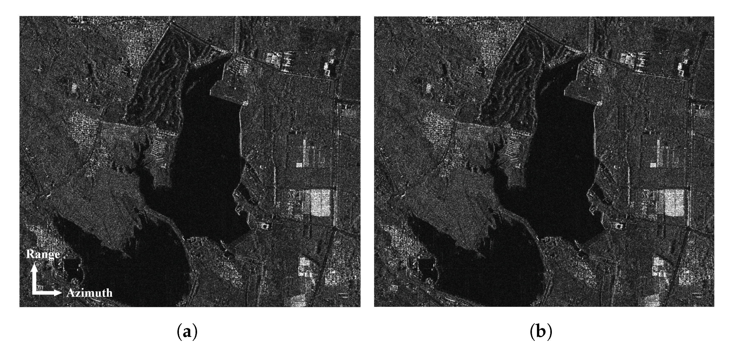
In addition, in order to more intuitively demonstrate the imaging performance of the proposed algorithm, a scene with distributed targets is simulated, in which there are point targets, the backscatter coefficients are replaced by the grayscale values of a existing SAR image, and the interval between the target points is one resolution. Figure 19 shows the imaging results that were processed by the proposed algorithm and the BP algorithm. It can be seen that the scattering characteristics of the SAR images are well displayed, and their focusing results are nearly consistent.
5. Conclusions
In this paper, a modified bistatic azimuth NLCS algorithm for the high-squint BiSAR data processing has been discussed. The algorithm is based on an accurate modified LIT spectrum that is suitable for processing high-squint BiSAR data. In the algorithm, a LRCMC operation is first performed to remove the most of the linear RCM components and mitigate the range-azimuth coupling. Subsequently, a BSRC operation is applied for compensating the residual RCM and higher order cross-coupling terms to complete the range focusing processing. Finally, by adopting higher order approximation to the azimuth FM rate and cubic phase term, a modified azimuth NLCS operation is used for eliminating the azimuth-dependence of Doppler parameters and equalizing the azimuth FM rate to accomplish azimuth compression, and the more accurate focusing results prove the effectiveness of the proposed algorithm.
Author Contributions
Conceptualization, C.L. and H.Z.; methodology, C.L.; software, C.L.; validation, C.L.; formal analysis, C.L.; investigation, C.L.; resources, Y.D.; data curation, C.L.; writing—original draft preparation, C.L.; writing—review and editing, H.Z.; visualization, C.L.; supervision, Y.D.; project administration, Y.D.; funding acquisition, H.Z. All authors have read and agreed to the published version of the manuscript.
Funding
This research was funded in part by the National Natural Science Funds for Excellent Young Scholar under Grant 61422113.
Institutional Review Board Statement
Not applicable.
Informed Consent Statement
Not applicable.
Data Availability Statement
All data generated or analyzed during this study are included in this article.
Acknowledgments
The authors would like to thank all reviewers and editors for their comments on this paper.
Conflicts of Interest
The authors declare no conflict of interest.
References
- Loffeld, O.; Nies, H.; Peters, V.; Knedlik, S. Models and useful relations for bistatic SAR processing. IEEE Trans. Geosci. Remote Sens. 2004, 10, 2031–2038. [Google Scholar] [CrossRef]
- Wang, R.; Deng, Y.; Loffeld, O.; Nies, H.; Walterscheid, I.; Espeter, T.; Klare, J.; Ender, J. Processing the Azimuth-Variant Bistatic SAR Data by Using Monostatic Imaging Algorithms Based on Two-Dimensional Principle of Stationary Phase. IEEE Trans. Geosci. Remote Sens. 2011, 10, 3504–3520. [Google Scholar] [CrossRef]
- Zhang, H.; Deng, Y.; Wang, R.; Ning, L.; Loffeld, O. Spaceborne/stationary bistatic sar imaging with terrasarx as an illuminator in staring-spotlight mode. IEEE Trans. Geosci. Remote Sens. 2016, 9, 5203–5216. [Google Scholar] [CrossRef]
- Li, C.; Zhang, H.; Deng, Y.; Wang, R.; Liu, K.; Liu, D.; Jin, G.; Zhang, Y. Focusing the L-Band Spaceborne Bistatic SAR Mission Data Using a Modified RD Algorithm. IEEE Trans. Geosci. Remote Sens. 2020, 1, 294–306. [Google Scholar] [CrossRef]
- Krieger, G.; Moreira, A. Spaceborne bi- and multistatic SAR: Potential and challenges. Proc. Inst. Elect. Eng. Radar Sonar Navig. 2006, 3, 184–198. [Google Scholar] [CrossRef] [Green Version]
- Duque, S.; Lopez-Dekker, P.; Mallorqui, J.J. Single-Pass Bistatic SAR Interferometry Using Fixed-Receiver Configurations: Theory and Experimental Validation. IEEE Trans. Geosci. Remote Sens. 2010, 6, 2740–2749. [Google Scholar] [CrossRef]
- Maslikowski, L.; Samczynski, P.; Baczyk, M.; Krysik, P.; Kulpa, K. Passive bistatic SAR imaging—Challenges and limitations. IEEE Aerosp. Electron. Syst. Mag. 2014, 7, 23–29. [Google Scholar] [CrossRef]
- Zhang, H.; Tang, J.; Wang, R.; Deng, Y.; Wang, W.; Li, N. An Accelerated Backprojection Algorithm for Monostatic and Bistatic SAR Processing. Remote Sens. 2018, 10, 140. [Google Scholar] [CrossRef] [Green Version]
- Wang, R.; Loffeld, O.; Ul-Ann, Q.; Nies, H.; Ortiz, A.M.; Samarah, A. A Bistatic Point Target Reference Spectrum for General Bistatic SAR Processing. IEEE Geosci. Remote Sens. Lett. 2008, 3, 517–521. [Google Scholar] [CrossRef]
- Wu, J.; Yang, J.; Huang, Y.; Yang, H.; Liu, Z. A point target reference spectrum for general bistatic SAR processing. In Proceedings of the IEEE International Conference on Acoustics, Speech and Signal Processing (ICASSP), Prague, Czech Republic, 22–27 May 2011; pp. 1393–1396. [Google Scholar]
- Vu, V.T.; Sjögren, T.K.; Pettersson, M.I. Two-Dimensional Spectrum for BiSAR Derivation Based on Lagrange Inversion Theorem. IEEE Geosci. Remote Sens. Lett. 2014, 7, 1210–1214. [Google Scholar] [CrossRef] [Green Version]
- Natroshvili, K.; Loffeld, O.; Nies, H.; Ortiz, A.M.; Knedlik, S. Focusing of General Bistatic SAR Configuration Data With 2-D Inverse Scaled FFT. IEEE Trans. Geosci. Remote Sens. 2006, 10, 2718–2727. [Google Scholar] [CrossRef]
- Wang, R.; Loffeld, O.; Nies, H.; Knedlik, S.; Ender, J.H.G. Chirp-scaling algorithm for bistatic SAR data in the constant-offset configuration. IEEE Trans. Geosci. Remote Sens. 2009, 47, 952–964. [Google Scholar] [CrossRef]
- Neo, Y.L.; Wong, F.; Cumming, I.G. A Two-Dimensional Spectrum for Bistatic SAR Processing Using Series Reversion. IEEE Geosci. Remote Sens. Lett. 2007, 1, 93–96. [Google Scholar] [CrossRef]
- Neo, Y.L.; Wong, F.H.; Cumming, I.G. Processing of Azimuth-Invariant Bistatic SAR Data Using the Range Doppler Algorithm. IEEE Trans. Geosci. Remote Sens. 2008, 1, 14–21. [Google Scholar] [CrossRef] [Green Version]
- Wong, F.H.; Cumming, I.G.; Neo, Y.L. Focusing bistatic SAR data using the nonlinear chirp scaling algorithm. IEEE Trans. Geosci. Remote Sens. 2008, 46, 2493–2505. [Google Scholar] [CrossRef] [Green Version]
- Qiu, X.; Hu, D.; Ding, C. An improved NLCS algorithm with capability analysis for one-stationary BiSAR. IEEE Trans. Geosci. Remote Sens. 2008, 46, 3179–3186. [Google Scholar] [CrossRef]
- Zeng, T.; Hu, C.; Wu, L.; Liu, L.; Tian, W.; Zhu, M.; Long, T. Extended NLCS algorithm of BiSAR systems with a squinted transmitter and a fixed receiver: Theory and experimental confirmation. IEEE Trans. Geosci. Remote Sens. 2013, 51, 5019–5030. [Google Scholar] [CrossRef]
- Wang, R.; Loffeld, O.; Nies, H.; Ender, J.H.G. Focusing spaceborne/airborne hybrid bistatic SAR data using wavenumber-domain algorithm. IEEE Trans. Geosci. Remote Sens. 2009, 47, 2275–2283. [Google Scholar] [CrossRef]
- Liu, B.; Wang, T.; Wu, Q.; Bao, Z. Bistatic SAR Data Focusing Using an Omega-K Algorithm Based on Method of Series Reversion. IEEE Trans. Geosci. Remote Sens. 2009, 8, 2899–2912. [Google Scholar]
- Zhang, X.; Huang, H.; Ying, W.; Wang, H.; Xiao, J. An Indirect Range-Doppler Algorithm for Multireceiver Synthetic Aperture Sonar Based on Lagrange Inversion Theorem. IEEE Trans. Geosci. Remote Sens. 2017, 6, 3572–3587. [Google Scholar] [CrossRef]
- Cumming, I.; Wong, F. Digital Processing of Synthetic Aperture Radar Data: Algorithms and Implementation; Artech House: Boston, MA, USA, 2005; pp. 113–168. [Google Scholar]
- Sun, G.; Jiang, X.; Xing, M.; Qiao, Z.; Wu, Y.; Bao, Z. Focus Improvement of Highly Squinted Data Based on Azimuth Nonlinear Scaling. IEEE Trans. Geosci. Remote Sens. 2011, 6, 2308–2322. [Google Scholar] [CrossRef]
- An, D.; Huang, X.; Jin, T.; Zhou, Z. Extended Nonlinear Chirp Scaling Algorithm for High-Resolution Highly Squint SAR Data Focusing. IEEE Trans. Geosci. Remote Sens. 2012, 9, 3595–3609. [Google Scholar] [CrossRef]
- Wang, W.; Liao, G.; Li, D.; Xu, Q. Focus Improvement of Squint Bistatic SAR Data Using Azimuth Nonlinear Chirp Scaling. IEEE Geosci. Remote Sens. Lett. 2014, 1, 229–233. [Google Scholar] [CrossRef]
- Li, D.; Liao, G.; Wang, W.; Xu, Q. Extended Azimuth Nonlinear Chirp Scaling Algorithm for Bistatic SAR Processing in High-Resolution Highly Squinted Mode. IEEE Geosci. Remote Sens. Lett. 2014, 6, 1134–1138. [Google Scholar] [CrossRef]
- Li, D.; Lin, H.; Liu, H.; Liao, G.; Tan, X. Focus Improvement for High-Resolution Highly Squinted SAR Imaging Based on 2-D Spatial-Variant Linear and Quadratic RCMs Correction and Azimuth-Dependent Doppler Equalization. IEEE Trans. Geosci. Remote Sens. 2017, 1, 168–183. [Google Scholar] [CrossRef]
- Li, Z.; Liang, Y.; Xing, M.; Huai, Y.; Zeng, L.; Bao, Z. Focusing of Highly Squinted SAR Data With Frequency Nonlinear Chirp Scaling. IEEE Geosci. Remote Sens. Lett. 2016, 1, 23–27. [Google Scholar] [CrossRef]
- Zhong, H.; Zhang, Y.; Chang, Y.; Liu, E.; Tang, X.; Zhang, J. Focus High-Resolution Highly Squint SAR Data Using Azimuth-Variant Residual RCMC and Extended Nonlinear Chirp Scaling Based on a New Circle Model. IEEE Geosci. Remote Sens. Lett. 2018, 4, 547–551. [Google Scholar] [CrossRef]
- Sun, Z.; Wu, J.; Li, Z.; Huang, Y.; Yang, J. Highly Squint SAR Data Focusing Based on Keystone Transform and Azimuth Extended Nonlinear Chirp Scaling. IEEE Geosci. Remote Sens. Lett. 2015, 1, 145–149. [Google Scholar]
- Zhao, S.; Deng, Y.; Wang, R. Attitude-steering strategy for squint spaceborne synthetic aperture radar. IEEE Geosci. Remote Sens. Lett. 2016, 8, 1163–1167. [Google Scholar] [CrossRef]
- Davidson, G.W.; Cumming, I. Signal properties of spaceborne squintmode SAR. IEEE Trans. Geosci. Remote Sens. 1997, 3, 611–617. [Google Scholar] [CrossRef] [Green Version]
- Bamler, R.; Meyer, F.; Liebhart, W. Processing of bistatic sar data from quasi-stationary configurations. IEEE Trans. Geosci. Remote Sens. 2007, 11, 3350–3358. [Google Scholar] [CrossRef]
- Yeo, T.S.; Tan, N.L.; Zhang, C.B.; Lu, Y.H. A new subaperture approach to high squint SAR processing. IEEE Trans. Geosci. Remote Sens. 2001, 5, 954–968. [Google Scholar]
- Jin, M.Y.; Wu, C. A SAR correlation algorithm which accommodates large-range migration. IEEE Trans. Geosci. Remote Sens. 1984, 6, 592–597. [Google Scholar] [CrossRef]
- Zhang, S.; Xing, M.; Xia, X.; Zhang, L.; Guo, R.; Bao, Z. Focus Improvement of High-Squint SAR Based on Azimuth Dependence of Quadratic Range Cell Migration Correction. IEEE Geosci. Remote Sens. Lett. 2013, 1, 150–154. [Google Scholar] [CrossRef]
- An, D.; Li, Y.; Huang, X.; Li, X.; Zhou, Z. Performance evaluation of frequency-domain algorithms for chirped low frequency uwb sar data processing. IEEE J. Sel. Top. Appl. Earth Obs. Remote Sens. 2014, 2, 678–690. [Google Scholar] [CrossRef]
- Davidson, G.W.; Cumming, I.G. A chirp scaling approach for processing squint mode SAR data. Aerosp. Electron. Syst. IEEE Trans. 1996, 32, 121–133. [Google Scholar] [CrossRef]
- Krieger, G.; Fiedler, H.; Houman, D.; Moreira, A. Analysis of system concepts for bi-and multi-static sar missions. In Proceedings of the IEEE International Geoscience and Remote Sensing Symposium, Toulouse, France, 21–25 July 2003; Volume 2, pp. 770–772. [Google Scholar]
- Walterscheid, I.; Brenner, A.; Ender, J. Results on bistatic synthetic aperture radar. Electron. Lett. 2004, 19, 1224–1225. [Google Scholar] [CrossRef] [Green Version]
Figure 1.
Geometry of general bistatic configuration.

Figure 2.
The slant range errors that are induced by the different approximations. (a) The third-order approximation and (b) formula (7).
Figure 2.
The slant range errors that are induced by the different approximations. (a) The third-order approximation and (b) formula (7).

Figure 3.
Spectrum of simulated high-squint BiSAR data. (a) Before and (b) after LRCMC operation.

Figure 4.
Block diagram of the proposed modified bistatic azimuth NLCS algorithm.

Figure 5.
An illustration of linear RCMC. (a) Bistatic SAR imaging geometry. (b) Data before LRCMC and after LRCMC. We can see that the target points T0, T3, T4 with different RCM trajectories are at the same range gate after the LRCMC operation. At this time, the traditional RD and CS algorithm will no longer be applicable.
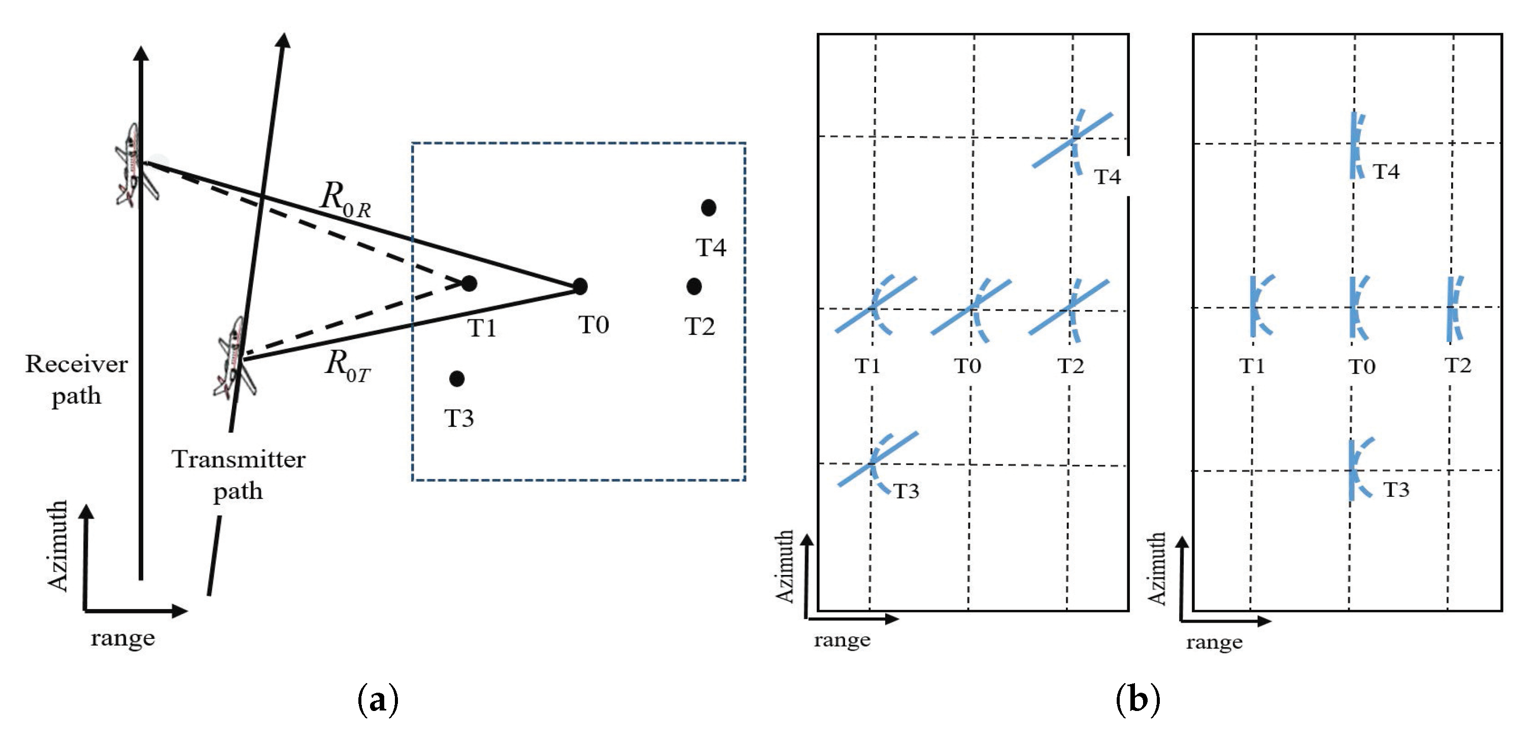
Figure 6.
Diagram for the residual RCM evaluation. (a) Diagram of the residual RCMs of targets T0–T4. (b) A diagram of the residual RCMs between targets T1, T2, and target T0, respectively. It can be seen, from (b), that the residual RCM is very weakly range dependent, so we can use the RCM at the reference range to compensate.
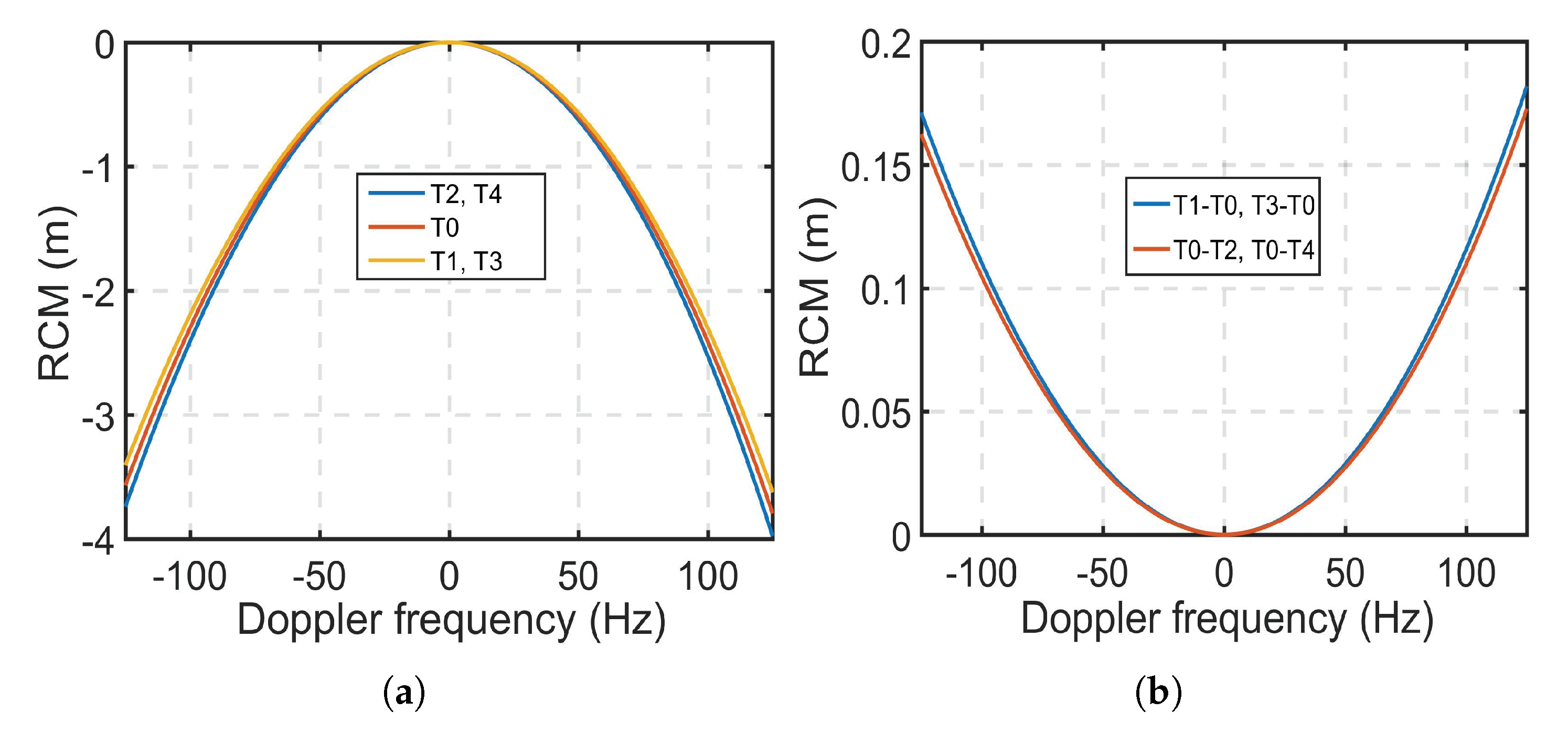
Figure 7.
Diagrams for the azimuth FM rate approximation evaluations. (a) Azimuth FM rates for different order approximations. (b) Relationships between the QPE induced by the approximated azimuth FM rate versus azimuth position.
Figure 7.
Diagrams for the azimuth FM rate approximation evaluations. (a) Azimuth FM rates for different order approximations. (b) Relationships between the QPE induced by the approximated azimuth FM rate versus azimuth position.
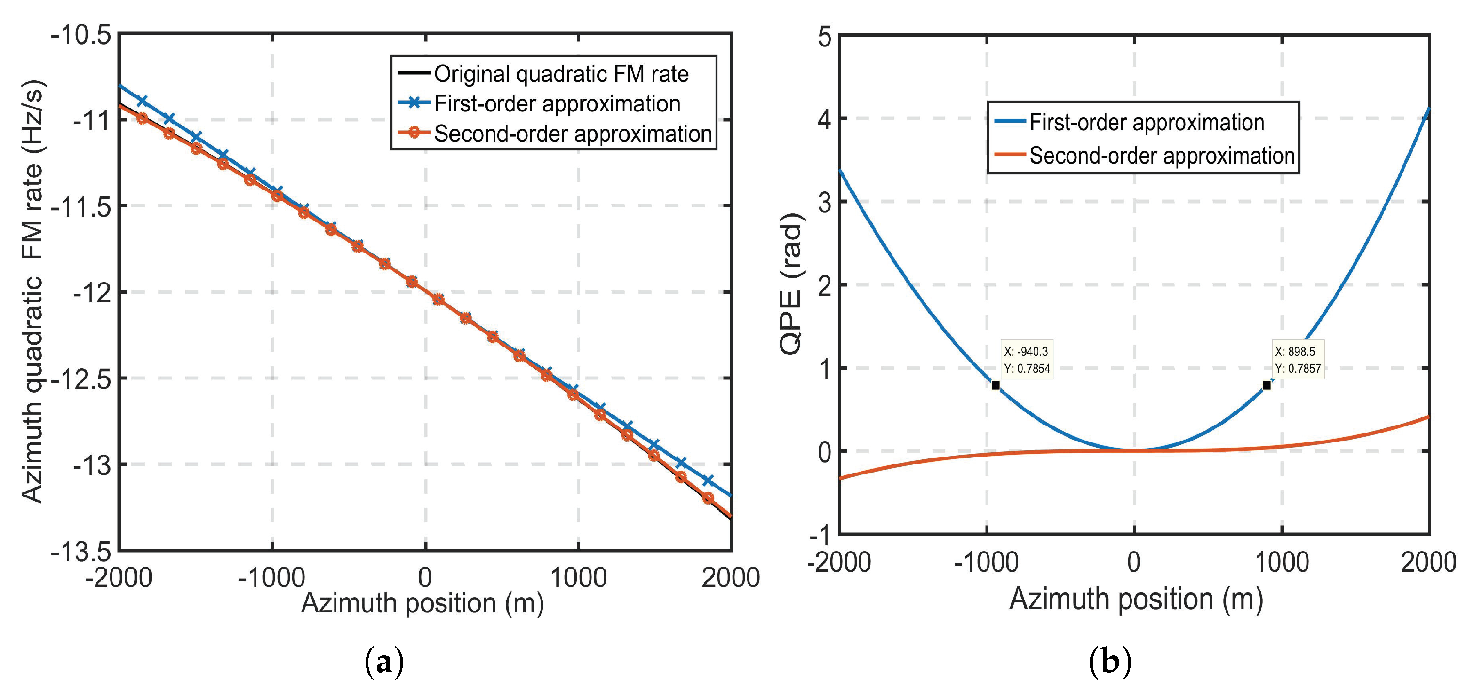
Figure 8.
Diagrams for the azimuth-dependent cubic phase term evaluation.
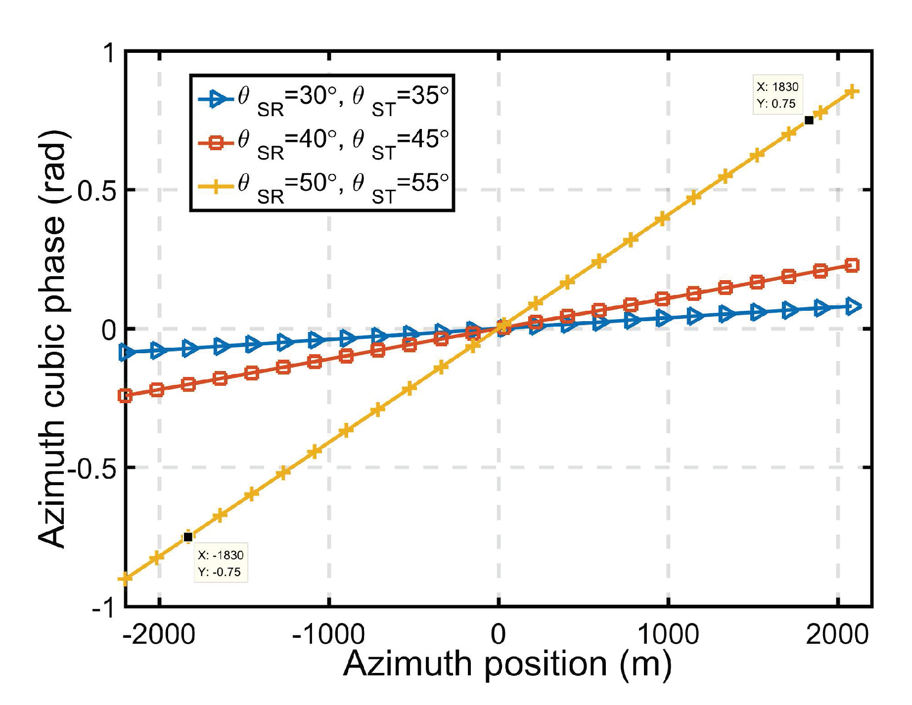
Figure 9.
Diagrams for the azimuth NLCS operation. (a) The quadratic phase curves of different targets before azimuth NLCS. (b)After azimuth NLCS.
Figure 9.
Diagrams for the azimuth NLCS operation. (a) The quadratic phase curves of different targets before azimuth NLCS. (b)After azimuth NLCS.
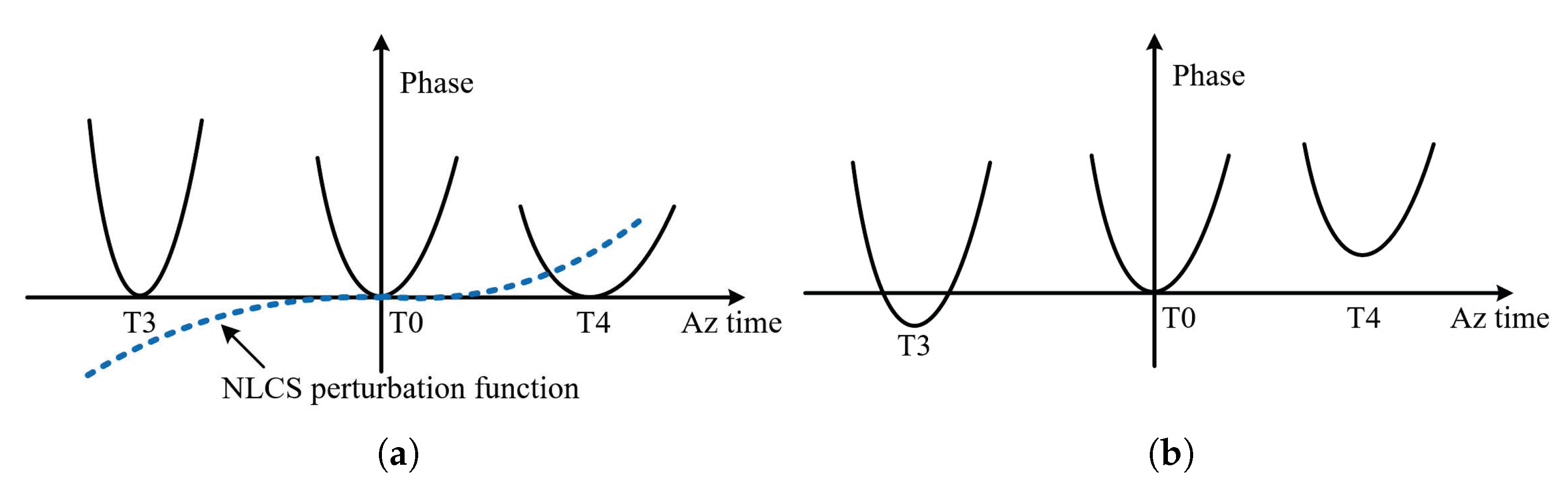
Figure 10.
Flight geometry and target layout for the simulation.
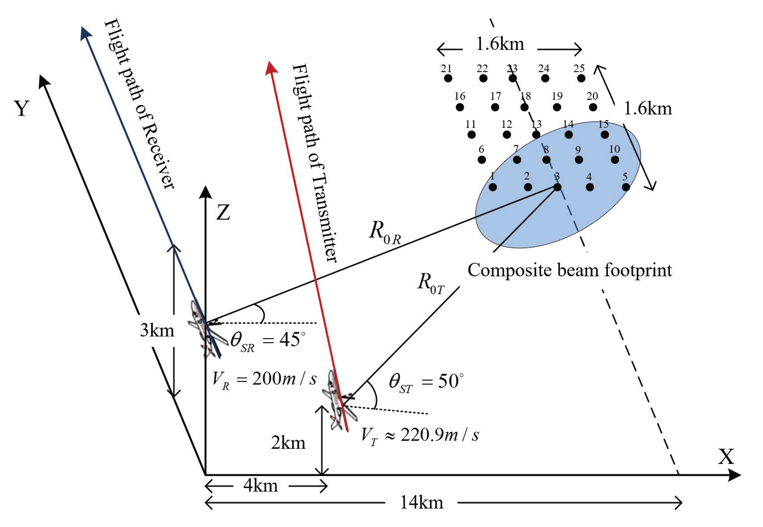
Figure 11.
(a) The echo data of the 25 point targets. (b) The RCM trajectories in 2-D time domain after range compression and (c) LRCMC operation. (d) The RCM trajectories in the range Doppler domain before the BSRC operation. (e) And after the BSRC operation. (f) The phase curves of the targets 5, 13, and 21 in 2-D time domain before the proposed modified azimuth NLCS operation. (g) And after the proposed NLCS operation. (h) The RCM trajectories in 2-D time domain after the above processing steps.

Figure 12.
Twenty-five simulated point targets, which are processed by using the proposed modified bistatic azimuth NLCS algorithm.
Figure 12.
Twenty-five simulated point targets, which are processed by using the proposed modified bistatic azimuth NLCS algorithm.
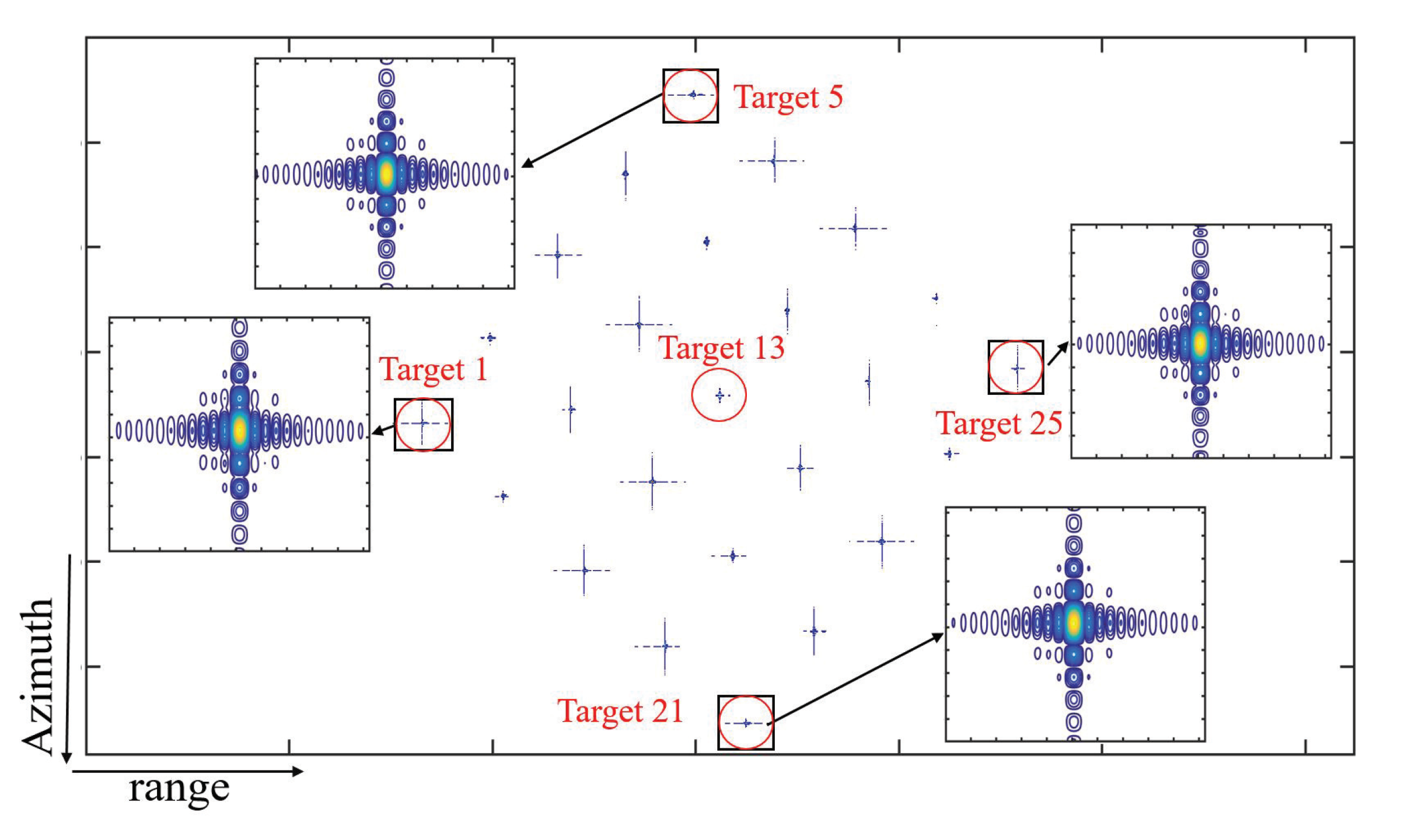
Figure 13.
(a) Contour plot of target 13 focused by the proposed algorithm. (b) Range impulse responses of target 13 obtained by the proposed algorithm (blue line) and BP algorithm (red line). (c) Azimuth impulse responses of target 13.
Figure 13.
(a) Contour plot of target 13 focused by the proposed algorithm. (b) Range impulse responses of target 13 obtained by the proposed algorithm (blue line) and BP algorithm (red line). (c) Azimuth impulse responses of target 13.
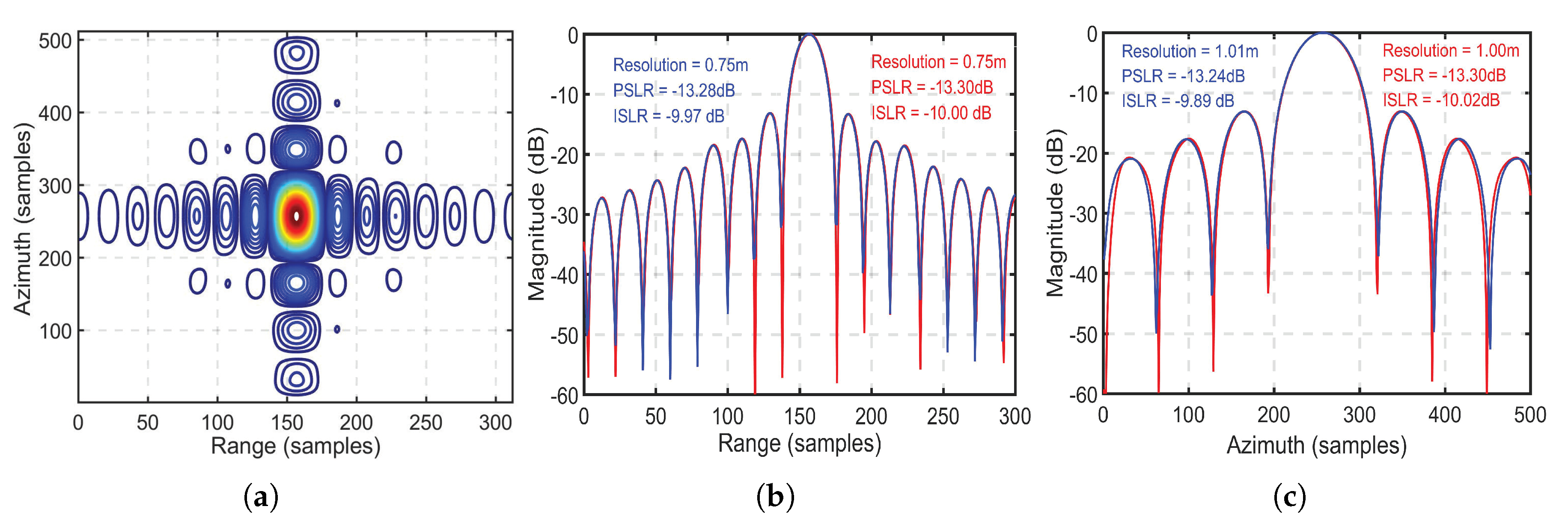
Figure 14.
(a) Contour plot of target 13 focused by the proposed algorithm. (b) Range impulse responses of target 25 obtained by the proposed algorithm (blue line) and BP algorithm (red line). (c) Azimuth impulse responses of target 25.
Figure 14.
(a) Contour plot of target 13 focused by the proposed algorithm. (b) Range impulse responses of target 25 obtained by the proposed algorithm (blue line) and BP algorithm (red line). (c) Azimuth impulse responses of target 25.
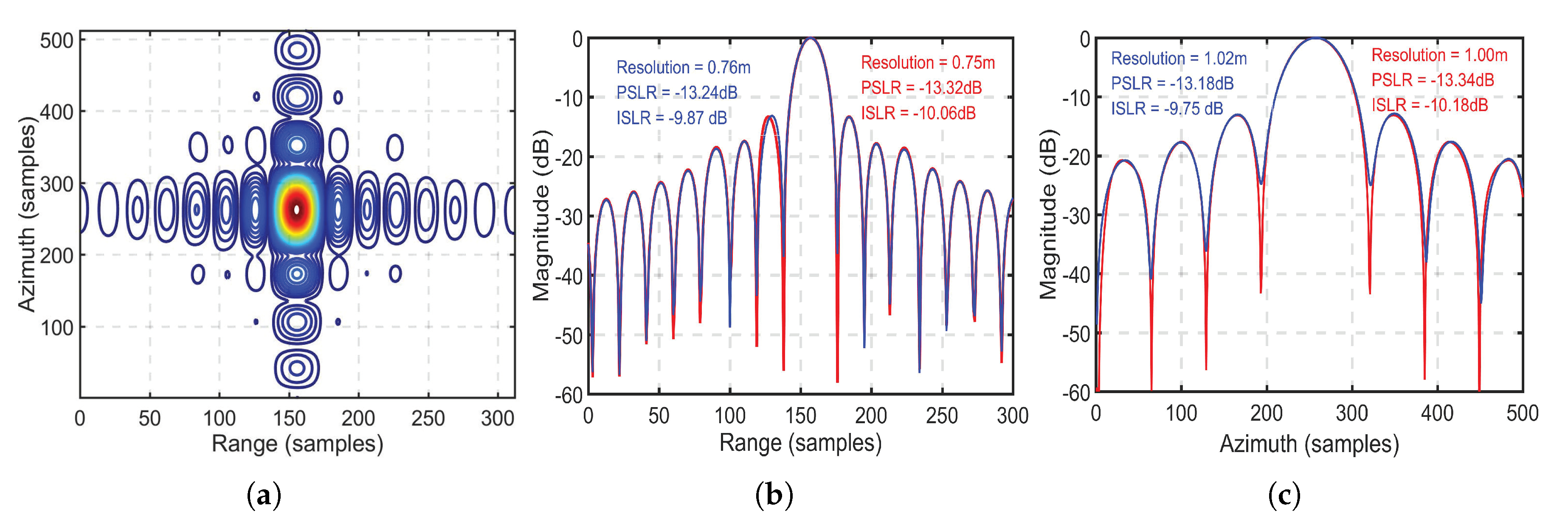
Figure 15.
Simulation results of target 14 using different algorithms. (a) The aforementioned modified Zhang’s RDA. (b) Wong’s NLCS algorithm. (c) Proposed algorithm.
Figure 15.
Simulation results of target 14 using different algorithms. (a) The aforementioned modified Zhang’s RDA. (b) Wong’s NLCS algorithm. (c) Proposed algorithm.
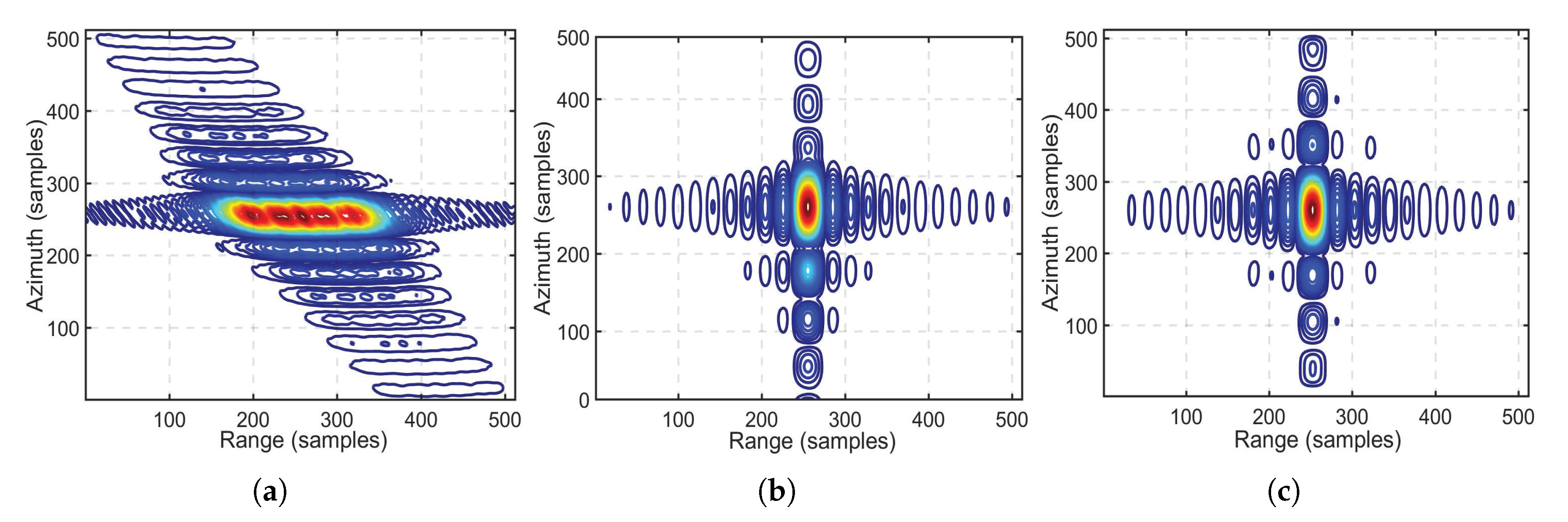
Figure 16.
Simulation results of target 15 processed using different algorithms. (a) The aforementioned modified Zhang’s RDA. (b) Wong’s NLCS algorithm. (c) Proposed algorithm.
Figure 16.
Simulation results of target 15 processed using different algorithms. (a) The aforementioned modified Zhang’s RDA. (b) Wong’s NLCS algorithm. (c) Proposed algorithm.
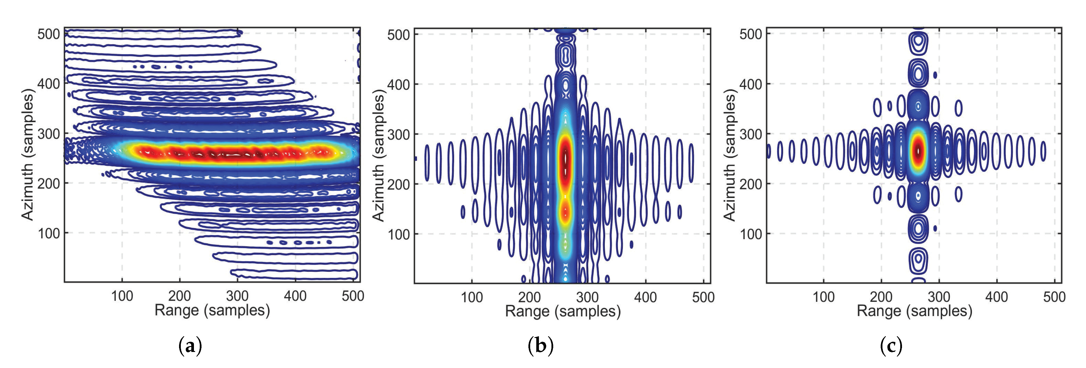
Figure 17.
Simulation results of target 18 processed using different algorithms. (a) The aforementioned modified Zhang’s RDA. (b) Wong’s NLCS algorithm. (c) Proposed algorithm.
Figure 17.
Simulation results of target 18 processed using different algorithms. (a) The aforementioned modified Zhang’s RDA. (b) Wong’s NLCS algorithm. (c) Proposed algorithm.
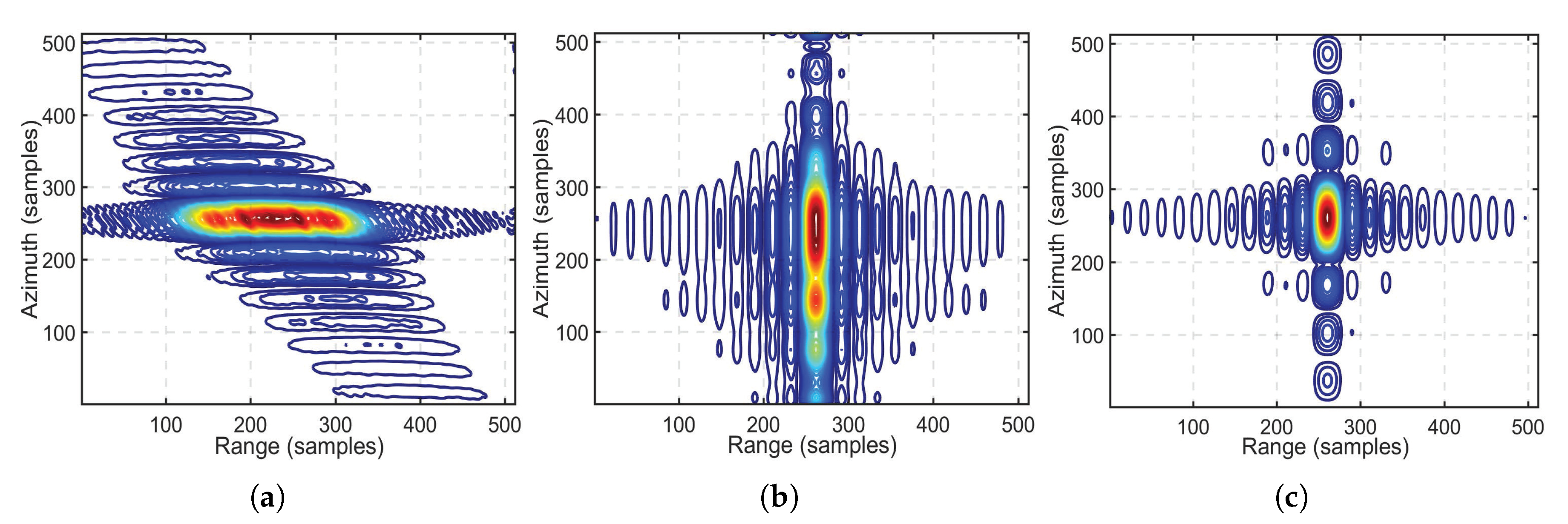
Figure 18.
Simulation results of target 23 processed using different algorithms. (a) The aforementioned modified Zhang’s RDA. (b) Wong’s NLCS algorithm. (c) Proposed algorithm.
Figure 18.
Simulation results of target 23 processed using different algorithms. (a) The aforementioned modified Zhang’s RDA. (b) Wong’s NLCS algorithm. (c) Proposed algorithm.

Figure 19.
Imaging results of scene simulation processed by the different algorithms. (a) The proposed algorithm. (b) The BP algorithm.
Figure 19.
Imaging results of scene simulation processed by the different algorithms. (a) The proposed algorithm. (b) The BP algorithm.

Table 1.
BiSAR System Simulation Parameters.
| Simulation Parameters | Receiver | Transmitter |
|---|---|---|
| Velocity in y-direction | 200 m/s | 200 m/s |
| Velocity in x-direction | 0 m/s | 20 m/s |
| Altitude | 3000 m | 2000 m |
| Squint angle | 45 | 50 |
| Center frequency | 9.6 GHz | |
| Range bandwidth | 200 MHz | |
| Transmitted pulse duration | 20 s | |
| PRF | 500 | |
| Antenna length | 2 m | |
Table 2.
Measured Results of the Selected Targets.
| Range | Azimuth | ||||||
|---|---|---|---|---|---|---|---|
| Target | Resolution (m) | PSLR (dB) | ISLR (dB) | Resolution (m) | PSLR (dB) | ISLR (dB) | |
| Zhang’s RDA | 14 | 0.885 | −17.33 | −3.58 | 1.94 | −7.30 | −3.08 |
| 15 | 0.815 | −15.68 | −4.66 | 2.11 | −6.54 | −1.19 | |
| 18 | 0.796 | −14.21 | −8.92 | 1.53 | −10.89 | −8.18 | |
| 23 | 0.782 | −14.93 | −7.04 | 1.66 | −9.33 | −6.73 | |
| Wong’s NLCSA | 14 | 0.759 | −12.87 | −10.80 | 1.12 | −12.01 | −8.23 |
| 15 | 0.754 | −12.05 | −9.13 | 1.24 | −10.41 | −5.31 | |
| 18 | 0.760 | −12.58 | −9.76 | 1.47 | −12.86 | −5.37 | |
| 23 | 0.754 | −11.33 | −9.09 | 1.53 | −9.91 | −4.56 | |
| Proposed method | 14 | 0.757 | −13.39 | −10.30 | 1.01 | −13.26 | −10.13 |
| 15 | 0.752 | −13.48 | −10.44 | 1.02 | −13.18 | −10.25 | |
| 18 | 0.751 | −13.21 | −9.81 | 1.01 | −13.23 | −10.30 | |
| 23 | 0.758 | −13.01 | −9.64 | 1.02 | −13.11 | −10.33 | |
Publisher’s Note: MDPI stays neutral with regard to jurisdictional claims in published maps and institutional affiliations. |
© 2021 by the authors. Licensee MDPI, Basel, Switzerland. This article is an open access article distributed under the terms and conditions of the Creative Commons Attribution (CC BY) license (https://creativecommons.org/licenses/by/4.0/).
Share and Cite
MDPI and ACS Style
Li, C.; Zhang, H.; Deng, Y. Focus Improvement of Airborne High-Squint Bistatic SAR Data Using Modified Azimuth NLCS Algorithm Based on Lagrange Inversion Theorem. Remote Sens. 2021, 13, 1916. https://doi.org/10.3390/rs13101916
AMA Style
Li C, Zhang H, Deng Y. Focus Improvement of Airborne High-Squint Bistatic SAR Data Using Modified Azimuth NLCS Algorithm Based on Lagrange Inversion Theorem. Remote Sensing. 2021; 13(10):1916. https://doi.org/10.3390/rs13101916
Chicago/Turabian StyleLi, Chuang, Heng Zhang, and Yunkai Deng. 2021. "Focus Improvement of Airborne High-Squint Bistatic SAR Data Using Modified Azimuth NLCS Algorithm Based on Lagrange Inversion Theorem" Remote Sensing 13, no. 10: 1916. https://doi.org/10.3390/rs13101916
Note that from the first issue of 2016, this journal uses article numbers instead of page numbers. See further details here.