
Phenological Changes of Mongolian Oak Depending on the Micro-Climate Changes Due to Urbanization


1
Graduate School of Seoul Women’s University, Seoul Women’s University, 621 Hwarang-no, Nowon-gu, Seoul 01797, Korea
2
Division of Ecological Survey Research, National Institute of Ecology, 1210 Geumgang-no, Maseo-myeon, Seocheon 33657, Korea
3
Division of Chemistry and Bio-Environmental Sciences, Seoul Women’s University, 621 Hwarang-no, Nowon-gu, Seoul 01797, Korea
*
Author to whom correspondence should be addressed.
Remote Sens. 2021, 13(10), 1890; https://doi.org/10.3390/rs13101890
Submission received: 5 April 2021
/
Revised: 8 May 2021
/
Accepted: 10 May 2021
/
Published: 12 May 2021
(This article belongs to the Special Issue Remote Sensing of Land Surface Phenology)
Abstract
:Urbanization and the resulting increase in development areas and populations cause micro-climate changes such as the urban heat island (UHI) effect. This micro-climate change can affect vegetation phenology. It can advance leaf unfolding and flowering and delay the timing of fallen leaves. This study was carried out to clarify the impact of urbanization on the leaf unfolding of Mongolian oak. The survey sites for this study were established in the urban center (Mts. Nam, Mido, and Umyeon in Seoul), suburbs (Mts. Cheonggye and Buram in Seoul), a rural area (Gwangneung, Mt. Sori in Gyeonggi-do), and a natural area (Mt. Jeombong in Gangwon-do). Green-up dates derived from the analyses of digital camera images and MODIS satellite images were the earliest in the urban center and delayed through the suburbs and rural area to the natural area. The difference in the observed green-up date compared to the expected one, which was determined by regarding the Mt. Jeombong site located in the natural area as the reference site, was the biggest in the urban center and decreased through the suburbs and rural area to the natural area. Green-up dates in the rural area, suburbs, and urban center were earlier by 11.0, 14.5, and 16.3 days than the expected ones. If these results are transformed into the air temperature based on previous research results, it could be deduced that the air temperature in the urban center, suburbs, and rural area rose by 3.8 to 4.6 °C, 3.3 to 4.1 °C, and 2.5 to 3.1 °C, respectively. Green-up dates derived based on the accumulated growing degree days (AGDD) showed the same trend as those derived from the image interpretation. Green-up dates derived from the change in sap flow as a physiological response of the plant showed a difference within one day from the green-up dates derived from digital camera and MODIS satellite image analyses. The change trajectory of the curvature K value derived from the sap flow also showed a very similar trend to that of the curvature K value derived from the vegetation phenology. From these results, we confirm the availability of AGDD and sap flow as tools predicting changes in ecosystems due to climate change including phenology. Meanwhile, the green-up dates in survey sites were advanced in proportion to the land use intensity of each survey site. Green-up dates derived based on AGDD were also negatively correlated with the land use intensity of the survey site. This result implies that differences in green-up dates among the survey sites and between the expected and observed green-up dates in the urban center, suburbs, and rural area were due to the increased temperature due to land use in the survey sites. Based on these results, we propose conservation and restoration of nature as measures to reduce the impact of climate change.
1. Introduction
Urbanization is one of the major social and scientific changes spreading around the world [1,2]. It significantly alters land surface conditions and has profound impacts on terrestrial ecosystem processes and services [3,4,5,6,7]. Changes in land use release greenhouse gases into the atmosphere by changing the patterns of carbon storage and accelerate climate change by breaking the balance of the carbon budget [2]. An increase in atmospheric CO2 due to intensive use of land and fossil fuel destroys the balance of the global carbon cycle maintained in an equilibrium fashion [2,8,9,10,11]. In addition, increased development areas and populations cause changes in weather factors and affect terrestrial ecosystems [3,4,5,6,12]. Inadvertent weather factor changes in urban areas form an important effect on regional climate change [13,14,15,16].
Urbanization is an important anthropogenic influence on climate and has significantly affected terrestrial ecosystems [12,17]. It can modify local climate on daily, seasonal, and annual scales [18] and increase extreme climate events [19,20,21,22]. Changes in climate resulting from urbanization, therefore, can be considered a type of climate change on a local scale [23]. Such a change in local climate in an urban area is referred to as the “urban heat island (UHI) effect”. The UHI effect is characterized by elevated temperatures in urban areas, compared to the surrounding rural areas [7,24,25]. It can affect regional climate change, increase environmental pollution, elevate energy and water consumption, affect the development of meteorological events such as increased precipitation, and have a significant impact on human health [16,26,27].
In phenological research, urban areas are important areas for study because they enable an assessment of the potential future effects of climate change on plant development [17,28]. Increased temperature by UHI can affect vegetation phenology such as the start of the season (SOS) and the end of the growing season (EOS) [25,29,30,31]. It is very important to understand the impact of UHI on phenology because the intensity of the UHI effect is similar to the expected temperature change in the near future [7].
Current climate change has a strong impact on vegetation phenology [6,32,33,34,35,36,37], and it causes changes in the timing of plant developmental phases, affecting the carbon budget of the terrestrial ecosystem [38,39,40,41]. Phenological characteristics are closely related to variation in weather factors [6,42,43,44,45], many of which can affect vegetation phenology such as green-up, budburst, and leaf senescence [17].
Among the numerous techniques to observe phenology, using digital camera and MODIS satellite images requires less time and cost to collect data [46,47]. Time-lapse photography provides very exact temporal sampling at daily intervals for assessing phenology. Satellite remote sensing provides decades of records of vegetation phenology across larger spatial scales than other technologies [48]. Remote sensing also has the advantage of providing large temporal records of vegetation phenology over larger spatial scales than other techniques [17,48]. In particular, the method using both digital camera and MODIS satellite images has sufficient spatial resolution to obtain detailed information about vegetation and land cover types and can collect data with more flexible spatial resolution, thereby resolving the problems pointed out in the existing data collection [17,26,46,49].
Recently, beyond the level of checking phenological phases by observing the external forms of plants, a study method to confirm the plant phenological phases through physiological responses such as sap flow time series estimates was also proposed [17,50]. Water availability is regulated by the timing and periodicity of leaf production and is very important for plant growth [51,52]. According to many studies investigating the relationship between phenology and sap flow, sap flow is closely related to the change in leaf area [50,53,54], since plants draw water from the xylem by tension from the leaves during the transpiration period [55], and the amount of transpiration increases depending on the formation of leaves. Therefore, sap flow usually has a linear relationship with leaf area development [17,50,54]. Phenological events emerging through appearance may be difficult to observe accurately and precisely due to various influences [56,57], and the method of color wavelength analysis of the leaves applies well for deciduous plants, but there will be limitations to evergreen plants. In this respect, a method of monitoring physiological changes according to seasonal changes may be more versatile [58]. In addition, since the phenophase using instrumental techniques can be better specified than pure observations and qualified guesses, the onset of spring phenological stages such as leaf area development can be easily identified from sap flow measurements [50]. Ecophysiological measurements such as sap flow measurement can provide additional value in the objectification of phenological studies [50]. Therefore, sap flow has been widely utilized as a tool to diagnose the development of the phenological phases of plants [30,51,54,59].
The objectives of this study are to (1) find the phenological trajectory of vegetation through analysis of MODIS satellite and digital camera images, (2) investigate how micro-climate change caused by urbanization affects vegetation phenology, (3) diagnose the phenological trajectory of vegetation through the physiological response of plants, and (4) prepare an ecosystem management strategy to adapt to climate change.
2. Materials and Methods
2.1. Study Area
To find out the response of phenological events according to the climatic condition, we selected three areas different in land use intensity, such as urban, rural, and natural areas on the same latitude. The phenological signal is evident in deciduous broad-leaved forests because the changes in the canopy are large depending on the stage of the phenology [60]. In this study, therefore, we selected the target species as Quercus mongolica Fisch. ex Ledeb., a dominant species in the deciduous broad-leaved forest of Korea. Since the Q. mongolica that belongs to the Quercus genus grows at the highest elevation in South Korea, it is considered to be sensitive to temperature rises due to climate change. Seven sites including Mts. Nam, Mido, and Umyeon in the urban center, Mts. Cheonggye and Buram in the suburbs, Gwangneung (Mt. Sori) in a rural area, and Mt. Jeombong in a natural area were selected for analysis (Figure 1, Table 1). The urbanization ratio was calculated from the ratio of development area to the total area within a 5 km radius from the study area by a geographic interpolation system (GIS) using the national land use map (National Geographic Information Institute, 2016). The urbanization rates of Mts. Nam, Mido, Umyeon, Cheonggye, Buram, and Sori (Gwandneung) were 76.07, 70.35, 52.44, 35.80, 49.60, and 6.38, respectively, and Mt. Jeombong was not urbanized at all as it is located in a natural area (Table 2).
2.2. Digital Camera and Satellite Image Acquisition
We installed digital cameras (Model Ltl-6210M, Little Acorn Outdoors, Denmark, WI, USA) near the top of each tower or tree, looking north and angled slightly downward, providing a view across the canopy. To acquire daily photos, each camera was set to record JPEG images three times per day (09:00, 12:30, and 14:30). In order to maintain consistency, only 12:30 images were used for the analysis (Table 3).
As the notion the shorter the collection cycle, the higher the clarity applies [61], we used MODIS (MODerate-Resolution Imaging Spectroradiometer) 500m resolution land surface imagery (MOD09GA), which is supplied at daily intervals as multi-spectral satellite images. The MODIS satellite is a payload scientific instrument placed in the earth’s orbit by NASA in December 1999 on the Terra (EOS AM) satellite. The MODIS satellite imagery measures the surface temperature of the land and ocean, and the distribution map of the earth’s vegetation is re-synthesized with control variables such as clouds and distributed free of charge by NASA. The MODIS satellite is suitable for monitoring phenological changes because the sensor incorporates enhanced cloud detection, atmospheric correction, georeferencing, and the ability to monitor vegetation [39,62].
2.3. Digital Camera Image Analysis
An annual vegetation phenological cycle inferred from remote sensing is characterized by four stages that define the key phenological phases at annual time scales: (1) green-up, (2) maturity, (3) senescence, and (4) dormancy [17,60,63]. Phenological signals remain low values during the dormancy phase and then increase rapidly as the green-up phase begins. When the leaves reach maturity, signals no longer increase but maintain a high value. After that, the plants enter into the senescence phase, and the signals decrease radically. As the dormancy phase begins, the phenological signals return to the lowest value of the initial phase. As such, an inflection point at which the curvature rapidly changes in the phenological signal curve may be interpreted as the start date of each stage [17,63]. The formula for obtaining the curvature K value of the inflection point is as follows:
where t is time, c is the amplitude of an increase or decrease in the green value, d is the baseline value of the dormant season, and a and b control the lower and upper limits of the function [17,64,65,66].
To extract phenological signals, we collected images from the digital cameras periodically and classified them into red, green, and blue bands. Using digital numbers for each band, we calculated the average excess green index (ExG) for each ROI based on the equation [64,65]
where ρRED, ρGREEN, and ρBLUE are values in red, green, and blue channels acquired from digital camera images, respectively. The region of interest (ROI) is used when digital camera images are analyzed to clarify phenological changes [67]. As the digital camera images include a mixture of the sky, landscape, and other factors, the ROI is limited to the crown layer to extract the phenological signal from the images. Furthermore, because, in these study sties, the Q. mongolica stands are mixed with Quercus variabilis Blume and Quercus serrata Murray stands, and other species, the ROI was limited to pure stands of Q. mongolica, and we tried to avoid mountains and sky [60,64] (Figure 2). In this study, we set up a number of ROIs for the images of the Q. mongolica community in each site and extracted the ExG index.
ExG = 2 × ρGREEN − (ρRED + ρBLUE)
2.4. Analysis of Satellite Images
The MOD09GA datasets are comprised of seven bands, including visible light bands and near-infrared bands. The EVI in MODIS was calculated using red (Band 1: 620–670 µm), green (Band 4: 545–565 µm), blue (Band 3: 459–479 µm), and near-infrared (Band 2: 841–876 µm) based on the equations. The vegetation index uses the EVI index, which is an improvement over other indexes. The EVI index is an improved vegetation index to reduce the effects of spatial differences by using blue bands in areas with large spatial differences and is suitable for observing seasonal changes in vegetation by reflecting the characteristics of the canopy [62]. The EVI calculations used in the analysis are as follows:
where ρnir, ρred, and ρblue are values in near-infrared, red, and blue bands. MODIS satellite images were reprojected to TM (transverse Mercator) coordinates because they use a sinusoidal projection. Based on the extracted data, the EVI index for each study site was derived. Then, the EVI was obtained using the smooth curve fitting method to remove variation and to gather trends because interpretation error can occur due to data errors and variation depending on weather conditions [17]. In this study, the EVI was smoothed to the 80th percentile using an exponentially weighted moving average (EWMA). The EWMA was defined as
where t is the day of year (DoY); St is the EWMA value at the DoY; Yt is the EVI value at the DoY; and α is the smoothing coefficient.
EVI = 2.5 × (ρnir − ρred)/{ρnir + (6 × ρred − 7.5 × ρblue) + 1}
St = α × Yt + (1 − α) × St−1 (t > 1, S1 = Y1)
2.5. Sap Flow Measurement
To analyze the relationship between the phenological signal and the physiological responses of plants, we collected data from a sap flow measurement instrument (model SFM1 Sap Flow Meter, ICT international, Armidale, Australia) installed in the study sites. Measured individuals were randomly selected from individuals included in the ROI. Sap flow velocity (cm3∙hr−1) was calculated by heat pulse, and temperature was measured from the thermistor inserted 7.5 mm and 22.5 mm inside the removed bark [68]. The seasonal trajectory of sap flow was interpreted using curvature K (formula 2) based on the daily sap velocity. The transition date of the sap flow was compared with the phenological transition date obtained from the digital camera and MODIS installed at the same site.
2.6. Data Correction
The green-up date of Q. mongolica derived from digital camera and MODIS satellite images showed a difference depending on the study site. According to [69], increases in latitude of 1° N, longitude of 1° E, and altitude of 100 m result in delays of 2.6 ± 0.2 days, 0.6 ± 0.1 days, and 2.1 ± 0.2 days, respectively, in the leaf unfolding date. Based on this information, we corrected the difference in leaf unfolding dates due to differences in latitude, longitude, and altitude among the study areas.
On the other hand, we designated the Mt. Jeombong site as the reference site to clarify the effect of urbanization. Mt. Jeombong maintains a healthy and integrated stand of Q. mongolica as it is designated as a reserve by the Korea Forest Service and thereby escapes artificial interferences. Based on the Mt. Jeombong data, the expected dates of green-up were obtained by reflecting the geographic and topographic location of each study site. The effect of urbanization on plant phenology in each study area was determined by comparing the differences between the expected and observed dates of green-up in each site.
2.7. Weather Factor Collection and Analysis
To analyze the correlation between phenological events and weather factors and identify the weather conditions at the time of major phenological phases, the atmospheric temperature measurement instrument HOBO (HOBO Pro v2 Temp/RH Temp, Onset Computer, Bourne, MA, USA) was installed. The temperature was measured every 30 minutes every day, and the data measured at 12:30 were used due to compatibility with the digital camera.
Based on the collected weather data, AGDD (accumulated growing degree days) were calculated to analyze the temperature threshold of the plant’s green-up period. The formula for calculating AGDD is as follows:
where Tmax and Tmin are the maximum and minimum air temperatures, respectively, and TΔ is the temperature below which plant growth is zero. In this study, we assumed a minimum temperature threshold of 5 °C for enzymatic activity in Q. mongolica based on studies of [70,71].
3. Results
3.1. The Green-up Date of Mongolian Oak
ExG values obtained from digital cameras clearly indicate the phenological changes of Mongolian oak (Figure 3). The green-up date of Mongolian oak, derived from the curvature K value of the digital camera ExG, was the earliest in the urban area and gradually delayed moving through the suburban and rural areas toward the natural area with 94, 95, 95, 95, 97, 102, and 117 days in Mts. Nam, Mido, Umyeon, Buram, Cheonggye, Sori (Gwangneung), and Jeombong, respectively, based on the day of year (DoY) (Table 4).
EVI values obtained from MODIS images also clearly indicate the phenological changes of Mongolian oak (Figure 4). The green-up date of Mongolian oak, derived from the curvature K value of the MODIS image EVI, showed a similar trend to the result from the digital camera, with 94, 96, 97, 95, 96, 104, and 114 days in Mts. Nam, Mido, Umyeon, Buram, Cheonggye, Sori (Gwangneung), and Jeombong, respectively, based on the DoY (Table 4).
In addition, to clarify the differences among sites due to artificial interference, the expected dates of green-up were obtained through latitude, altitude, and elevation correction based on the natural area, Mt. Jeombong. This was compared with the actual observed dates of the study site (Table 4). The green-up date observed from the ExG of Mt. Nam was DoY 94, which is 16 days earlier than the expected DoY 110. The green-up date observed from the ExG of Mt. Mido was DoY 95, which is 18 days earlier than the expected DoY 113. The green-up date observed from the ExG of Mt. Umyeon was DoY 95, which is 15 days earlier than the expected DoY 110. The green-up date observed from the ExG of Mt. Cheonggye was DoY 97, which is 14 days earlier than the expected DoY 111. The green-up date observed from the ExG of Mt. Buram was DoY 95, which is 15 days earlier than the expected DoY 110. The green-up date observed from the ExG of Gwangneung (Mt. Sori) was DoY 103, which is 11 days earlier than the expected DoY 114 (Table 4).
The green-up date observed from the EVI of Mt. Nam was DoY 94, which is 16 days earlier than the expected DoY 110. The green-up date observed from the EVI of Mt. Mido was DoY 96, which is 18 days earlier than the expected DoY 114. The green-up date observed from the EVI of Mt. Umyeon was DoY 97, which is 15 days earlier than the expected DoY 112. The green-up date observed from the EVI of Mt. Cheonggye was DoY 96, which is 14 days earlier than the expected DoY 110. The green-up date observed from the EVI of Mt. Buram was DoY 96, which is 15 days earlier than the expected DoY 111. The green-up date observed from the EVI of Gwangneung (Mt. Sori) was DoY 104, which is 11 days earlier than the expected DoY 115 (Table 4).
As a result of analysis, the correlation between green-up dates derived from ExG and EVI values and land use intensity showed a significant negative correlation (Figure 5).
3.2. Accumulated Growing Degree Days (AGDD)
Green-up dates estimated by AGDD in each study site are shown in Table 5. Green-up dates expressed as DoY were 94, 95, 95, 97, 96, 103, and 114 in Mts. Nam, Mido, Woomyeon, Cheonggye, Buram, Sori (Gwangneung), and Jeombong, respectively (Table 5). AGDD for green-up dates derived from the ExG of the digital camera were 160.3 °C, 158.2 °C, 156.3 °C, 162.2 °C, 162.3 °C, 156.6 °C, and 160.5 °C, and AGDD for green-up dates derived from the EVI of MODIS images were 160.3 °C, 166.9 °C, 162.6 °C, 153.2 °C, 168.3 °C, 163.3 °C, and 154.4 °C in the aforementioned site order (Table 5). As a result of analyzing the correlation between the land use intensity of the study sites and the date when the AGDD value reached 159 °C, they showed a significant negative correlation (Figure 6).
3.3. Seasonal Trajectory of the Sap Flow
The seasonal change in sap flow is expressed in Figure 7. Green-up dates expressed in DoY were 94, 96, 97, and 104 in Mts. Nam, Woomyeon, Cheonggye, and Sori (Gwangneung), respectively (Figure 8). The difference between the green-up dates derived from sap flow and the ExG of the digital camera was within one day, and the date was the same in Mts. Nam and Cheonggye. The difference between the green-up dates derived from the sap flow and the EVI of MODIS images was within one day, and the date was the same in Mt. Nam and Gwangneung (Mt. Sori) (Table 6). The trajectory change in the curvature K value derived from the sap flow of the plant showed a very similar trend to that of the curvature K value derived from the digital camera and MODIS satellite images (Figure 8).
4. Discussion
4.1. Changes in the Green-up Dates Depending on Land Use Intensity
Land use by human activities releases greenhouse gases, and the increase in development areas and populations causes urban heat islands and changes the micro-climate [6,37,72,73]. Massive urban sprawling can bring about more deforestation, habitat destruction, and greenhouse gas (GHG) or carbon emissions, and these factors can lead to local climate change [74]. In fact, in Korea, the urbanization rate and population of urban areas increased rapidly from 1971 to 2000, during which the daily minimum, maximum, and mean temperature increased [75]. Studies carried out in China showed that the UHI effect contributes to climate warming by about 30% [76,77].
Climate change affects the developmental phase of plants, and, thus, it can bring about significant changes in phenology [23]. Every 1 °C increase in the land surface temperature (LST) in spring and fall advanced the SOS by 9 to 11 days, and EOS was delayed by 6 to 10 days in China [78]. In eastern North America, the SOS generally advanced by three days for every 1 °C increase in the LST. These phenomena were the largest in the urban center and decreased exponentially as they headed toward the rural area [78]. The authors of [79] reported that the spring phenology of vegetation occurs earlier along the urban–rural gradient, and it occurs much earlier when close to the urban center because of the UHI effect. In the urban area of eastern North America, the SOS was advanced, on average, by seven days compared with the surrounding rural area, and EOS was delayed about eight days [12]. According to [80], on average, Boston’s land surface temperatures were about 7 °C warmer, and its growing season was 18 to 22 days longer relative to the adjacent rural areas.
In this study, the observed green-up dates in the urban center, suburbs, and rural areas were earlier than the expected dates (Table 4), which is attributed to the temperature increase due to urbanization in those areas. Mts. Nam, Mido, and Umyeon, which showed the largest difference from the expected dates, are located in the urban center where the urbanization ratio is high and thus maintain a higher temperature than the surrounding areas due to the urban heat island [17]. Although Mt. Cheonggye and Mt. Buram are located in the suburbs, it is known that they are affected artificially because they are adjacent to the urban center [81]. Therefore, those sites also showed a big difference from the expected dates. Gwangneung (Mt. Sori), which is located in a rural area, has less land use intensity and population density than the urban center and suburbs, and thus the difference between the observed and expected dates of green-up is relatively small, but compared with Mt. Jeombong, a natural forest, there is an artificial influence, indicating a difference in the green-up date (Table 4). By comparing these results by landscape type according to land use intensity, this showed the biggest difference in the urban center as the difference between the observed date and the expected date of each study site was 11 days in the rural area, about 14.5 days in the suburbs, and about 16.3 days in the urban center (Table 4). According to a previous study [23], if the mean air temperature rises by 1 °C, the green-up date of Q. mongolica is advanced by 3.58 (based on MODIS image interpretation) and 4.33 (based on AGDD) days. If the results obtained from this study are translated into the air temperature based on previous research results [23], it could be deduced that the air temperature in the urban center, suburbs, and rural area rose by 3.8 to 4.6 °C, 3 to 4.1 °C, and 2.5 to 3.1 °C, respectively. In fact, the air temperature in the urban center of Seoul was reported to be about 5 °C different from the outskirt of the city [82].
According to [83], early flowering plays an important role in determining plant reproduction and pollen limitations by increasing the probability of experiencing frost damage. In addition, a delay or shortening of the flowering period can have a significant influence on the pollination process by affecting the available time of pollen and the sharing of pollen [84]. Differences in the timing of phenological events between urban and rural areas can lead to reproductive isolation, especially with plants that have a short flowering period [29]. Different responses of plant phenology between urban and rural can be blocked or restrict gene flow among meta-populations and meta-communities in rural–urban transects, and in addition, these different responses are likely to accelerate species polarization [85].
The UHI effect caused by urbanization can be confirmed through AGDD. AGDD values are highly correlated with the date of green-up and flowering and can be used as indicators of vegetation phenology [86]. The AGDD threshold for the green-up of Q. mongolica is about 159 °C [86], and this study shows that the higher the land use strength at the study site, the faster the AGDD threshold is reached (Figure 6). These results indicate that Q. mongolica reaches green-up faster because the AGDD value reaches the threshold earlier due to the increase in temperature from the UHI effect. Furthermore, the results prove that the green-up of plants is accelerating due to climate change caused by urbanization.
Urbanization, along with its consequence, climate change, is occurring at an unprecedented rate [87,88]. This rapid, uncontrollable acceleration of urbanization has led to worsening environmental degradation, resulting in issues such as pollution and unpredictable climate patterns, among many other indirect consequences [19,20,21,22,88,89,90,91]. The environmental change occurring in the urban world does not only affect the cities themselves—the climate impact of urbanization is spreading out on a global scale [1,2,87]. The loss of vegetation due to urbanization leads to several consequences. Not only does the area lose its richness in biodiversity but also its circulation of water, nitrogen, and other elements would be affected [2,5,8,9,10,11,92]. At the same time, as the areal size of greenery space decreases, CO2 emissions rise, which leads to further warming of the area and, consequently, the world [2,93].
In phenological research, urban areas are an important study field because they enable an assessment of the future potential impacts of climate change on plant development [17,28]. The investigation of urban phenology is important because cities with their amplified temperatures can serve as a proxy for future conditions, and thus future phenology can be estimated from current information [29]. In this respect, this study, which indicates that vegetation phenology was advanced due to the urbanization effect, provides information on how vegetation phenology changes when the temperature increases in the future.
4.2. Diagnosis of Phenological Changes by Analyzing Sap Flow
Traditionally, the study of vegetation phenology focuses on monitoring and analyses of the timing of phenological events [17,60]. Phenological observations are mainly performed through visual observation. Consequently, most phenological studies were conducted with easily observable things such as green-up, leaf bud break, first flowering, and leaf fall [6,17,43,44]. Recently, in addition to the method of checking phenological phases by observing the visual observation, a study method to confirm phenological phases through physiological responses such as photosynthesis has also been proposed [17,50,94,95].
At scales from organs to ecosystems, many processes, particularly those related to the cycling of carbon (productivity and growth), water (evapotranspiration and runoff), and nutrients (decomposition and mineralization), are directly mediated by phenology, and the seasonality of these processes is implicitly phenological [30]. Sap flow, which is well known as a harbinger of spring, is a physiological process driven by phenological change. Sap flow becomes active and increases contemporarily with leaf development, and thereby sap flow and the leaf area index denote similar early spring patterns [54]. Simultaneously with leaf development, transpiration has to progress [96] to participate in forming the leaves and the follow-up of tree radial growth. Therefore, phenology is tightly connected to the ecophysiological processes of deciduous tree species [51]. Stem volume changes and sap flow provided valuable additional information specifying the tree development during both spring and autumn phenological stages. During the leaf expansion phase, the diameter of trees decreased in the deciduous trees. There is a close relationship between the use of stem water storage and leaf phenology. Sap flow was detected in the branches and the main stem of trees without leaf transpiration. These sap flow patterns observed in branches and stems, along with changes in VWC (volumetric water content) in sapwood and in the stem diameter, may be associated with the movement of water and carbohydrates necessary for the process of developing new leaves [59].
In this study, both the green-up date and the change trajectory of the curvature K value derived from the sap flow were similar to the green-up date and the change trajectory of the curvature K value derived from the digital camera and MODIS satellite images (Table 6). These results show that vegetation phenology observed through the appearance of plants is reflected in the sap flow as a physiological reaction within the plant body. In fact, according to [54], sap flux density and leaf unfolding showed a linear relationship, and in the late stage of leaf development, a decrease in sap flow was observed due to the reduced transpirational demand.
The results of this study, which show that physiological responses in plants are similar to the vegetation phenology, can be evaluated as the results of a step forward in phenological studies, which have mainly been observed through the appearance of plants. In particular, considering that phenological events emerging in appearance may be difficult to observe accurately and precisely due to various influences [56,57], observation of phenological events through physiological responses could be used as a tool to verify the response of vegetation according to various environmental changes including climate. Furthermore, it is expected that the sap flow of plants could be used more diversely as a tool to reinforce monitoring of vegetation phenology by collecting sap flow data of plants in various spatiotemporal scales and comparing and analyzing them with seasonal data of phenology collected using remote sensing techniques.
4.3. Ecosystem Management Strategy to Adapt Climate Change
Climate change has already become a reality, and even if we try to balance greenhouse gas emissions and absorption, it seems that we will soon be in danger of being hit by greenhouse gases already emitted [97]. An IPCC-led international agreement system is pushing to contain the amount of greenhouse gases currently emitted as much as possible, but it is expected that the absolute volume will increase in the coming years as the emissions of developing countries such as China, India, Brazil, and Russia increase explosively [98]. Ecosystems have experienced environmental changes such as climate change in the past and have adapted to these changes [99], but the rapid climate change that is happening will be far beyond the speed at which species and ecosystems can adapt and will have a variety of effects, including the extinction of many species [98,100]. In this regard, in parallel with efforts to reduce greenhouse gas emissions, we need to find countermeasures to adapt to future climate change [100].
We have interpreted the cause of climate change with an emphasis on the increased use of fossil fuels up to date. However, as the results of this study show, the response of ecosystems is closely related to the land use intensity of the site. The observed evidence shows that the effects of urban heat islands were greater than those from climate change that greenhouse gases cause in some locations [101,102]. The concentration of CO2 is also steadily increasing at a global level, but it is showing a distinct seasonal variation that is high in winter and low in summer [8,103], which is the result of temperate forests acting as a source of absorption [104]. All environmental problems, including climate change, have sources of both emission and absorption. Therefore, we can mitigate climate change by reducing CO2 emissions, but we can also mitigate climate change by increasing absorption sources. Sound nature helps adapt to climate change by absorbing and storing carbon. Since about 20% of greenhouse gas emissions are estimated to be due to deforestation, forest conservation and restoration can store a considerable amount of carbon [105,106,107]. Achieving sustainable land use by preserving and restoring nature can be a climate change adaptation measure that can mitigate climate change. As the IUCN suggests, preserving and restoring nature to achieve sustainable land use can be an adaptation measure to mitigate climate change. Vegetation achieved through ecological restoration can function as a true adaptation measure by displaying ecosystem service functions such as climate control and carbon dioxide absorption. In this respect, systematic and wise land use planning is required to achieve efficient adaptation to climate change. In fact, the balance of the carbon cycle and the air temperature increase coefficient were shown to depend on the land use pattern of local areas, and the carbon budget by region also showed such trend [108].
Even at the site scale, we can use vegetation to conserve energy and create thermally pleasant environments by encouraging evapotranspirational cooling, and shading from the hot summer sun [109,110,111]. As we understand the ecological functions that create surface climates and the specific landscape features that alter these functions, we can make the climate favorable for us by taking advantage of natural landscape processes [109,111,112,113,114,115,116,117,118]. This is a vital theme within the land use planning field, which advocates understanding local environmental features as part of the site planning process [117,119] and creating designs that are in harmony with the environment, especially in terms of energy and water conservation [120,121]. Therefore, we recommend conservation and restoration of natural ecosystems as a strategy that enables humankind to adapt to climate change impacts [113,122,123]
5. Conclusions
Climate change is rapidly progressing. The most important anthropogenic influences on climate are the emission of greenhouse gases and changes in land use such as urbanization, but the importance of the latter is increasingly being highlighted.
Urbanization is one of the major social changes that have spread around the world. Urbanization is happening rapidly at an unprecedented rate, and the increases in development areas and population growth due to it are causing changes in weather factors and affecting the ecosystem. As phenology is a significant diagnostic tool for the biological impacts from climate change, it could be an indicator for clarifying the effect of urbanization. In this study, the relationship between the phenology response of Mongolian oak and land use intensity was investigated by determining the green-up date of plants through digital camera image and MODIS satellite image analyses. We confirmed that the green-up date of Mongolian oak was advanced due to the temperature rise resulting from urbanization. The change was in proportion to the degree of urbanization and thereby was the largest in the urban center and tended to decrease moving through the rural area to the natural area. By comparing by landscape type according to land use intensity, this showed the biggest difference in the urban center as the difference between the observed date and the expected date of each study site was 11.0 days in the rural area, about 14.5 days in the suburbs, and about 16.3 days in the urban center. If we translate the results into the air temperature based on previous research results, it could be deduced that the air temperature in the urban center, suburbs, and rural area rose by 3.8 to 4.6 °C, 3.3 to 4.1 °C, and 2.5 to 3.1 °C, respectively.
This trend was also identified by AGDD, which determine the physiological activity of the plant depending on the seasonal changes, and the sap flow, one of the physiological responses of the plant. The higher the intensity of land use, the faster the green-up threshold is reached. From this result, we were able to confirm the availability of AGDD and sap flow in predicting changes in ecosystems due to climate change including phenology.
On the other hand, the change in sap flow was almost consistent with that of the green-up date in the change trajectory as the difference was within one day. As most studies on plant phenology have focused on external changes of plants, observing the seasonal change in plants through this physiological response is meaningful in terms of expanding the scope of research in the field.
Furthermore, the significant difference in the plant phenology response in proportion to land use intensity on the same latitude in the same climate zone can be important evidence for proving the impact of urbanization as a factor in causing climate change. This result is expected to contribute significantly to developing future climate change adaptation strategies.
Author Contributions
Conceptualization, A.R.K., C.H.L. and C.S.L.; methodology, A.R.K., C.H.L. and C.S.L.; software, A.R.K. and C.H.L.; validation, B.S.L., J.S. and C.S.L.; formal analysis, A.R.K. and C.H.L.; investigation, A.R.K. and C.H.L.; resources, C.H.L. and C.S.L.; data curation, B.S.L. and J.S.; writing—original draft preparation, A.R.K.; writing—review and editing, C.H.L. and C.S.L.; visualization, A.R.K.; supervision, C.S.L.; project administration, C.S.L. All authors have read and agreed to the published version of the manuscript.
Funding
This research received no external funding.
Institutional Review Board Statement
Not applicable.
Informed Consent Statement
Not applicable.
Data Availability Statement
No new data were created or analyzed in this study. Data sharing is not applicable to this article.
Conflicts of Interest
The authors declare no conflict of interest.
References
- Lyu, R.; Clarke, K.C.; Zhang, J.; Jia, X.; Feng, J.; Li, J. The impact of urbanization and climate change on ecosystem services: A case study of the city belt along the Yellow River in Ningxia, China. Comput. Environ. Urban Syst. 2019, 77, 101351. [Google Scholar] [CrossRef] [Green Version]
- Fu, Q.; Xu, L.; Zheng, H.; Chen, J. Spatiotemporal dynamics of carbon storage in response to urbanization: A case study in the Su-Xi-Chang region, China. Processes 2019, 7, 836. [Google Scholar] [CrossRef] [Green Version]
- Foley, J.A.; DeFries, R.; Asner, G.P.; Barford, C.; Bonan, G.; Carpenter, S.R.; Chapin, F.S.; Coe, M.T.; Daily, G.C.; Gibbs, H.K.; et al. Global consequences of land use. Science 2005, 309, 570–574. [Google Scholar] [CrossRef] [PubMed] [Green Version]
- Grimm, N.B.; Faeth, S.H.; Golubiewski, N.E.; Redman, C.L.; Wu, J.; Bai, X.; Briggs, J.M. Global change and the ecology of cities. Science 2008, 319, 756–760. [Google Scholar] [CrossRef] [PubMed] [Green Version]
- Seto, K.C.; Güneralp, B.; Hutyra, L.R. Global forecasts of urban expansion to 2030 and direct impacts on biodiversity and carbon pools. Proc. Natl. Acad. Sci. USA 2012, 109, 16083–16088. [Google Scholar] [CrossRef] [Green Version]
- Qiu, T.; Song, C.; Li, J. Impacts of urbanization on vegetation phenology over the past three decades in Shanghai, China. Remote Sens. 2017, 9, 970. [Google Scholar] [CrossRef] [Green Version]
- Meng, L.; Mao, J.; Zhou, Y.; Richardson, A.D.; Lee, X.; Thornton, P.E.; Ricciuto, D.M.; Li, X.; Dai, Y.; Shi, X.; et al. Urban warming advances spring phenology but reduces the response of phenology to temperature in the conterminous United States. Proc. Natl. Acad. Sci. USA 2020, 117, 4228–4233. [Google Scholar] [CrossRef]
- Amthor, J.S. Terrestrial higher-plant response to increasing atmospheric [CO2] in relation to the global carbon cycle. Glob. Chang. Biol. 1995, 1, 243–274. [Google Scholar] [CrossRef]
- Houghton, R.A. Land-use change and the carbon cycle. Glob. Chang. Biol. 1995, 1, 275–287. [Google Scholar] [CrossRef]
- Socolow, R.; Hotinski, R.; Greenblatt, J.B.; Pacala, S. Solving the climate problem: Technologies available to curb CO2 emissions. Environ. Sci. Policy Sustain. Dev. 2004, 46, 8–19. [Google Scholar] [CrossRef]
- Kashiwagi, H. Atmospheric carbon dioxide and climate change since the Late Jurassic (150 Ma) derived from a global carbon cycle model. Palaeogeogr. Palaeoclimatol. Palaeoecol. 2016, 454, 82–90. [Google Scholar] [CrossRef]
- Zhang, X.; Friedl, M.A.; Schaaf, C.B.; Strahler, A.H.; Schneider, A. The footprint of urban climates on vegetation phenology. Geophys. Res. Lett. 2004, 31, L12209. [Google Scholar] [CrossRef]
- Changnon, S.A. Inadvertent Weather Modification in Urban Areas: Lessons for Global Climate Change. Bull. Am. Meteorol. Soc. 1992, 73, 619–627. [Google Scholar] [CrossRef]
- Tayanc, M.; Toros, H. Urbanization effects on regional climate change in the case of four large cities of Turkey. Clim. Chang. 1997, 35, 501–524. [Google Scholar] [CrossRef]
- Liu, J.; Niyogi, D. Meta-analysis of urbanization impact on rainfall modification. Sci. Rep. 2019, 9, 1–14. [Google Scholar]
- Chang, Y.; Xiao, J.; Li, X.; Frolking, S.; Zhou, D.; Schneider, A.; Weng, Q.; Yu, P.; Wang, X.; Li, X.; et al. Exploring diurnal cycles of surface urban heat island intensity in Boston with land surface temperature data derived from GOES-R geostationary satellites. Sci. Total Environ. 2021, 763, 144224. [Google Scholar] [CrossRef] [PubMed]
- Lim, C.H.; An, J.H.; Jung, S.H.; Nam, G.B.; Cho, Y.C.; Kim, N.S.; Lee, C.S. Ecological consideration for several methodologies to diagnose vegetation phenology. Ecol. Res. 2018, 33, 363–377. [Google Scholar] [CrossRef]
- Krehbiel, C.; Henebry, G.M. A comparison of multiple datasets for monitoring thermal time in urban areas over the US Upper Midwest. Remote. Sens. 2016, 8, 297. [Google Scholar] [CrossRef] [Green Version]
- Ha, K.J.; Ha, E.H.; YOO, C.S.; Jeon, E.H. Temperature Trends and Extreme Climate since 1909 at Big Four Cities of Korea. J. Korean Meteorol. Soc. 2004, 41, 1–16. [Google Scholar]
- Alexander, L.; Zhang, V.X.; Peterson, T.C.; Caesar, J.; Gleason, B.; Klein Tank, A.; Haylock, M.; Collins, D.; Vazquez-Aguirre, J.L. Global observed changes in daily climate extremes of temperature and precipitation. J. Geophys. Res. Atmos. 2006, 111, D05109. [Google Scholar] [CrossRef] [Green Version]
- Yang, X.; Ruby Leung, L.; Zhao, N.; Zhao, C.; Qian, Y.; Hu, K.; Liu, X.; Chen, B. Contribution of urbanization to the increase of extreme heat events in an urban agglomeration in east China. Geophys. Res. Lett. 2017, 44, 6940–6950. [Google Scholar] [CrossRef]
- Zhao, N.; Jiao, Y.; Ma, T.; Zhao, M.; Fan, Z.; Yin, X.; Liu, Y.; Yue, T. Estimating the effect of urbanization on extreme climate events in the Beijing-Tianjin-Hebei region, China. Sci. Total Environ. 2019, 688, 1005–1015. [Google Scholar] [CrossRef] [PubMed]
- Lim, C.H.; Jung, S.H.; Kim, A.R.; Kim, N.S.; Lee, C.S. Monitoring for Changes in Spring Phenology at Both Temporal and Spatial Scales Based on MODIS LST Data in South Korea. Remote Sens. 2020, 12, 3282. [Google Scholar] [CrossRef]
- Oke, T.R. The urban energy balance. Prog. Phys. Geogr. 1988, 12, 471–508. [Google Scholar] [CrossRef]
- Zipper, S.C.; Schatz, J.; Singh, A.; Kucharik, C.J.; Townsend, P.A.; Loheide, S.P., II. Urban heat island impacts on plant phenology: Intra-urban variability and response to land cover. Environ. Res. Lett. 2016, 11, 054023. [Google Scholar] [CrossRef]
- Orimoloye, I.R.; Mazinyo, S.P.; Nel, W.; Kalumba, A.M. Spatiotemporal monitoring of land surface temperature and estimated radiation using remote sensing: Human health implications for East London, South Africa. Environ. Earth Sci. 2018, 77, 1–10. [Google Scholar] [CrossRef]
- Willie, Y.A.; Pillay, R.; Zhou, L.; Orimoloye, I.R. Monitoring spatial pattern of land surface thermal characteristics and urban growth: A case study of King Williams using remote sensing and GIS. Earth Sci. Inform. 2019, 12, 447–464. [Google Scholar] [CrossRef]
- Jochner, S.; Caffarra, A.; Menzel, A. Can spatial data substitute temporal data in phenological modelling? A survey using birch flowering. Tree Physiol. 2013, 33, 1256–1268. [Google Scholar] [CrossRef] [PubMed] [Green Version]
- Jochner, S.; Menzel, A. Urban phenological studies–past, present, future. Environ. Pollut. 2015, 203, 250–261. [Google Scholar] [CrossRef] [PubMed]
- Richardson, A.D.; Keenan, T.F.; Migliavacca, M.; Ryu, Y.; Sonnentag, O.; Toomey, M. Climate change, phenology, and phenological control of vegetation feedbacks to the climate system. Agric. For. Meteorol. 2013, 169, 156–173. [Google Scholar] [CrossRef]
- Keenan, T.F.; Gray, J.; Friedl, M.A.; Toomey, M.; Bohrer, G.; Hollinger, D.Y.; Munger, J.W.; O’Keefe, J.; Schmid, H.P.; Wing, I.S.; et al. Net carbon uptake has increased through warming-induced changes in temperate forest phenology. Nat. Clim. Chang. 2014, 4, 598–604. [Google Scholar] [CrossRef]
- Bradley, N.L.; Leopold, A.C.; Ross, J.; Huffaker, W. Phenological changes reflect climate change in Wisconsin. Proc. Natl. Acad. Sci. USA 1999, 96, 9701–9704. [Google Scholar] [CrossRef] [PubMed] [Green Version]
- Peñuelas, J.; Filella, I. Responses to a warming world. Science 2001, 294, 793–795. [Google Scholar] [CrossRef]
- Kim, N.S. Characteristics of Spatio-temporal Distribution of Phenology Fluctuation By Using Modis Images. Symp. Korean Geogr. Soc. 2011, 5, 73–77. [Google Scholar]
- Walther, G.R.; Post, E.; Convey, P.; Menzel, A.; Parmesan, C.; Beebee, T.J.C.; Fromentin, J.M.; Hoegh-Guldberg, O.; Bairlein, F. Ecological responses to recent climate change. Nature 2002, 416, 389–395. [Google Scholar] [CrossRef] [PubMed]
- Ovaskainen, O.; Skorokhodova, S.; Yakovleva, M.; Sukhov, A.; Kutenkov, A.; Kutenkova, N.; Shcherbakov, A.; Meyke, E.; del Mar Delgado, M. Community-level phenological response to climate change. Proc. Natl. Acad. Sci. USA 2013, 110, 13434–13439. [Google Scholar] [CrossRef] [Green Version]
- Julitta, T.; Cremonese, E.; Migliavacca, M.; Colombo, R.; Galvagno, M.; Siniscalco, C.; Rossini, M.; Fava, F.; Cogliatia, S.; Cellab, U.M.; et al. Using digital camera images to analyse snowmelt and phenology of a subalpine grassland. Agric. For. Meteorol. 2014, 198, 116–125. [Google Scholar] [CrossRef]
- Keeling, C.D.; Chin, J.F.S.; Whorf, T.P. Increased activity of northern vegetation inferred from atmospheric CO2 measurements. Nature 1996, 382, 146–149. [Google Scholar] [CrossRef]
- Kang, S.; Running, S.W.; Lim, J.H.; Zhao, M.; Park, C.R.; Loehman, R. A regional phenology model for detecting onset of greenness in temperate mixed forests, Korea: An application of MODIS leaf area index. Remote Sens. Environ. 2003, 86, 232–242. [Google Scholar] [CrossRef]
- Badeck, F.W.; Bondeau, A.; Böttcher, K.; Doktor, D.; Lucht, W.; Schaber, J.; Sitch, S. Responses of spring phenology to climate change. New Phytol. 2004, 162, 295–309. [Google Scholar] [CrossRef]
- Gray, S.B.; Brady, S.M. Plant developmental responses to climate change. Dev. Biol. 2016, 419, 64–77. [Google Scholar] [CrossRef] [Green Version]
- Reed, B.C.; Brown, J.F.; VanderZee, D.; Loveland, T.R.; Merchant, J.W.; Ohlen, D.O. Measuring phenological variability from satellite imagery. J. Veg. Sci. 1994, 5, 703–714. [Google Scholar] [CrossRef]
- Schwartz, M.D.; Reiter, B.E. Changes in North American spring. Int. J. Climatol. 2000, 20, 929–932. [Google Scholar] [CrossRef]
- Peñuelas, J.; Filella, I.; Comas, P. Changed plant and animal life cycles from 1952 to 2000 in the Mediterranean region. Glob. Chang. Biol. 2002, 8, 531–544. [Google Scholar] [CrossRef] [Green Version]
- Cao, R.; Shen, M.; Zhou, J.; Chen, J. Modeling vegetation green-up dates across the Tibetan Plateau by including both seasonal and daily temperature and precipitation. Agric. For. Meteorol. 2018, 249, 176–186. [Google Scholar] [CrossRef]
- Ide, R.; Oguma, H. Use of digital cameras for phenological observations. Ecol. Inform. 2010, 5, 339–347. [Google Scholar] [CrossRef]
- Xiang, Q.; Zhou, Y.; Liu, J. Monitoring mangrove phenology using camera images. In IOP Conference Series: Earth and Environmental Science, Proceedings of the 2019 International Conference on Resources and Environmental Research, Qingdao, China, 25–27 October 2019; IOP Publishing: Qingdao, China, 2019; Volume 432, p. 012001. [Google Scholar]
- Fitchett, J.M.; Grab, S.W.; Thompson, D.I. Plant phenology and climate change: Progress in methodological approaches and application. Prog. Phys. Geog. 2015, 39, 460–482. [Google Scholar] [CrossRef]
- Zhang, Y.; Chen, D.; Wang, S.; Tian, L. A promising trend for field information collection: An air-ground multi-sensor monitoring system. Inf. Process. Agric. 2018, 5, 224–233. [Google Scholar] [CrossRef]
- Urban, J.; Bednářová, E.; Plichta, R.; Kučera, J. Linking phenological data to ecophysiology of European beech. Acta Hortic. (ISHS) 2013, 991, 293–299. [Google Scholar] [CrossRef]
- Paloschi, R.A.; Ramos, D.M.; Ventura, D.J.; Souza, R.; Souza, E.; Morellato, L.P.C.; Nóbrega, R.L.B.; Coutinho, Í.A.C.; Verhoef, A.; Körting, T.S.; et al. Environmental Drivers of Water Use for Caatinga Woody Plant Species: Combining Remote Sensing Phenology and Sap Flow Measurements. Remote Sens. 2021, 13, 75. [Google Scholar] [CrossRef]
- Alberton, B.; da Silva Torres, R.; Sanna Freire Silva, T.; Rocha, H.R.D.; Moura, M.S.B.; Morellato, L.P.C. Leafing patterns and drivers across seasonally dry tropical communities. Remote Sens. 2019, 11, 2267. [Google Scholar] [CrossRef] [Green Version]
- Rojas-Jiménez, K.; Holbrook, N.M.; Gutiérrez-Soto, M.V. Dry-season leaf flushing of Enterolobium cyclocarpum (ear-pod tree): Above–and belowground phenology and water relations. Tree Physiol. 2007, 27, 1561–1568. [Google Scholar] [CrossRef] [PubMed] [Green Version]
- Lavrič, M.; Eler, K.; Ferlan, M.; Vodnik, D.; Gričar, J. Chronological sequence of leaf phenology, xylem and phloem formation and sap flow of Quercus pubescens from abandoned karst grasslands. Front. Plant Sci. 2017, 8, 314. [Google Scholar] [CrossRef] [PubMed] [Green Version]
- Dixon, H.H.; Joly, J. On the ascent of sap. Philos. Trans. R. Soc. Lond. B 1895, 186, 563–576. [Google Scholar]
- Sparks, T.H.; Huber, K.; Croxton, P.J. Plant development scores from fixed-date photographs: The influence of weather variables and recorder experience. Int. J. Biometeorol. 2006, 50, 275–279. [Google Scholar] [CrossRef] [PubMed]
- Richardson, A.D.; Hufkens, K.; Milliman, T.; Frolking, S. Intercomparison of phenological transition dates derived from the PhenoCam Dataset V1.0 and MODIS satellite remote sensing. Sci. Rep. 2018, 8, 1–12. [Google Scholar]
- Link, P.; Simonin, K.; Maness, H.; Oshun, J.; Dawson, T.; Fung, I. Species differences in the seasonality of evergreen tree transpiration in a Mediterranean climate: Analysis of multiyear, half-hourly sap flow observations. Water Resour. Res. 2014, 50, 1869–1894. [Google Scholar] [CrossRef]
- Di Francescantonio, D.; Villagra, M.; Goldstein, G.; Campanello, P.I. Leaf phenology and water-use patterns of canopy trees in Northern Argentinean subtropical forests. Tree Physiol. 2018, 38, 1841–1854. [Google Scholar] [CrossRef]
- Richardson, A.D.; Jenkins, J.P.; Braswell, B.H.; Hollinger, D.Y.; Ollinger, S.V.; Smith, M.L. Use of digital webcam images to track spring green-up in a deciduous broadleaf forest. Oecologia 2007, 152, 323–334. [Google Scholar] [CrossRef]
- Kim, N.S.; Lee, C.S. Prediction for climate change: Climate change and prediction for change of vegetation distribution due to it in the Korean peninsula. Ser. Long Term Ecol. Res. 2014, 7, 102–112. [Google Scholar]
- Kim, N.S.; Lee, H.C.; Cha, J.Y. A Study on Changes of Phenology and Characteristics of Spatial Distribution Using MODIS Images. J. Korea Soc. Environ. Restor. Technol. 2013, 16, 59–69. [Google Scholar] [CrossRef] [Green Version]
- Zhang, X.; Friedl, M.A.; Schaaf, C.B.; Strahler, A.H.; Hodges, J.C.; Gao, F.; Reed, B.C.; Huete, A. Monitoring vegetation phenology using MODIS. Remote Sens. Environ. 2003, 84, 471–475. [Google Scholar] [CrossRef]
- Richardson, A.D.; Braswell, B.H.; Hollinger, D.Y.; Jenkins, J.P.; Ollinger, S.V. Near-surface remote sensing of spatial and temporal variation in canopy phenology. Ecol. Appl. 2009, 19, 1417–1428. [Google Scholar] [CrossRef] [PubMed]
- Hufkens, K.; Friedl, M.; Sonnentag, O.; Braswell, B.H.; Milliman, T.; Richardson, A.D. Linking near-surface and satellite remote sensing measurements of deciduous broadleaf forest phenology. Remote Sens. Environ. 2012, 117, 307–321. [Google Scholar] [CrossRef]
- Klosterman, S.T.; Hufkens, K.; Gray, J.M.; Melaas, E.; Sonnentag, O.; Lavine, I.; Mitchell, L.; Norman, R.; Friedl, M.A.; Richardson, A.D. Evaluating remote sensing of deciduous forest phenology at multiple spatial scales using PhenoCam imagery. Biogeosciences 2014, 11, 4305–4320. [Google Scholar] [CrossRef] [Green Version]
- Walker, J.; De Beurs, K.; Wynne, R.; Gao, F. Evaluation of Landsat and MODIS data fusion products for analysis of dryland forest phenology. Remote Sens. Environ. 2012, 117, 381–393. [Google Scholar] [CrossRef]
- Burgess, S.S.; Adams, M.A.; Turner, N.C.; Beverly, C.R.; Ong, C.K.; Khan, A.A.; Bleby, T.M. An improved heat pulse method to measure low and reverse rates of sap flow in woody plants. Tree Physiol. 2001, 21, 589–598. [Google Scholar] [CrossRef]
- Richardson, A.D.; Hufkens, K.; Li, X.; Ault, T.R. Testing Hopkins’ bioclimatic law with PhenoCam data. Appl. Plant Sci. 2019, 7, e01228. [Google Scholar] [CrossRef] [Green Version]
- Kira, T. New Climatic Zonation in Eastern Asia as a Basis of Agricultural Geography; Kyoto Imperial University: Kyoto, Japan, 1945; p. 45. (In Japanese) [Google Scholar]
- Schenker, G.; Lenz, A.; Körner, C.; Hoch, G. Physiological minimum temperatures for root growth in seven common European broad-leaved tree species. Tree Physiol. 2014, 34, 302–313. [Google Scholar] [CrossRef] [Green Version]
- Dale, V.H. The relationship between land-use change and climate change. Ecol. Appl. 1997, 7, 753–769. [Google Scholar] [CrossRef]
- Pielke, R.A. Land use and climate change. Science 2005, 310, 1625–1626. [Google Scholar] [CrossRef] [PubMed] [Green Version]
- Olsson, L.; Barbosa, H.; Bhadwal, S.; Cowie, A.; Delusca, K.; Flores-Renteria, D.; Hermans, K.; Jobbagy, E.; Kurz, W.; Li, D.; et al. Land Degradation. In Climate Change and Land: An IPCC Special Report on Climate Change, Desertification, Land Degradation, Sustainable Land Management, Food Security, and Greenhouse Gas Fluxes in Terrestrial Ecosystems; IPCC: Geneva, Switzerland, 2019; pp. 345–436. [Google Scholar]
- Chung, U.; Choi, J.; Yun, J.I. Urbanization effect on the observed change in mean monthly temperatures between 1951–1980 and 1971–2000 in Korea. Clim. Chang. 2004, 66, 127–136. [Google Scholar] [CrossRef]
- Ren, G.; Zhou, Y.; Chu, Z.; Zhou, J.; Zhang, A.; Guo, J.; Liu, X. Urbanization effects on observed surface air temperature trends in North China. J. Clim. 2008, 21, 1333–1348. [Google Scholar] [CrossRef] [Green Version]
- Jones, P.D.; Lister, D.H.; Li, Q. Urbanization effects in large-scale temperature records, with an emphasis on China. J. Geophys. Res. Atmos. 2008, 113, D16122. [Google Scholar] [CrossRef]
- Zhou, D.; Zhao, S.; Zhang, L.; Liu, S. Remotely sensed assessment of urbanization effects on vegetation phenology in China’s 32 major cities. Remote Sens. Environ. 2016, 176, 272–281. [Google Scholar] [CrossRef] [Green Version]
- Tian, J.; Zhu, X.; Shen, Z.; Wu, J.; Xu, S.; Liang, Z.; Wang, J. Investigating the urban-induced microclimate effects on winter wheat spring phenology using Sentinel-2 time series. Agric. For. Meteorol. 2020, 294, 108153. [Google Scholar] [CrossRef]
- Melaas, E.K.; Wang, J.A.; Miller, D.L.; Friedl, M.A. Interactions between urban vegetation and surface urban heat islands: A case study in the Boston metropolitan region. Environ. Res. Lett. 2016, 11, 054020. [Google Scholar] [CrossRef] [Green Version]
- Lee, C.S.; Cho, Y.C.; Lee, A.N. Restoration planning for the Seoul metropolitan area, Korea. In Ecology, Planning, and Management of Urban Forests; Springer: New York, NY, USA, 2008; pp. 393–419. [Google Scholar]
- Lee, C.S.; Jung, S.; Lim, B.S.; Kim, A.R.; Lim, C.H.; Lee, H. Forest Decline Under Progress in the Urban Forest of Seoul, Central Korea. In Forest Degradation Around the World; IntechOpen: London, UK, 2019. [Google Scholar]
- Gezon, Z.J.; Inouye, D.W.; Irwin, R.E. Phenological change in a spring ephemeral: Implications for pollination and plant reproduction. Glob. Chang. Biol. 2016, 22, 1779–1793. [Google Scholar] [CrossRef]
- Primack, R.B.; Higuchi, H.; Miller-Rushing, A.J. The impact of climate change on cherry trees and other species in Japan. Biol. Conserv. 2009, 142, 1943–1949. [Google Scholar] [CrossRef]
- Neil, K.; Wu, J. Effects of urbanization on plant flowering phenology: A review. Urban Ecosyst. 2006, 9, 243–257. [Google Scholar] [CrossRef]
- Lim, C.H.; Jung, S.H.; Kim, N.S.; Lee, C.S. Deduction of a meteorological phenology indicator from reconstructed MODIS LST imagery. J. For. Res. 2019, 2019, 1–12. [Google Scholar] [CrossRef] [PubMed] [Green Version]
- Bazrkar, M.H.; Zamani, N.; Eslamian, S.; Eslamian, A.; Dehghan, Z. Urbanization and Climate Change. In Handbook of Climate Change Adaptation; Leal Filho, W., Ed.; Springer: Berlin/Heidelberg, Germany, 2015. [Google Scholar]
- Wang, W.; Wu, T.; Li, Y.; Xie, S.; Han, B.; Zheng, H.; Ouyang, Z. Urbanization Impacts on Natural Habitat and Ecosystem Services in the Guangdong-Hong Kong-Macao Megacity. Sustainability 2020, 12, 6675. [Google Scholar] [CrossRef]
- Huong, H.T.L.; Pathirana, A. Urbanization and climate change impacts on future urban flooding in Can Tho city, Vietnam. Hydrol. Earth Syst. Sci. 2013, 17, 379–394. [Google Scholar] [CrossRef] [Green Version]
- D’amato, G.; Pawankar, R.; Vitale, C.; Lanza, M.; Molino, A.; Stanziola, A.; Sanduzzi, A.; Vatrella, A.; D’amato, M. Climate change and air pollution: Effects on respiratory allergy. Allergy Asthma Immunol. Res. 2016, 8, 391–395. [Google Scholar] [CrossRef] [Green Version]
- Miller, J.D.; Hutchins, M. The impacts of urbanisation and climate change on urban flooding and urban water quality: A review of the evidence concerning the United Kingdom. J. Hydrol. Reg. Stud. 2017, 12, 345–362. [Google Scholar] [CrossRef] [Green Version]
- Zhang, W.; Xu, H. Effects of land urbanization and land finance on carbon emissions: A panel data analysis for Chinese provinces. Land Use Policy 2017, 63, 493–500. [Google Scholar] [CrossRef] [Green Version]
- UNEP. Guidelines for Social Life Cycle Assessment of Products; United Nations Environment Program: Paris, France, 2009. [Google Scholar]
- Gu, L.; Post, W.M.; Baldocchi, D.; Andy Black, T.; Verma, S.B.; Vesala, T.; Wofsy, S.C. Phenology of Vegetation Photosynthesis. In Phenology: An Integrative Environmental Science; Schwartz, M.D., Ed.; Springer: Dordrecht, The Netherlands, 2003; pp. 467–485. [Google Scholar]
- Shen, M.; Tang, Y.; Desai, A.R.; Gough, C.; Chen, J. Can EVI-derived land-surface phenology be used as a surrogate for phenology of canopy photosynthesis? Int. J. Remote Sens. 2014, 35, 1162–1174. [Google Scholar] [CrossRef]
- Střelcová, K.; Priwitzer, T.; Minďáš, J. Fenologické Fázy a Transpirácia Buka Lesného v Horskom Zmiešanom Lese; Fenologická Odezva Proměnlivosti Podnebí: Brno, Czech Republic, 2006. [Google Scholar]
- Hardy, J.T. Climate Change: Causes, Effects, and Solutions; John Wiley & Sons: Hoboken, NJ, USA, 2003. [Google Scholar]
- Ritchie, H.; Roser, M. Fossil fuels. In Our World in Data; Available online: https://ourworldindata.org/fossil-fuels?utm_content=link5 (accessed on 30 March 2021).
- Primack, R.B. A Primer of Conservation Biology, 4th ed.; Sinauer Associates, Inc.: Sunderland, MA, USA, 2008. [Google Scholar]
- IPCC. Climate Change 2014: Synthesis Report. Contribution of Working Groups I, II and III to the Fifth Assessment Report of the Intergovernmental Panel on Climate Change; Core Writing Team, Pachauri, R.K., Meyer, L.A., Eds.; IPCC: Geneva, Switzerland, 2014. [Google Scholar]
- Stone, B. Urban and rural temperature trends in proximity to large US cities: 1951–2000. Int. J. Climatol. 2007, 27, 1801–1807. [Google Scholar] [CrossRef]
- Fujibe, F. Urban warming in Japanese cities and its relation to climate change monitoring. Int. J. Climatol. 2011, 31, 162–173. [Google Scholar] [CrossRef]
- Park, S. Cloud and cloud shadow effects on the MODIS vegetation index composites of the Korean Peninsula. Int. J. Remote Sens. 2013, 34, 1234–1247. [Google Scholar] [CrossRef]
- Barbour, M.G. Terrestrial Plant Ecology; The Benjamin/Cummings: San Francisco, CA, USA, 1999; p. 649. [Google Scholar]
- The World Bank. Biodiversity, Climate Change and Adaptation: Nature-Based Solutions from the World Bank Portfolio; The World Bank: Washington, DC, USA, 2008; pp. 1–112. [Google Scholar]
- Olander, L.P.; Boyd, W.; Lawlor, K.; Madeira, E.M.; Niles, J.O. International Forest Carbon and the Climate Change Challenge: Issues and Options; Nicholas Institute for Environmental Policy Solution: Durham, UK, 2009. [Google Scholar]
- UNEP. The Role of Ecosystems in Developing a Sustainable Green Economy; Ecosystem Management Policy Series, Policy Brief 2–2010; United Nations Environment Program: Nairobi, Kenya, 2010. [Google Scholar]
- Lee, C.S. Climate change adaptation realizing through the ecological restoration. In Climate Change and Ecology: Series of Long Term Ecological Research 7; Lee, C.S., Ed.; NIE: Seocheon, Korea, 2014; pp. 165–180. [Google Scholar]
- Chang, C.R.; Li, M.H.; Chang, S.D. A preliminary study on the local cool-island intensity of Taipei city parks. Landsc. Urban Plan. 2007, 80, 386–395. [Google Scholar] [CrossRef]
- Kleerekoper, L.; Van Esch, M.; Salcedo, T.B. How to make a city climate-proof, addressing the urban heat island effect. Resour. Conserv. Recycl. 2012, 64, 30–38. [Google Scholar] [CrossRef]
- Doick, K.J.; Hutchings, T. Air Temperature Regulation by Urban Trees and Green Infrastructure; Forestry Commission: Edinburgh, UK, 2013; Volume 12, pp. 1–10.
- Rahn, J.J. Making the Weather Work for You: A Practical Guide for Gardener and Farmer; Garden Way Publishing: Charlotte, VT, USA, 1979. [Google Scholar]
- MEA (Millennium Ecosystem Assessment). Millennium Ecosystem Assessment Synthesis Report. 2005. Available online: http://pdf.wri.org/mea_synthesis.pdf (accessed on 28 February 2018).
- Ryu, Y.; Kim, S.; Lee, D. The influence of wind flows on thermal comfort in the Daechung of a traditional Korean house. Build. Environ. 2009, 44, 18–26. [Google Scholar] [CrossRef]
- Bajracharya, B.; Childs, I.; Hastings, P. Climate change adaptation through land use planning and disaster management: Local government perspectives from Queensland. In Proceedings of the 17th Pacific Rim Real Estate Society Conference, Gold Coast, Australia, 16–19 January 2011; PRRES: Gold Coast, Australia, 2011. [Google Scholar]
- Obiakor, M.O.; Ezeonyejiaku, C.D.; Mogbo, T.C. Effects of vegetated and synthetic (impervious) surfaces on the microclimate of urban area. J. Appl. Sci. Environ. Manag. 2012, 16, 85–94. [Google Scholar]
- Ren, Z.; He, X.; Zheng, H.; Zhang, D.; Yu, X.; Shen, G.; Guo, R. Estimation of the relationship between Urban Park characteristics and Park cool island intensity by remote sensing data and Field measurement. Forests 2013, 4, 868–886. [Google Scholar] [CrossRef] [Green Version]
- Müller, N.; Kuttler, W.; Barlag, A.B. Counteracting urban climate change: Adaptation measures and their effect on thermal comfort. Theor. Appl. Climatol. 2014, 115, 243–257. [Google Scholar] [CrossRef] [Green Version]
- Collins, N.; Smith, G.; Allen, J.B. A Guide for Incorporating Adaptation to Climate Change into Land-Use Planning, version 1; MCIP CEF Consultants: Halifax, NS, Canada, 2005. [Google Scholar]
- Arnfield, A.J. Two decades of urban climate research, A review of turbulence, exchanges of energy and water, and the urban heat island. Int. J. Climatol. 2003, 23, 1–26. [Google Scholar] [CrossRef]
- Hamin, E.M.; Gurran, N. Urban form and climate change: Balancing adaptation and mitigation in the U.S. and Australia. Habitat Int. 2009, 33, 238–245. [Google Scholar] [CrossRef] [Green Version]
- EU Ad Hoc Expert Working Group on Biodiversity and Climate Change. Towards a Strategy on Climate Change. In Ecosystem Services and Biodiversity; European Commission: Brussels, Belgium, 2009; Available online: http://ec.europa.eu/environment/nature/pdf/discussion_paper_climate_change.pdf (accessed on 28 February 2021).
- European Commission. Science for Environment Policy Thematic Issue: Ecosystem-Based Adaptation; European Commission: Brussels, Belgium, 2013; Available online: http://ec.europa.eu/environment/integration/research/newsalert/pdf/37si_en.Pdf (accessed on 28 February 2021).
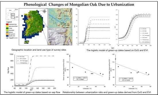
Figure 1.
A map showing the location of the study sites.

Figure 2.
A field of view from the digital camera at the Mt. Jeombong site. Regions of interest (ROIs) 1–3 are indicated in red.
Figure 2.
A field of view from the digital camera at the Mt. Jeombong site. Regions of interest (ROIs) 1–3 are indicated in red.

Figure 3.
(a,b) show the seasonal courses of ExG in the Mongolian oak stands of each site. (c) shows the logistic models of green-up based on ExG, and (d) shows the rate of change of curvature K in study sites. The time at which the rate of change in curvature exhibits local maxima indicates the green-up date.

Figure 4.
(a,b) show the seasonal courses of EVI in the Mongolian oak stands of each site. (c) shows the logistic models of green-up based on EVI, and (d) shows the rate of change of curvature K in study sites. The time at which the rate of change in curvature exhibits local maxima indicates the green-up date.

Figure 5.
Relationship between urbanization ratio and green-up dates derived from ExG (upper) and EVI (lower) (p < 0.05).
Figure 5.
Relationship between urbanization ratio and green-up dates derived from ExG (upper) and EVI (lower) (p < 0.05).

Figure 6.
Relationship between dates when AGDD reached 159 °C and urbanization ratio (p < 0.05).

Figure 7.
Changes in sap flow velocity during the study period in each site.

Figure 8.
SFM logistic models of green-up (a) and curvature K (b) in study.


Table 1.
Description of study sites. DoY: day of year.
| Site Name | Latitude (Decimal Degree) | Longitude (Decimal Degree) | Elevation (m) | Tower Type | Data Collection Period (DOY) | ||
|---|---|---|---|---|---|---|---|
| Digital Camera | MODIS | ||||||
| Urban center | Mt. Nam | 37.55 | 126.99 | 215 | Ecological tower | 56~240 | 2016/2/19 ~ 2016/7/18 |
| Mt. Mido | 37.49 | 127.00 | 40 | 56~240 | |||
| Mt. Umyeon | 37.47 | 127.00 | 185 | 76~240 | |||
| Suburb | Mt. Cheonggye | 37.44 | 127.05 | 276 | 72~240 | ||
| Mt. Buram | 37.63 | 127.09 | 115 | 63~240 | |||
| Rural area | Gwangneung (Mt. Sori) | 37.75 | 127.15 | 345 | Fire surveillance tower | 96~240 | |
| Natural area | Mt. Jeombong | 38.04 | 128.47 | 830 | Ecological tower | 91~240 | |
Table 2.
Urbanization rate in study sites.
| Site Name | Urbanized Area (km2) | Urbanization Rate (%) | |
|---|---|---|---|
| Urban center | Mt. Nam | 59.71 | 76.07 |
| Mt. Mido | 55.22 | 70.35 | |
| Mt. Umyeon | 41.16 | 52.44 | |
| Suburb | Mt. Cheonggye | 28.10 | 35.80 |
| Mt. Buram | 38.94 | 49.60 | |
| Rural area | Gwangneung (Mt. Sori) | 5.01 | 6.38 |
Table 3.
Descriptions of the intervalometers and cameras employed. FoV: field of view.
| Intervalometer | Daily Capture Times | 09:00, 12:30, 16:00 |
|---|---|---|
| Interval between Captures | 3 1/2 h | |
| Camera | Model | Acorn Ltl-6210M |
| Sensor | 5 megapixel color CMOS | |
| Pixel size | 2560 × 1920 | |
| Channels | RGB (red, green, blue) | |
| Lens | F = 3.1; FoV = 52; Auto IR-Cut | |
| Memory card | 32 GB SD | |
| File type | High-quality JPEG (2MP) | |
| Power | 12 × AA; Solar panel | |
| Flash | Disabled |
Table 4.
Green-up dates estimated by two different criteria, ExG and EVI, and the difference between observed and expected green-up dates from ExG and EVI. Obs: observed, Exp: expected, Diff: difference.
Table 4.
Green-up dates estimated by two different criteria, ExG and EVI, and the difference between observed and expected green-up dates from ExG and EVI. Obs: observed, Exp: expected, Diff: difference.
| Site | ExG | EVI | |||||
|---|---|---|---|---|---|---|---|
| Obs (DoY) | Exp (DoY) | Diff (Days) | Obs (DoY) | Exp (DoY) | Diff (Days) | ||
| Urban center | Mt. Nam | 94 | 110 | −16 | 94 | 110 | −16 |
| Mt. Mido | 95 | 113 | −18 | 96 | 114 | −18 | |
| Mt. Umyeon | 95 | 110 | −15 | 97 | 112 | −15 | |
| Suburb | Mt. Cheonggye | 97 | 111 | −14 | 96 | 110 | −14 |
| Mt. Buram | 95 | 110 | −15 | 96 | 111 | −15 | |
| Rural area | Gwangneung (Mt. Sori) | 103 | 114 | −11 | 104 | 115 | −11 |
| Natural area | Mt. Jeombong | 118 | 118 | 0 | 114 | 114 | 0 |
Table 5.
Green-up dates estimated by AGDD and AGDD values for green-up dates derived from ExG and EVI.
Table 5.
Green-up dates estimated by AGDD and AGDD values for green-up dates derived from ExG and EVI.
| Site Name | Green-Up Dates (DoY) | AGDD (°C) | ||
|---|---|---|---|---|
| ExG | EVI | |||
| Urban center | Mt. Nam | 94 | 160.3 | 160.3 |
| Mt. Mido | 95 | 158.2 | 166.9 | |
| Mt. Umyeon | 95 | 156.3 | 162.6 | |
| Suburb | Mt. Cheonggye | 97 | 162.2 | 153.2 |
| Mt. Buram | 96 | 162.3 | 168.3 | |
| Rural area | Gwangneung (Mt. Sori) | 103 | 156.6 | 163.3 |
| Natural area | Mt. Jeombong | 114 | 160.5 | 154.4 |
| Average | 159.5 | 161.3 | ||
Table 6.
Comparisons of green-up dates derived from vegetation phenology (ExG and EVI) and sap flow (SFM).
Table 6.
Comparisons of green-up dates derived from vegetation phenology (ExG and EVI) and sap flow (SFM).
| Site | ExG (DoY) | EVI (DoY) | SFM (DoY) | Difference (Days) | |
|---|---|---|---|---|---|
| ExG-SFM | EVI-SFM | ||||
| Mt. Nam | 94 | 94 | 94 | 0 | 0 |
| Mt. Mido | 95 | 96 | - | - | - |
| Mt. Umyeon | 95 | 97 | 96 | −1 | 1 |
| Mt. Cheonggye | 97 | 96 | 97 | 0 | 1 |
| Mt. Buram | 95 | 96 | - | - | - |
| Gwangneung (Mt. Sori) | 103 | 104 | 104 | 1 | 0 |
| Mt. Jeombong | 118 | 114 | - | - | - |
Publisher’s Note: MDPI stays neutral with regard to jurisdictional claims in published maps and institutional affiliations. |
© 2021 by the authors. Licensee MDPI, Basel, Switzerland. This article is an open access article distributed under the terms and conditions of the Creative Commons Attribution (CC BY) license (https://creativecommons.org/licenses/by/4.0/).
Share and Cite
MDPI and ACS Style
Kim, A.R.; Lim, C.H.; Lim, B.S.; Seol, J.; Lee, C.S. Phenological Changes of Mongolian Oak Depending on the Micro-Climate Changes Due to Urbanization. Remote Sens. 2021, 13, 1890. https://doi.org/10.3390/rs13101890
AMA Style
Kim AR, Lim CH, Lim BS, Seol J, Lee CS. Phenological Changes of Mongolian Oak Depending on the Micro-Climate Changes Due to Urbanization. Remote Sensing. 2021; 13(10):1890. https://doi.org/10.3390/rs13101890
Chicago/Turabian StyleKim, A Reum, Chi Hong Lim, Bong Soon Lim, Jaewon Seol, and Chang Seok Lee. 2021. "Phenological Changes of Mongolian Oak Depending on the Micro-Climate Changes Due to Urbanization" Remote Sensing 13, no. 10: 1890. https://doi.org/10.3390/rs13101890
Note that from the first issue of 2016, this journal uses article numbers instead of page numbers. See further details here.