Remote Sensing-Based Rainfall Variability for Warming and Cooling in Indo-Pacific Ocean with Intentional Statistical Simulations

Abstract

This study analyzed the sensitivity of rainfall patterns in South China and the Indochina Peninsula (ICP) using statistical simulations of observational data. Quantitative changes in rainfall patterns over the ICP were examined for both wet and dry seasons to identify hotspots sensitive to ocean warming in the Indo-Pacific sector. The rainfall variability was amplified by combined and/or independent effects of the El Niño–Southern Oscillation and the Indian Ocean Dipole (IOD). During the years of El Niño and a positive phase of the IOD, rainfall is less than usual in Thailand, Cambodia, southern Laos, and Vietnam. Conversely, during the years of La Niña and a negative phase of the IOD, rainfall throughout the ICP is above normal, except in parts of central Laos, northern Vietnam, and South China. This study also simulated the change of ICP rainfall in the wet and dry seasons with intentional IOD changes and verified IOD-sensitive hotspots through quantitative analysis. The results of this study provide a clear understanding both of the sensitivity of regional precipitation to the IOD and of the potential future impact of statistical changes regarding the IOD in terms of understanding regional impacts associated with precipitation in changing climates.

1. Introduction

Spatiotemporal variation in precipitation extremes can result from the amplification of changes in atmosphere–ocean interactions and the intensification of the hydrological cycle on both regional and global scales attributable to the effects of global climate change [1,2,3,4,5,6]. Changes in the magnitude and frequency of regional rainfall are closely related to the occurrence of floods and droughts. They have important implications not only in terms of their socioeconomic impact, but also in relation to the management of local and/or regional hydropower, irrigation, and environmental water resources [7,8,9]. The occurrence of extreme precipitation, which is highly likely to continue into the future, is increasingly regarded as an area of concern by the public because many countries have experienced such extreme events in recent years [7,10,11,12,13]. In particular, there has been rapid increase in both the amount of damage and the number of fatalities associated with the occurrence of extreme rainfall in developing countries because of their vulnerable infrastructure, high density of human activities, and poor land use practices and development ([14,15].

The El Niño–Southern Oscillation (ENSO) is known for its active and predictable short-term behavior within the global climate system [16], characterized by irregular but periodic changes in the behavior of winds and sea level temperatures over the tropical eastern Pacific Ocean. Since the 2000s, new forms of El Niño have appeared more frequently in the central Pacific [17,18]. However, little is yet known about the causes of these new types of El Niño, some of which have been reported to have a noticeable effect on the supply of warm seasonal freshwater and hydrological extremes in Pacific Rim countries [5,19,20,21,22]. Research over the past two decades has identified a distinct climate anomaly in the Indian Ocean, known as the Indian Ocean Dipole (IOD) [23,24,25,26]. The IOD is an atmosphere–ocean coupling mode characterized by the opposition of anomalies of sea surface temperature (SST) in the west and east of the tropical Indian Ocean [23,24,27]. A positive (negative) IOD pattern is characterized by water warmer (cooler) than normal in the western tropical Indian Ocean (10° S–10°N, 50°–70°E) and water cooler (warmer) than normal in the southeastern tropical Indian Ocean (10° S to the equator, 90°–110°E). These events usually begin around May or June and they terminate rapidly in early winter after reaching a peak between August and October [24]. Long-term climatic change has high correlation with large-scale atmospheric teleconnections and it has been reported to be predictable in relation to the behavior of nonlinear climate systems, particularly in terms of ocean-related climatic drivers such as ENSO and the IOD mode [23,24]. ENSO and IOD patterns are known as leading causes of large atmospheric change and they are related closely to seasonal variations in precipitation in the Indian Ocean region and around the world [18,28,29,30].

Recent studies have suggested that the observed slowdown in the rise of global mean surface atmospheric temperature is closely related to the considerable transport of heat from the Pacific Ocean into the Indian Ocean via the Indonesian Throughflow [31,32,33]. Investigation of Indo-Pacific thermocouples can help both to improve understanding of the regional-scale climatic variability that is globally relevant and to diagnose quantitatively such variability in a changing climate. However, there has been little previous quantitative research on rainfall variation across the Indochina Peninsula (ICP) in relation to IOD phenomena and ENSO evolution. Therefore, based on historical observations, this study undertook quantitative analysis of the changes in SST in the Indo-Pacific sector and the associated interseasonal variation of precipitation over the ICP. The study had three primary areas of interest: (1) the spatiotemporal changes in magnitude and frequency of precipitation during the dry and wet seasons, (2) the relationship between the changes in weather extremes and large-scale climatic patterns over the ICP, and (3) identification of IOD-sensitive hotspots using the intentionally biased bootstrapping (IBB) technique based on limited historical observations.

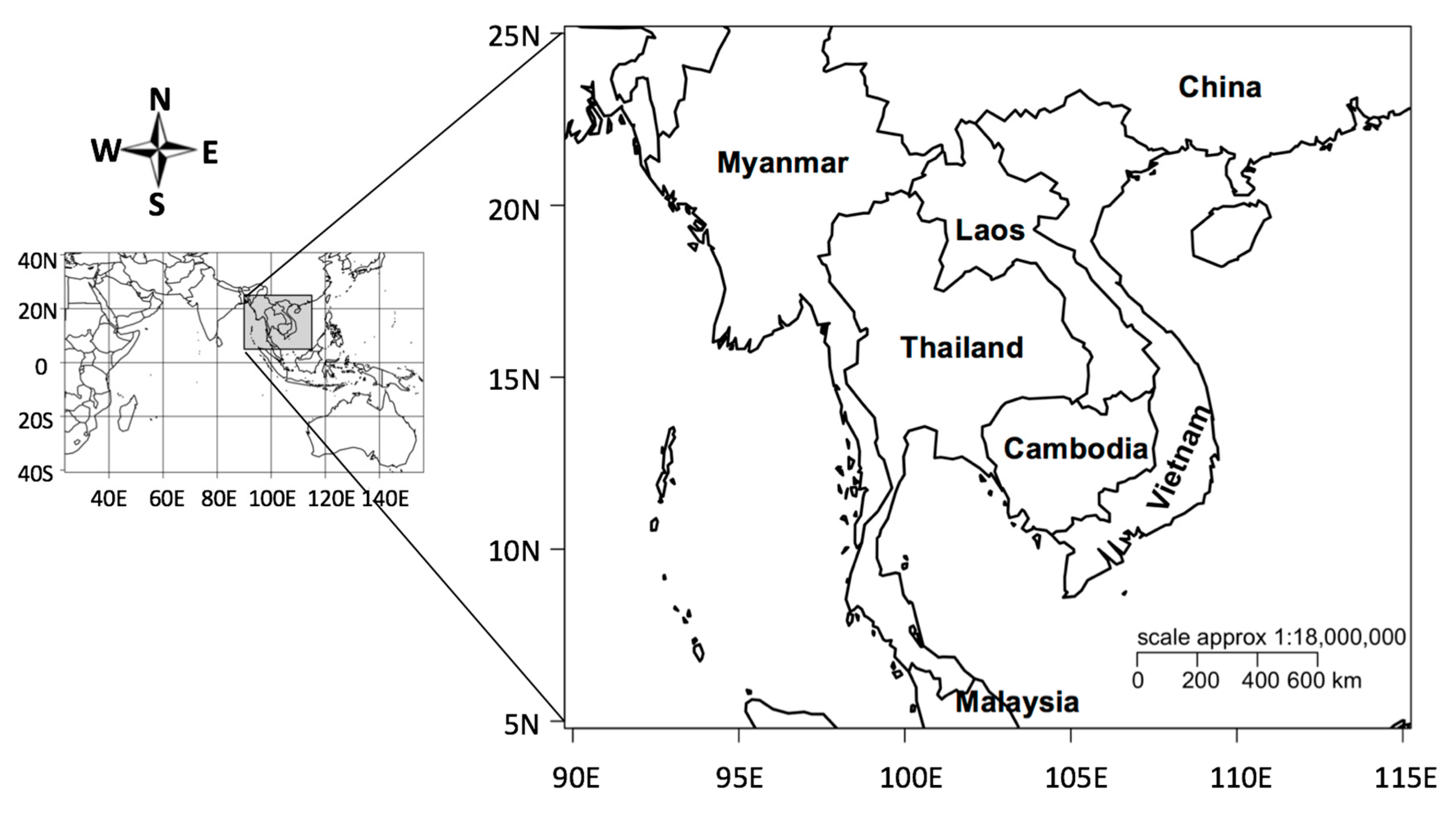
2. Materials and Methods

2.1. Precipitation Dataset and Climate Change Indices

This study used the high-resolution (0.5° × 0.5°) daily Climate Prediction Center Global Unified Precipitation dataset for 1979–2018, which was obtained from the website of NOAA’s Earth System Research Laboratory’s Physical Research Division (https://www.esrl.noaa.gov/psd/). The Global Precipitation Climatology Center monthly precipitation dataset with 1.0° × 1.0° spatial resolution for the period 1948–2018, which is based on quality-controlled data from 67,200 stations worldwide [34], was also used to identify seasonal precipitation variability over the ICP region (5°–25°N, 90°–115°E) (Figure 1). To identify changes in the frequency and intensity of rainfall, six major climate change indices [35], based on the daily Climate Prediction Center data from 1979–2018, were analyzed for both the wet season (May–October) and the dry season (November–April). These indices included the seasonal total precipitation (PRCPTOT) on wet days, seasonal total of the 95th percentile of precipitation (R95pTOT) on wet days (≥1.0 mm), seasonal maximum 1-day precipitation (RX1day), simple precipitation intensity index (SDII) with a daily precipitation amount on wet days of ≥1.0 mm, maximum number of consecutive dry days (CDD) with a daily precipitation amount of <1.0 mm, and maximum number of consecutive wet days (CWD) with a daily precipitation amount of ≥1.0 mm. Wet and dry days were calculated separately for both the wet season (May–October) and the dry season (November–April).

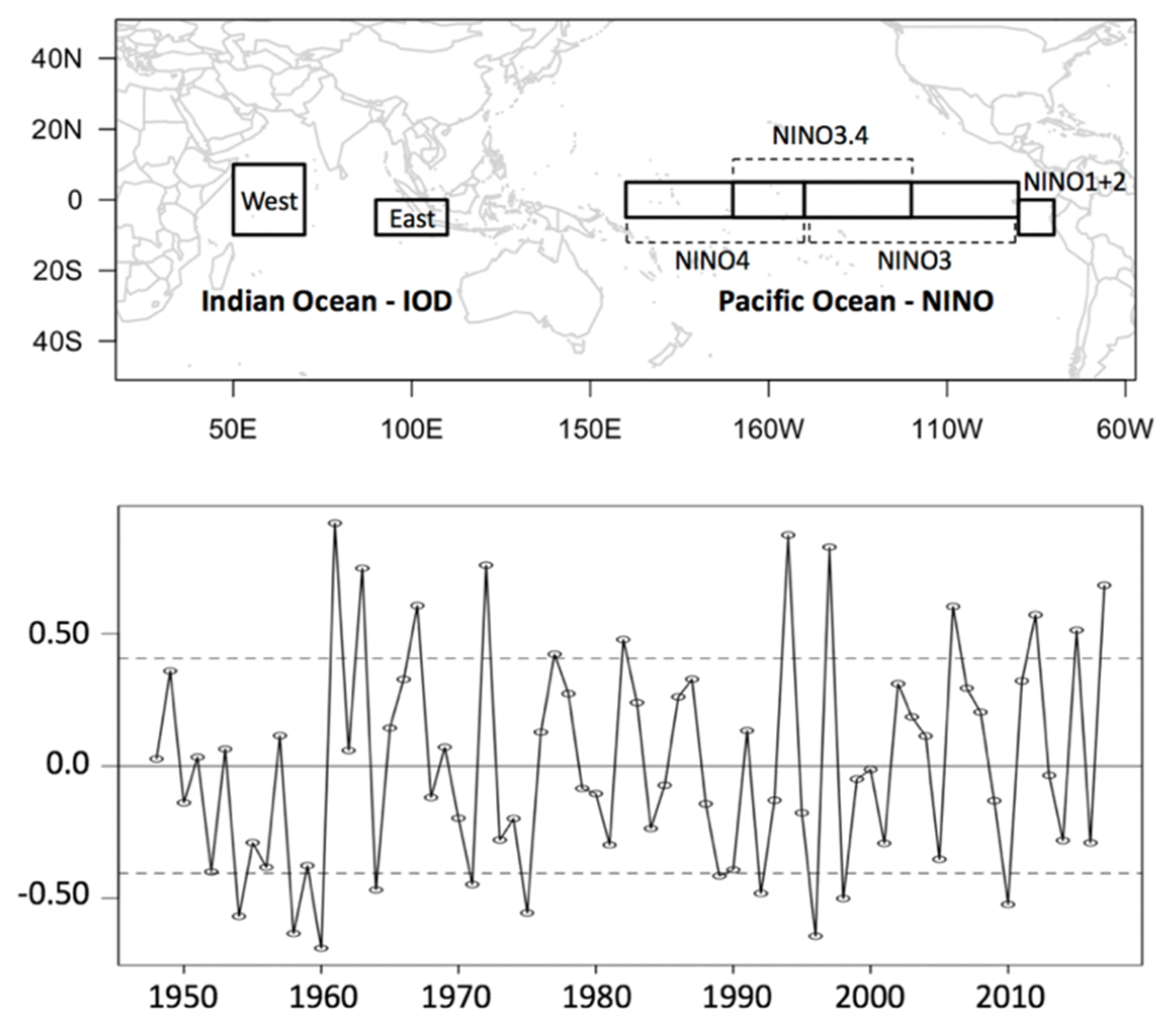
2.2. Indian Ocean Dipole (IOD) and El Niño–Southern Oscillation (ENSO)

The monthly SST anomaly (SSTA) from NOAA’s Extended Reconstructed Sea Surface Temperature (ERSST) dataset v5 in the Tropical Indian Ocean (TIO) was used to calculate the IOD mode index. This is defined as the SSTA difference between the western (10° S–10°N, 50°–70°E) and southeastern (10°S to the equator, 90°–110°E) regions of the TIO [24]. From 1948–2017, a 3-month running average was applied to the IOD mode index data (August–September–October), which is the peak phase period, with ±1 SD to determine the years with positive and negative modes of the IOD (Figure 2). To characterize different types of ENSO event, monthly Niño3 (5° S–5°N, 150°E–90°W) and Niño4 (5°S–5°N, 160°E–150°W) data for the period 1948–2018 were used for El Niño development phases (December–January–February).

In this study, the pattern of El Niño was divided into two groups depending on where the peak and persistent anomalies in SST occurred in the tropical Pacific: (1) Eastern Pacific (EP), El Niño occurring in the EP; and (2) Central Pacific (CP), El Niño emerging in the CP. This study employed two new indices (Equation (1)) to identify the two types of El Niño events through a simple transformation of the Niño3 and Niño4 indices, as proposed by Ren and Jin [36]:

$$\begin{array}{l}{N}_{CT}=N_3-\alpha N_4\\ N_{WP}=N_4-\alpha N_3,\end{array}\alpha =\{\begin{array}{c}0.4,N_3{N}_4>0\\ 0,otherwise.\end{array}$$

(1)

Here, N₃ and N₄ indicate the Niño3 and Niño4 indices, respectively.

Assessment of the relative impacts of the IOD and ENSO on rainfall across the ICP was based mainly on composite analyses. During the period 1979–2018, the effects of ENSO and the IOD were evaluated in terms of rainfall across the ICP during both the wet season (May–October) and the dry season (November–April).

2.3. Trend Detection

A nonparametric Mann–Kendall test is commonly used to detect a monotonic pattern in a time series of climate data based on the null hypothesis that the data are independent and sorted randomly [37,38]. The null hypothesis H₀ is random in the order of the sample data (X_i, i = 1, 2..., n) and it has no trend, whereas the alternative hypothesis H₁ represents the monotonous tendency of X. The S statistic for Kendall’s tau is calculated as follows:

$$\mathrm{S}=\underset{\mathrm{i}=1}{\overset{\mathrm{n}-1}{\_}}\underset{\mathrm{j}=\mathrm{i}+1}{\overset{\mathrm{n}}{\_}}\mathrm{sgn}\left({\mathrm{X}}_{\mathrm{j}}-{\mathrm{X}}_{\mathrm{i}}\right)$$

(2)

and

$$\mathrm{sgn}(\_)=\{\begin{array}{lll}1& & \mathrm{if}\_>0\\ 0& & \mathrm{if}\_=0\\ -1& & \mathrm{if}\_<0\end{array}.$$

(3)

The S statistic is calculated using the following mean and variance:

$$\mathrm{E}\left(\mathrm{S}\right)=0,$$

(4)

$$\mathrm{V}\left(\mathrm{S}\right)=\frac{\mathrm{n}\left(\mathrm{n}-1\right)\left(2\mathrm{n}+5\right)-{–}_{\mathrm{m}=1}^{\mathrm{n}}{\mathrm{t}}_{\mathrm{m}}\mathrm{m}\left(\mathrm{m}-1\right)\left(2\mathrm{m}+5\right)}{18}$$

(5)

where t_m measures the ties of extent m. The standardized test statistic Z is estimated as follows:

$$\mathrm{Z}=\{\begin{array}{ccc}\frac{\mathrm{S}-1}{\sqrt{\mathrm{V}\left(\mathrm{S}\right)}}& & \mathrm{S}>0\\ 0& & \mathrm{S}=0\\ \frac{\mathrm{S}+1}{\sqrt{\mathrm{V}\left(\mathrm{S}\right)}}& & \mathrm{S}<0\end{array}.$$

(6)

The existence of autocorrelation in a dataset affects the probability of detecting a trend when it does not exist and vice versa, but this is often ignored. Thus, the modified nonparametric trend test developed by Hamed and Rao [39] was applied in this study. The corrected Z value is derived as follows:

$$\mathrm{Z}=\{\begin{array}{ccc}\frac{\mathrm{S}-1}{\sqrt{{\mathrm{V}}^{*}\left(\mathrm{S}\right)}}& & \mathrm{S}>0\\ 0& & \mathrm{S}=0\\ \frac{\mathrm{S}+1}{\sqrt{{\mathrm{V}}^{*}\left(\mathrm{S}\right)}}& & \mathrm{S}<0\end{array}$$

(7)

where

$$V^{*}\left(S\right)=V\left(S\right)\ast \frac{n}{n_S^{*}}$$

(8)

$$\frac{n}{n_S^{*}}=1+\frac{2}{n\left(n-1\right)\left(n-2\right)}\ast \underset{i=1}{\overset{n-1}{\_}}\left(n-i\right)\left(n-i-1\right)\left(n-i-2\right){\_}_S\left(i\right)$$

(9)

and where ${\_}_S\left(i\right)$ is an autocorrelation function of the rank with respect to the observations. The sign of Z represents the trend direction, and the magnitude of Z is associated with the significance level, where |Z| > 1.64 for the 10% significance level and |Z| > 1.96 for the 5% significance level.

2.4. Intentionally Biased Bootstrapping Method

Bootstrapping analysis is a statistical method that can generate replicated datasets from source data, and it can evaluate the variability of their quantiles without performing separate analytical calculations [40]. However, the intentionally biased bootstrapping (IBB) technique applied in this study is a method that allows assessment of the relative effects of a response variable by deliberately increasing or decreasing the mean of the explanatory variable to a certain level while resampling it with the response variable [41].

Figure 3 shows the IBB resampling process applied in this study, and a brief description of the IBB analysis process is given below.

Among n observations $x_i$ ($i=1,2,3,\dots ,n$), suppose that the mean of the generated data is deliberately increased or decreased by $\Delta \mu$ for resampling of the observations with bootstrapping. As a result, high (low) values are likely to be resampled and low (high) values could be less likely to be selected. Thus, IBB can be obtained by allocating different weights $S_{i,n}$ depending on the following observation values (Equation (10)):

$$S_{i,n}=i/n.$$

(10)

The weight $S_{i,n}$ assigned after scaling and adjustment contributes to the probability of selection for the data observed in the IBB procedure. The average of the resampled data can be expressed as in Equation (11):

$$\tilde{\mu }=\frac{1}{\psi }{\sum }_{i=1}^n{S}_{i,n}{x}_i$$

(11)

where $x_i$ represents the $i$-th incremental value and $\psi ={\sum }_{i=1}^n{S}_{i,n}$. The average amount of increase or decrease $\Delta \mu$ is shown in Equation (12):

$$\Delta \mu =\frac{1}{\psi }{\sum }_{i=1}^n{S}_{i,n}{x}_i-\frac{1}{n}{\sum }_{i=1}^n{x}_i.$$

(12)

To obtain another value of $\Delta \mu$, the weights can be regeneralized in the order of the weight sequence ($r$); thus, $\Delta \tilde{\mu }\left(r\right)$ is derived as follows:

$$\Delta \tilde{\mu }\left(r\right)=\tilde{\mu }\left(r\right)-\widehat{\mu }=\frac{1}{{\psi }_r}{\sum }_{i=1}^n{s}_{i,n}^r{x}_i-\frac{1}{n}{\sum }_{i=1}^n{x}_i.$$

(13)

If the average value of increase or decrease is given as $\Delta \mu$, then the weight “$r$” can be calculated accordingly. In this study, the selection of the weight sequence was performed using a Self-Organizing Migrating Algorithm with the objective function to minimize ${\left[\Delta \mu -\Delta \tilde{\mu }\left(r\right)\right]}^2$. This approach follows a past study of extreme droughts during spring (March–May) in the Indochina peninsula [42]; however, no climate change indices for both the wet season (May–October) and the dry season (November–April) were integrated in that study, taking into account both the dipole mode in the tropical Indian Ocean and SST warming in the Pacific Ocean. In addition, the IBB technique was employed to generate resampled datasets for the IOD and the response to the intensity and frequency of rainfall in order to identify IOD-sensitive hotspots over the ICP. The statistical significance of the analysis results was assessed using the significance level of the 95th percentile.

3. Results

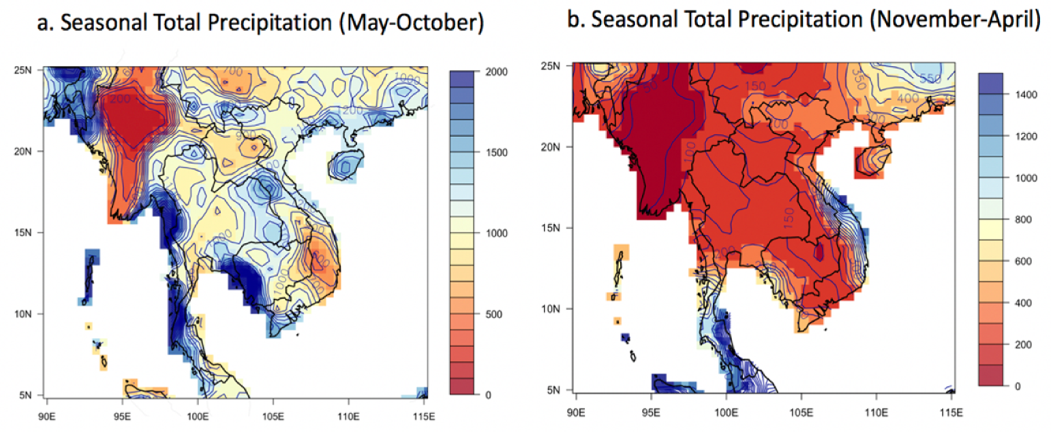
3.1. Seasonal Precipitation Patterns across the ICP

The ICP is a region in which monsoon rains occur in different seasons in association with seasonal winds and mountain areas. Geographically, the ICP has the Arakan Mountains in the west, the Bilauktung Mountains and the Dawna Mountains in the center, and the Annamese Mountains in the east. Meteorologically, the ICP is divided into three monsoon periods: the southwest monsoon during June–November, southeast monsoon during September–November, and northeast monsoon during November–February. This study considered the wet season (May–October) and the dry season (November–April) to identify the potential impact on regional rainfall associated with atmosphere–ocean feedback in the Indian and Pacific oceans.

Figure 4 shows the seasonal average precipitation during the wet and dry seasons across the ICP region during 1979–2018. The total precipitation during the wet season across the ICP is about 1000–1500 mm. In addition, it has been confirmed that precipitation variability is dependent on specific regions (Figure 4a). The precipitation variability was found to differ significantly between inland (<1000 mm) and coastal areas (>2000 mm). Precipitation on the western coast of Cambodia, the coast of western Thailand, and Myanmar during June–November is attributable to the influence of the southwest and southeast monsoons. Moreover, a clear difference in precipitation is evident between eastern and western parts of the Arakan Mountains in Myanmar. As water vapor from Bangorman decreases over the mountains, the Arakan Mountains show an arid climate to the east and a pattern of strong precipitation to the west.

During the dry season, total precipitation across the ICP is about 150–200 mm, indicating that rainfall variability is not significantly dependent on specific regions (Figure 4b). In particular, in the dry season, because of the influence of the northeast monsoon during November–February, high rainfall is received in central coastal areas of Vietnam, e.g., near the city of Danang. Similarly, in the case of Myanmar, eastern parts are dry because of the influence of the Arakan Mountains. The climatic characteristics of the ICP are distinctive not only because of the effects of monsoons and mountain areas, but also because of the characteristics of local areas and because of specific temporal effects. The precipitation patterns of the ICP are likely to change according to the characteristics of the wet and dry seasons, as well as because of the influence of ocean-related climate factors (e.g., the IOD and ENSO).

3.2. Spatiotemporal Variation in Precipitation over the ICP

Figure 5 and Figure 6 illustrate the long-term trend of precipitation over the ICP during the period 1979–2018 for the wet and dry seasons, respectively. They show the results of the six major climate change indices that represent the magnitude and frequency of precipitation. For each figure, the direction of the trend is displayed in blue (increase) and red (decrease). Figure 5a,b and Figure 6a,b show the long-term trends of PRCPTOT and R95pTOT. These seasonal indices can be used to assess total precipitation. It can be seen that the characteristics of their spatial distribution are similar. During the wet season, there is a noticeable decrease in precipitation at the 5–10% significance level in northern Cambodia, some parts of Laos, and southern Thailand. In addition, it can be seen that there is a marked trend of increase at the 5–10% significance level in northwestern Myanmar, parts of western Thailand, central Vietnam, and southern parts of China (Figure 5a,b).

During the dry season, there is a noticeable increase in precipitation at the 5–10% significance level along eastern and southern coastal areas of the ICP (i.e., Vietnam and Cambodia) and some southern coastal regions of Thailand (Figure 6a,b). The R95pTOT climate index also shows a trend of increase in precipitation to the west of the Arakan Mountains in Myanmar (Figure 6b). Therefore, long-term changes in the pattern of precipitation across the ICP during the wet season show a trend of decrease (increase) in central inland areas (some coastal areas). During the dry season, there is a general trend of increase in precipitation across the ICP. Notably, the trend of increase in precipitation in southeastern coastal areas appears significant.

Figure 5c,d and Figure 6c,d illustrate the long-term trends in RX1day and SDII. The RX1day and SDII climate indices can be used to assess rainfall intensity. It can be seen that the characteristics of the spatial distribution of the two indices are similar. Moreover, the characteristics of their spatial distribution are also similar to PRCPTOT and R95pTOT. It can be seen that during the rainy season the intensity of rainfall in central and northern Myanmar, central and southern Vietnam, and southern China increases, whereas the rainfall intensity decreases in Laos, Cambodia, northeastern Myanmar, and South Vietnam. During the dry season, rainfall intensity generally increases across the ICP, although it shows a clear pattern of decrease in Laos, as in the wet season.

Figure 5e,f, and Figure 6e,f show the long-term trends in CDD and CWD. The CDD and CWD indices can be used in assessment of droughts and floods, respectively. Therefore, it is unsurprising that the CDD and CWD indices exhibit opposite spatial distribution characteristics. During the rainy season, the CDD value across the ICP largely tends to increase, although it decreases in some coastal areas, e.g., Vietnam. The CWD index shows the reverse tendency.

During the dry season, an increase (decrease) of the CDD (CWD) index can be clearly observed at the 5–10% significance level (Figure 6e,f). The CDD index increases along the southeast coast of the ICP, e.g., in areas of Vietnam, Cambodia, and southern Thailand, whereas the CWD index exhibits the opposite trend. An increase (decrease) in the CDD index suggests that drought is more (less) likely to occur, while a decrease (increase) in the CWD index means that the occurrence of drought is less (more) likely. Therefore, during the rainy season, floods are expected to increase along the southeastern coast of the ICP (e.g., in Vietnam, Cambodia, and Thailand), while drought is more likely to occur during the dry season.

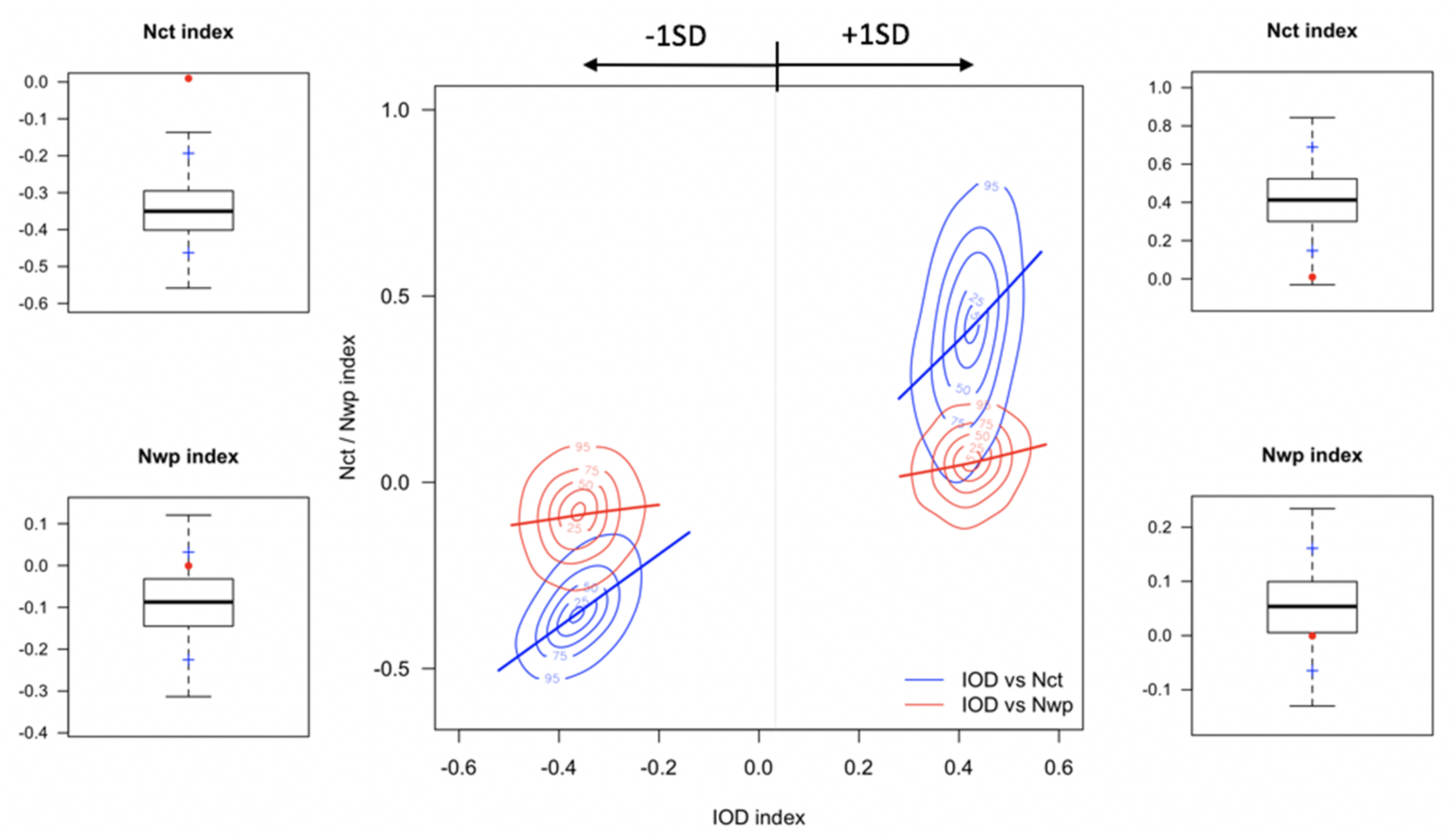
3.3. Precipitation Variability Associated With the IOD and ENSO

The IOD, Asian monsoon, and other regional climatological patterns can lead to local or global climate change, particularly in Indian Ocean Rim countries, which can cause severe flooding or droughts depending on IOD variability [26]. Composite analysis can clarify the role of the Southeast Asian Summer Monsoon in precipitation variability across the ICP region associated with years of strong IOD and ENSO after identifying that tropical climate phenomena are the main factors that influence precipitation variability over the ICP during the wet and dry seasons. However, this role differs depending on the combination of the two climate phenomena and on the season.

Figure 7 shows the results of composite rainfall anomalies (shown as a percentage relative to normal) over the ICP during the wet and dry seasons in relation to the IOD and ENSO. The patterns of rainfall anomalies indicate significant difference between positive and negative IOD years. For positive IOD years, the wet season rainfall (Figure 7a) shows a decrease of <20% in southern parts of the ICP, whereas there is a marked increase in rainfall centered over the Arakan Mountains in western Myanmar. It can be seen that the amount of rainfall received during the dry season (Figure 7c) is similar to that in the wet season, but there is 40–50% less rainfall than usual in certain mainland regions of Southeast Asia, especially Yangon and Mawlamyine in Myanmar and in eastern Cambodia.

In negative IOD years, intense positive anomalies of rainfall can be seen in central Cambodia and southern parts of Vietnam. A slight strong-pitched anomaly pattern is evident during the wet season (Figure 7b) around the coastline of both Bangladesh and Myanmar, whereas weak-pitched positive anomalies (about 10–15% relative to the long-term average) are found throughout the ICP. However, changes in rainfall pattern are not evident during the dry season (Figure 7d), and although the amount varies depending on region, rainfall is generally >30–50% above the long-term average. As in the wet season, the dry season also shows relatively strong positive rainfall patterns with positive anomalies of >80–100% in Cambodia and both central and southern Vietnam.

Sometimes droughts and flooding are likely to converge because of remote connections during IOD–ENSO periods, and they can have a significant impact on the modulation of the large-scale oceanic and atmospheric environment, especially in the Indian Ocean and in Pacific Rim countries [25,26,43]. Thus, consideration of both combined and independent effects of ENSO and the IOD on seasonal precipitation variability can provide improved predictive expertise, and reveal new insight into tropical climate change and global warming impacts [28].

Figure 8 shows composite rainfall anomalies (November–April) during positive and negative IOD years that coincided with ENSO. During positive IOD and El Niño years (Figure 8a), there is less rainfall than usual across Thailand, Cambodia, southern Laos, and Vietnam. In particular, southern regions of Myanmar (from Yangon to Mawlamyine) that border the Andaman Sea show a distinct decrease in rainfall by more than 50% in comparison with the long-term mean (1981–2010). However, in contrast, there is 20–40% more rainfall than usual in northern parts of the ICP, e.g., northern Myanmar (around 97E, 22N), northeastern parts of Laos (around 102E, 21N), and Vietnam. Furthermore, in Guangzhou in China, rainfall is up to 60% higher in comparison with average years. These rainfall signals are stronger in WP El Niño years than in CT El Niño years (figures not shown). During negative IOD and La Niña years (Figure 8b), rainfall above the long-term average is observed throughout the ICP, except for parts of central Laos (around 105E, 17N) and northern Vietnam (around 107E, 21N). The pattern of increased rainfall appears strongly throughout Myanmar and regions around Ho Chi Minh City in Vietnam. However, in the region adjacent to India and Bangladesh, as well as the Shenzhen area of China, strong negative anomalies are evident.

3.4. Identification of IOD-Sensitive Hotspots through IBB Simulations

Section 3.3 discussed the significant impact on rainfall anomalies in the ICP that are attributable to the combined or independent effects of ENSO and the IOD. In particular, both positive IOD events with El Niño and negative IOD events with La Niña interact in modulating rainfall anomalies over the ICP. The IOD and ENSO are strongly correlated, and their variations are mutually forced or triggered [43,44]. For the period of 1979–2018, the correlation between the peak phase of the IOD and the two types of El Niño index proposed by Ren and Jin [36] was analyzed. The results showed that the IOD has a strong positive correlation with the CT El Niño (N_CT) (ρ = 0.4850, p-value = 0.0018). However, the IOD also has positive correlation with the WP El Niño (N_WP), but not at a statistically significant level (ρ = 0.110, p-value = 0.5013). These results are also reflected in the results of the IBB simulation (Figure 9). Figure 9 shows the results of 1000 simulations for the N_CT and N_WP indices performed by applying the IBB technique to the IOD index based on historical observations for the period of 1979–2017. By applying a +1 SD increase of the IOD, the mean difference between the observation of N_CT and simulated N_CT shows a statistically significant increase at the 95% significance level (diff. = 0.392, Interquartile range (IQR) = 0.228). However, the difference in the mean value of the N_WP index, although increased slightly, is not statistically significant (diff. = 0.097, IQR = 0.094). By applying a −1 SD decrease of the IOD, the simulation results show changes similar to the case with a +1 SD increase of the IOD (N_CT: diff. = 0.360, IQR = 0.108, N_WP: diff. = 0.088, IQR = 0.098). Therefore, for changes in the IOD, the linear increase (or decrease) in the N_CT index is more pronounced than the change in the N_WP index.

The spatiotemporal connection between SST and winds shows strong coupling through precipitation and ocean dynamics [24]. This dipole mode accounts for about 12% of SST variability in the Indian Ocean, and its duration of activity can greatly affect both the intensity and the frequency of rainfall in the Indian Ocean Rim countries, including the ICP. Based on statistical simulations of historical observations (1979–2018), Figure 10 and Figure 11 show rainfall variation and the most sensitive hotspot areas in the wet and dry seasons of the ICP attributable to IOD changes.

The spatial distribution of differences in PRCPTOT is shown in Figure 10, given the condition of increases or decreases by 0.25 SD of the IOD index in the wet season. For a +1 SD increase of the IOD, PRCPTOT is >90% higher than usual throughout Myanmar, and weak positive anomaly patterns are evident in southwestern China. In contrast, a pattern of decrease of PRCPTOT of 15–20% less than the long-term average is evident in Cambodia and southern Vietnam, i.e., in areas of the downstream reaches of the Mekong River. However, no statistically significant changes occur in the central ICP region, except in some parts of central Laos and Thailand. This spatial distribution of rainfall anomaly is also found for the RX1day index, although occasional patterns of increase or decrease are evident and the spatial extent is reduced. In addition, throughout Myanmar, the CDD index is decreased by >25% in comparison with the long-term average year, while the CWD index is increased by 35–50%. For the CDD index, a statistically significant pattern of decrease is found across Vietnam, Cambodia, and Laos. The most significant changes in the CWD index are across Myanmar (increase of 35–50%), southern Cambodia, and the southeast coast of Vietnam (decrease of 15–20%). The other ICP regions generally show a pattern of weak increase in terms of CWD. For a −1 SD decrease of the IOD, PRCPTOT, RX1day, and CWD all show distinct patterns of increase in the Laos and Vietnam basins, while the CDD index shows a predominant pattern of decrease, except in certain areas. Analysis indicates that other regions have a reverse pattern compared with the case of the +1 SD increase of the IOD. Consequently, it is determined that changes in rainfall during the wet season in the ICP region are sensitive to changes in the IOD.

Given the condition of increases or decreases by 0.25 SD of the IOD index for the dry season, the spatial distribution of the rainfall indices is shown in Figure 11. For a decrease of −1 SD of the IOD, there is more rainfall (PRCPTOT and RX1day) than usual throughout the ICP, especially in Laos and Vietnam. For a +1 SD increase of the IOD, negative anomaly patterns of PRCPTOT are dominant in southern Vietnam, eastern Cambodia, and northeastern Thailand, while weak patterns of positive anomaly are evident in areas of Myanmar and South China. Compared with the changes in the rainfall indices during the wet season, changes in the rainfall indices are intensified and the spatial influence is more extensive. However, for the CDD and CWD indices, either the positive anomaly patterns are weakened or the negative anomaly patterns appear for a +1 SD increase of the IOD. Especially for the CWD index, a pattern of decrease by more than 10–20% compared with the long-term average is found in Thailand, whereas the Myanmar region shows a pattern of increase of 15–25%. In this study, we simulated the changes in both wet and dry season rainfall across the ICP according to intentional IOD changes, and IOD-sensitive hotspots were verified through quantitative analysis. The findings of this study could help elucidate the long-term changes in rainfall expected in the ICP region in a changing climate.

4. Summary and Conclusions

This study analyzed changes in the magnitude and frequency of precipitation during the dry and wet seasons over the ICP, taking into account both the dipole mode in the tropical Indian Ocean and SST warming in the Pacific Ocean. The main results are summarized as follows.

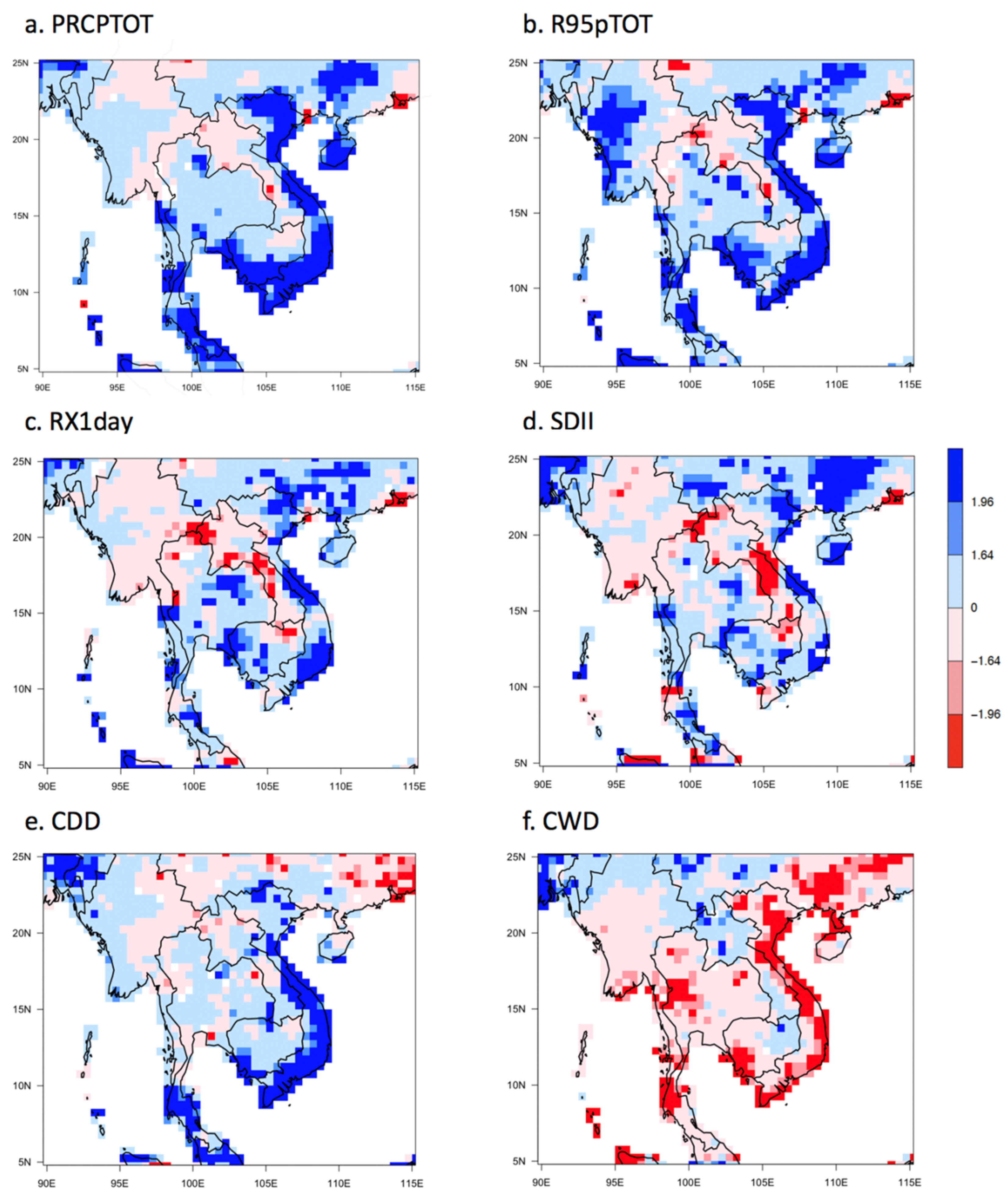
• According to analyses of the long-term trend in seasonal rainfall across the ICP during 1979–2018, rainfall showed significant decreases in northern Cambodia, parts of Laos, and southern Thailand during the wet season (May–October). Moreover, significant increases were evident in northwestern Myanmar, some parts of western Thailand, central Vietnam, and southern China. During the dry season (November–April), PRCPTOT rose noticeably in eastern and southern coastal areas of the ICP (i.e., Vietnam and Cambodia) and some southern coastal regions of Thailand.
• During the wet season, the CDD index increased or decreased in some coastal areas such as Vietnam. However, during the dry season, increases in CDD and decreases in CWD were evident in the ICP. In particular, a pattern of decline in CWD dominated southeastern coastal areas of the ICP, including Vietnam, Cambodia, and southern Thailand.
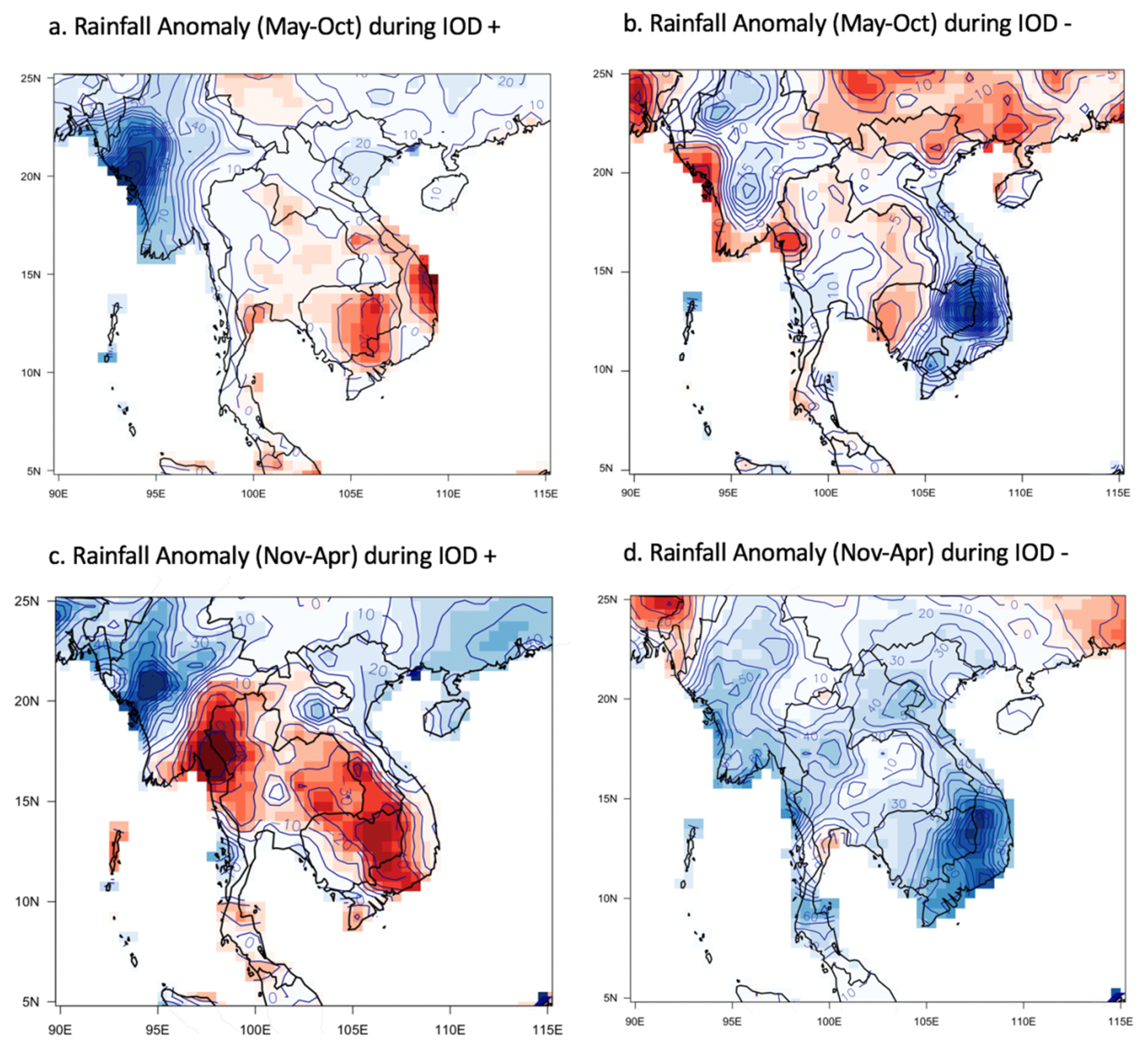
• The IOD showed strong positive correlation with the CT El Niño. However, although the IOD exhibited positive correlation with the WP El Niño, the relationship was not statistically significant. The variability of rainfall pattern and amount across the ICP was confirmed to be amplified by combined and independent effects of ENSO and the IOD. During years of positive IOD and El Niño, there was less rainfall than usual throughout Thailand and Cambodia, southern Laos, and Vietnam. In particular, the southern part of Myanmar, which borders the Andaman Sea, showed a decrease in regional rainfall of >50% in comparison with the long-term average. In contrast, northern parts of India and China, including Myanmar, northeastern Laos, and Vietnam, received 20–40% more rainfall than usual. Years with a negative IOD mode and La Niña showed rainfall above the long-term average across the ICP, except for certain parts, e.g., Central Laos and northern Vietnam.
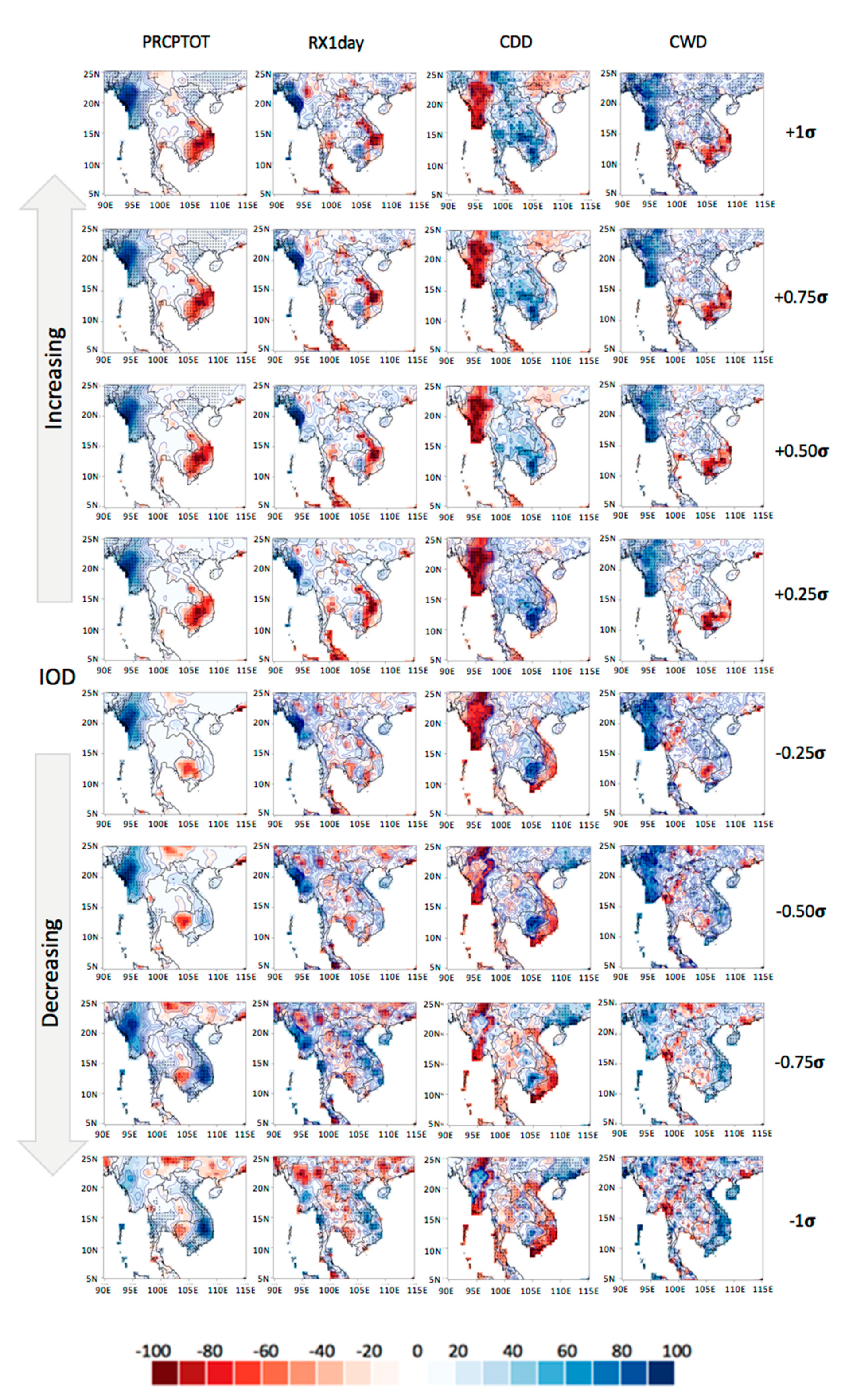
• Through application of the IBB technique, this study simulated the change of rainfall pattern and amount across the ICP for the wet and dry seasons according to intentional IOD changes, and IOD-sensitive hotspots were verified through quantitative analysis. For the wet season, a +1 SD increase of the IOD resulted in >90% more PRCPTOT than usual across Myanmar in the northwestern ICP. Conversely, in Cambodia and southern Vietnam, rainfall patterns were 15–20% less than the long-term average in the region of the lower Mekong River. In addition, the CDD index decreased throughout Myanmar by >25% compared with the long-term average. The most significant change in the CWD index was in Myanmar, i.e., a 35–50% increase. However, a pattern of decrease appeared across the southeastern coast of the ICP in southern Cambodia and Vietnam. For a +1 SD increase of the IOD in the dry season, negative anomaly patterns of PRCPTOT were found to be dominant in South Vietnam, eastern Cambodia, and northeastern Thailand, and more rainfall than usual occurred throughout the ICP, especially in Laos and Vietnam, when considering a −1 SD decrease of the IOD.

Although the results of this study are based on limited observations, they provide a clear perspective on the sensitivity of local precipitation to atmosphere–ocean interactions, and they reveal the potential future impact of statistical changes to the IOD, improving our understanding of the associated regional impact on precipitation under the effects of climate change.

References

1. Allan, R.P.; Soden, B.J. Atmospheric warming and the amplification of precipitation extremes. Science 2008, 321, 1481–1484. [Google Scholar] [CrossRef] [PubMed] [Green Version]
2. Kim, J.S.; Jain, S. Precipitation trends over the Korean peninsula: Typhoon-induced changes and a typology for characterizing climate-related risk. Environ. Res. Lett. 2011, 6, 034033. [Google Scholar] [CrossRef]
3. Ge, F.; Zhi, X.; Babar, Z.A.; Tang, W.; Chen, P. Interannual variability of summer monsoon precipitation over the Indochina Peninsula in association with ENSO. Theor. Appl. Climatol. 2017, 128, 523–531. [Google Scholar] [CrossRef]
4. Kang, H.Y.; Kim, J.S.; Kim, S.Y.; Moon, Y.I. Changes in High-and Low-Flow Regimes: A Diagnostic Analysis of Tropical Cyclones in the Western North Pacific. Water Resour. Manag. 2017, 31, 3939–3951. [Google Scholar] [CrossRef]
5. Kim, J.S.; Son, C.Y.; Moon, Y.I.; Lee, J.H. Seasonal rainfall variability in Korea within the context of different evolution patterns of the central Pacific El Niño. J. Water Clim. Chang. 2017, 8, 412–422. [Google Scholar] [CrossRef]
6. Gao, Q.; Kim, J.S.; Chen, J.; Chen, H.; Lee, J.H. Atmospheric Teleconnection-Based Extreme Drought Prediction in the Core Drought Region in China. Water 2019, 11, 232. [Google Scholar] [CrossRef]
7. Chi, X.; Yin, Z.; Wang, X.; Sun, Y. Spatiotemporal variations of precipitation extremes of China during the past 50 years (1960–2009). Theor. Appl. Climatol. 2016, 124, 555–564. [Google Scholar] [CrossRef]
8. Gu, X.; Zhang, Q.; Singh, V.P.; Shi, P. Changes in magnitude and frequency of heavy precipitation across China and its potential links to summer temperature. J. Hydrol. 2017, 547, 718–731. [Google Scholar] [CrossRef] [Green Version]
9. Choi, J.H.; Yoon, T.H.; Kim, J.S.; Moon, Y.I. Dam rehabilitation assessment using the Delphi-AHP method for adapting to climate change. J. Water Resour. Plan. Manag. 2018, 144, 06017007. [Google Scholar] [CrossRef]
10. Croitoru, A.E.; Chiotoroiu, B.C.; Todorova, V.I.; Torică, V. Changes in precipitation extremes on the Black Sea Western Coast. Glob. Planet. Chang. 2013, 102, 10–19. [Google Scholar] [CrossRef]
11. IPCC: Climate change 2013: The Physical Science Basis. Contribution of Working Group I to the Fifth Assessment Report of the Intergovernmental Panel on Climate Change; Cambridge University Press: Cambridge, UK, 2013. [Google Scholar]
12. Hirsch, R.M.; Archfield, S.A. Flood trends: Not higher but more often. Nat. Clim. Chang. 2015, 5, 198. [Google Scholar] [CrossRef]
13. Donat, M.G.; Lowry, A.L.; Alexander, L.V.; O’Gorman, P.A.; Maher, N. More extreme precipitation in the world’s dry and wet regions. Nat. Clim. Chang. 2016, 6, 508–514. [Google Scholar] [CrossRef]
14. Mirza, M.M.Q. Climate change and extreme weather events: Can developing countries adapt? Clim. Policy 2003, 3, 233–248. [Google Scholar] [CrossRef]
15. Yin, J.; Yin, Z.E.; Zhong, H.D.; Xu, S.Y.; Hu, X.M.; Wang, J.; Wu, J.P. Monitoring urban expansion and land use/land cover changes of Shanghai metropolitan area during the transitional economy (1979–2009) in China. Environ. Monit. Assess. 2011, 177, 609–621. [Google Scholar] [CrossRef] [PubMed]
16. Chen, D.; Cane, M.A. El Niño prediction and predictability. J. Comput. Phys. 2008, 227, 3625–3640. [Google Scholar] [CrossRef]
17. Ashok, K.; Yamagata, T. The El Niño with a difference. Nature 2009, 461, 481–484. [Google Scholar] [CrossRef]
18. Pradhan, P.K.; Preethi, B.; Ashok, K.; Krishna, R.; Sahai, A.K. Modoki, Indian Ocean Dipole, and western North Pacific typhoons: Possible implications for extreme events. J. Geophys. Res. 2011, 116, D18108. [Google Scholar] [CrossRef]
19. Kim, J.S.; Zhou, W.; Wang, X.; Jain, S. El Nino Modoki and the summer precipitation variability over South Korea: A diagnostic study. J. Meteorol. Soc. Jpn. 2012, 90, 673–684. [Google Scholar] [CrossRef] [Green Version]
20. Yoon, S.K.; Kim, J.S.; Lee, J.H.; Moon, Y.I. Hydrometeorological variability in the Korean Han River Basin and its sub-watersheds during different El Niño phases. Stoch. Environ. Res. Risk Assess. 2013, 27, 1465–1477. [Google Scholar] [CrossRef]
21. Son, C.Y.; Kim, J.S.; Moon, Y.I.; Lee, J.H. Characteristics of tropical cyclone-induced precipitation over the Korean River basins according to three evolution patterns of the Central-Pacific El Niño. Stoch. Environ. Res. Risk Assess. 2014, 28, 1147–1156. [Google Scholar] [CrossRef]
22. Wang, X.; Zhou, W.; Li, C.Y.; Wang, D.X. Comparison of the impact of two types of El Niño on tropical cyclone genesis over the South China Sea. Int. J. Climatol. 2014, 34, 2651–2660. [Google Scholar] [CrossRef]
23. Piechota, T.C.; Chiew, F.H.S.; Dracup, J.A.; McMachon, T.A. Seasonal streamflow forecasting in eastern Australia and the El Niño-Southern Oscillation. Water Res. Res. 1998, 34, 3035–3044. [Google Scholar] [CrossRef]
24. Saji, N.H.; Goswami, B.N.; Vinayachandran, P.N.; Yamagata, T. A Dipole Mode in the tropical Indian Ocean. Nature 1999, 401, 360363. [Google Scholar] [CrossRef] [PubMed]
25. Mahala, B.K.; Nayak, B.K.; Mohanty, P.K. Impacts of ENSO and IOD on tropical cyclone activity in the Bay of Bengal. Nat. Hazards 2015, 75, 1105–1125. [Google Scholar] [CrossRef]
26. Iqbal, A.; Hassan, S.A. ENSO and IOD analysis on the occurrence of floods in Pakistan. Nat. Hazards 2018, 91, 879–890. [Google Scholar] [CrossRef]
27. Webster, P.J.; Moore, A.M.; Loschnigg, J.P.; Leben, R.R. Coupled ocean–atmosphere dynamics in the Indian Ocean during 1997–1998. Nature 1999, 401, 356–360. [Google Scholar] [CrossRef] [PubMed]
28. Ashok, K.; Guan, Z.; Yamagata, T. Impact of the Indian Ocean Dipole on the relationship between the Indian monsoon rainfall and ENSO. Geophys. Res. Lett. 2001, 28, 4499–4502. [Google Scholar] [CrossRef] [Green Version]
29. Ashok, K.; Guan, Z.; Yamagata, T. Influence of the Indian Ocean dipole on the Australian winter rainfall. Geophys. Res. Lett. 2003, 30, 1821. [Google Scholar] [CrossRef]
30. McPhaden, M.J.; Zebiak, S.E.; Glantz, M.H. ENSO as an integrating concept in Earth Science. Science 2006, 314, 1740–1745. [Google Scholar] [CrossRef] [Green Version]
31. Kosaka, Y.; Xie, S.P. Recent global-warming hiatus tied to equatorial Pacific surface cooling. Nature 2013, 501, 403. [Google Scholar] [CrossRef] [Green Version]
32. Lee, S.K.; Park, W.; Baringer, M.O.; Gordon, A.L.; Huber, B.; Liu, Y. Pacific origin of the abrupt increase in Indian Ocean heat content during the warming hiatus. Nat. Geosci. 2015, 8, 445. [Google Scholar] [CrossRef]
33. Liu, W.; Xie, S.P.; Lu, J. Tracking ocean heat uptake during the surface warming hiatus. Nat. Commun. 2016, 7, 10926. [Google Scholar] [CrossRef] [PubMed] [Green Version]
34. Schneider, U.; Ziese, M.; Meyer-Christoffer, A.; Finger, P.; Rustemeier, E.; Becker, A. The new portfolio of global precipitation data products of the Global Precipitation Climatology Centre suitable to assess and quantify the global water cycle and resources. Proc. IAHS 2016, 374, 29–34. [Google Scholar] [CrossRef] [Green Version]
35. Karl, T.R.; Nicholls, N.; Ghazi, A. Clivar/GCOS/WMO workshop on indices and indicators for climate extremes workshop summary. In Weather and Climate Extremes; Springer: Berlin, Germany, 1999; pp. 3–7. [Google Scholar]
36. Ren, H.L.; Jin, F.F. Nino indices for two types of ENSO. Geophys. Res. Lett. 2011, 38, L04704. [Google Scholar] [CrossRef]
37. Mann, H.B. Nonparametric Tests Against Trend. Econometrica 1945, 13, 245–259. [Google Scholar] [CrossRef]
38. Kendall, M.G.; Gibbons, J.D. Rank Correlation Methods; Arnold, E., Ed.; Springer: Berlin, Germany, 1990. [Google Scholar]
39. Hamed, K.H.; Rao, A.R. A modified Mann-Kendall trend test for autocorrelated data. J. Hydrol. 1998, 204, 182–196. [Google Scholar] [CrossRef]
40. Davison, A.C.; Hinkley, D.V.; Young, G.A. Recent developments in bootstrap methodology. Stat. Sci. 2003, 18, 141–157. [Google Scholar] [CrossRef]
41. Lee, T. Climate change inspector with intentionally biased bootstrapping (CCIIBB ver. 1.0)–methodology development. Geosci. Model Dev. 2017, 10, 525–536. [Google Scholar] [CrossRef] [Green Version]
42. Gao, Q.G.; Sombutmounvong, V.; Xiong, L.; Lee, J.H.; Kim, J.S. Analysis of Drought-Sensitive Areas and Evolution Patterns through Statistical Simulations of the Indian Ocean Dipole Mode. Water 2019, 11, 1302. [Google Scholar] [CrossRef] [Green Version]
43. Lestari, R.K.; Koh, T.Y. Statistical evidence for asymmetry in ENSO–IOD interactions. Atmos. Ocean 2016, 54, 498–504. [Google Scholar] [CrossRef]
44. Yuan, Y.; Li, C. Decadal variability of the IOD-ENSO relationship. Chin. Sci. Bull. 2008, 53, 1745–1752. [Google Scholar] [CrossRef] [Green Version]
Figure 1. Map of the Indochina Peninsula (5°–25°N, 90°–115°E).
Remotesensing 12 01458 g001
Figure 2. Dipole mode in the tropical Indian Ocean (TIO) and Niño region in the Pacific Ocean. The Indian Ocean Dipole (IOD) index is defined based on the sea surface temperature anomaly difference between the western (10° S–10°N, 50°–70°E) and southeastern (10°S to the equator, 90°–110°E) regions of the TIO shown in the upper panel. In the lower panel, the IOD time series during 1948–2017 is shown by the solid line, and the ±1 SD of the IOD is marked by dotted lines.
Remotesensing 12 01458 g002
Figure 3. Procedure of the intentionally biased bootstrapping (IBB) resample analysis applied in this study.
Remotesensing 12 01458 g003
Figure 4. Average precipitation (mm) during the (a) wet and (b) dry seasons (1979–2018).
Remotesensing 12 01458 g004
Figure 5. Long-term trend in seasonal precipitation for the wet season (May–October) over the ICP during 1979–2018. (af) show the analysis results of the six major climate change indices that reflect the magnitude and frequency of precipitation. In each panel, positive and negative trends are displayed in blue and red, respectively. The magnitude of Z is associated with the significance level, i.e., |Z| > 1.64 is for the 10% significance level and |Z| > 1.96 is for the 5% significance level.
Remotesensing 12 01458 g005
Figure 6. Long-term trend in seasonal precipitation for the dry season (November–April) over the ICP during 1979–2018. (af) show the analysis results of the six major climate change indices that reflect the magnitude and frequency of precipitation. In each panel, positive and negative trends are displayed in blue and red, respectively. The magnitude of Z is associated with the significance level, i.e., |Z| > 1.64 is for the 10% significance level and |Z| > 1.96 is for the 5% significance level.
Remotesensing 12 01458 g006
Figure 7. Composite of seasonal rainfall anomaly (%) during positive and negative IOD years: (a) rainfall anomaly in wet season during positive IOD years, (b) rainfall anomaly in wet season during negative IOD years, (c) rainfall anomaly in dry season during positive IOD years, and (d) rainfall anomaly in dry season during negative IOD years. Positive (negative) values show increasing (decreasing) rainfall departure from the long-term average (1981–2010).
Remotesensing 12 01458 g007
Figure 8. Composite rainfall anomaly in dry season (November–April) associated with the IOD and El Niño–Southern Oscillation (ENSO): (a) rainfall anomaly during years with positive IOD and El Niño, and (b) rainfall anomaly during years with negative IOD and La Niña. Positive (negative) values show increasing (decreasing) rainfall departure from the long-term average (1981–2010).
Remotesensing 12 01458 g008
Figure 9. Mean differences of the two types of El Niño with ±1 SD of the IOD. In the main panel, contours (5th, lower quadrant, median, upper volatile, and 95th level) summarize the IOD index and CT El Niño (NCT) or WP El Niño (NWP) index using the intentionally biased bootstrapping model. Both left and right panels deliberately apply ±1 SD of the IOD to show results of 1000 simulations for the NCT and NWP indices. Red dots in each panel represent the average value of the observations.
Remotesensing 12 01458 g009
Figure 10. Spatial distributions of the percentage changes in major precipitation indices for the wet season (May–October) over the ICP region for intentional increases or decreases by 0.25 SD of the IOD index using the intentionally biased bootstrapping simulation. For each panel, the statistically significant area of change at the 95% significance level is shown by an “x” symbol.
Remotesensing 12 01458 g010
Figure 11. Same as Figure 10, but for the dry season (November–April) over the ICP region.
Remotesensing 12 01458 g011