Statistical Gap-Filling of SEVIRI Land Surface Temperature


1
Meteo Romania (National Meteorological Administration), 013686 Bucharest, Romania
2
Research Institute of the University of Bucharest, 030018 Bucharest, Romania
3
Department of Statistical Modeling, Institute of Computer Science of the Czech Academy of Sciences, Pod Vodarenskou vezi 2, 182 07 Prague 8, Czech Republic
4
Department of Aviation, “Henri Coandă” Air Force Academy, 500187 Brașov, Romania
*
Author to whom correspondence should be addressed.
Remote Sens. 2020, 12(9), 1423; https://doi.org/10.3390/rs12091423
Submission received: 17 March 2020
/
Revised: 17 April 2020
/
Accepted: 27 April 2020
/
Published: 30 April 2020
Abstract
:A reliable and practically useable method for gap filling in hourly Spinning Enhanced Visible and Infrared Imager (SEVIRI LST) data using ERA5 Land Skin Temperature (ERA5ST) co-variate and additional easily accessible data (elevation, time, solar radiation info) is proposed. The suggested approach provides estimates to all weather conditions and it is based on a probabilistic model via modern regression models. We have tested two classes of regression models of different complexity and flexibility, namely multiple linear regression (MLR), and generalized additive model (GAM). This analysis uses as main input the hourly LST data set over Romania, through 2016 and 2017, extracted from MSG-SEVIRI images, which is an operational product of the Land Surface Analysis–Satellite Application Facility (LSA-SAF). The comparison between the estimated LST and the original LST values shows that GAM model, that takes into account the distance between missing LST locations and the nearest non-missing locations (GAM2), provides the best results, hence this was used to fill the gaps from the analyzed remote sensing product. Considering the fact that the best covariate (ERA5ST) has global coverage and it is available at high spatial resolution and temporal resolution, the proposed approach could be also used to perform the gap-filling of other existing LST remote sensing products.
1. Introduction
The air and surface temperature are widely studied in atmospheric research due to their influential role in virtually all the environmental processes. While ground-based measurements provide air temperature information since long time; in the recent decades, analysis of the near-surface thermal regime regularly uses information extracted from the land surface temperature (LST) remote sensing products. The LST is defined as the radiative temperature at the level of the active terrestrial surface, located in the direction of the system of remote sensing sensors that can be installed on board polar and geostationary satellites [1,2].
One of the advantages of using satellite LST data is that it provides information at moderate to high spatial–temporal resolution in areas where ground-based observations are scarce or not available. This gap has been addressed by various interpolation techniques, with different skills of data filling according to factors like the topography, altitudinal separation of stations, degree of correlation between them, or degree of missing data. On one hand, no interpolation technique holds universal applicability [3,4,5,6], and the areas with missing data can be large, so that ancillary information such as remote sensing products may be highly valuable. On the other hand, some limitations related to the climatological use of remote sensing are acknowledged. For example, the availability of LST data is controlled by the presence of clouds or aerosols in the atmosphere, which can obstruct the thermal information from the terrestrial surface by the passive remote sensing instruments and pledges for applying different methods to fill in the gaps [7]. Ground-based data provide continuous and precise information in a certain location, but with limited spatial representativeness, models provide continuous information, but at a degree of certainty, while remote sensing products provide quasi-continuous data, but limited by cloudiness and costs. The combined use of ground-based data, model outputs, and remote sensing products can also address the spatial gaps by aggregating the benefits of each data category, but the cost for collecting and manipulating such a mix can impede applicability.
Based on rigorous quality control algorithms, the thermal infrared (TIR) LST spatio-temporal datum is unavailable if it is contaminated by clouds or heavy aerosols detected automatically. The passive-microwave (MW) sensors allow for observations in situations when TIR data are not available. However, as they are provided by the polar-orbiting satellites, the LST information is obtained at coarser spatial and/or temporal resolution [8,9].
Various archives of geostationary land surface temperature (LST) data products provide high temporal and/or spatial resolution information valuable for analysing the surface urban heat islands, heat and cold waves, monitoring extreme events, etc. Spatial coverage of thermal information over an area can be improved by using the temporal aggregation of data, i.e., going down to a resolution of up to 8–10 days [10,11]. However, the temporally aggregated LST data do not provide sufficiently detailed information for analysing the impact of rapid temperature variations on socio-economic activities or on environment, so that other statistical techniques have been developed for filling in missing data. The combined use of information received from sensors which scan the same surface at different time intervals is commonly applied for filling in missing data from satellite data [12,13]. Nevertheless, this method can be applied only to data provided by polar-orbiting satellites, implying a low temporal resolution of the LST filled information—i.e., 4 images per day—as in the case of MODIS LST.
Spatial, temporal, or spatial–temporal interpolation techniques, univariate and multivariate, are frequently applied to obtain missing information from satellite images [14,15,16]. Multiple regression models (MRLs) based on ancillary variables obtained from digital elevation model (DEM) or other satellite products (e.g., NDVI), represent another category of methods successfully used to estimate missing LST [17]. Note that the above-mentioned methods help to derive the estimate of the cloud-free LST for an area which is covered by clouds.
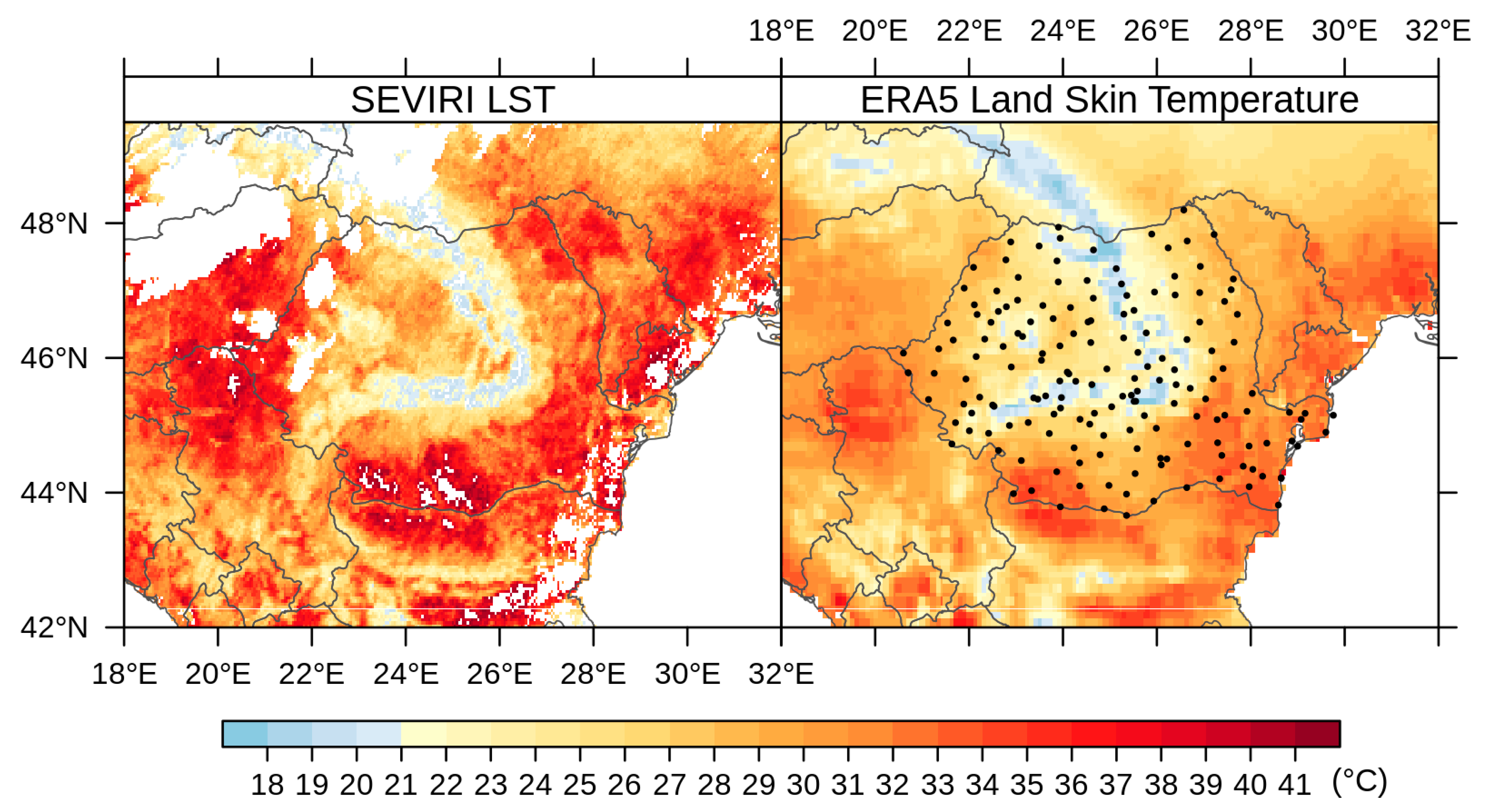
While the meteorological network of Romania is relatively efficient for climatological studies, as it captures all the geographical features at regional scale, some sub-regional or local patches are still scarcely covered with stations, e.g., Carpathian Mountains or extended plain areas (Figure 1, right panel). This work aims at developing and testing a fully formalized statistical methodology for obtaining complete series of SEVIRI LST hourly data. The methodology provides all weather estimations of gaps and it is based on a probabilistic model via modern regression models. The results have been demonstrated for the territory and immediate vicinity of Romania. Given the large volume of the data coupled with an enhanced accuracy derived by the use of auxiliary variables, we tested two categories of statistical methods of spatial estimation of air temperature, namely (1) a relatively simple multiple linear regression model, and (2) a more flexible alternative based on the general additive model [18,19,20,21,22,23,24].
Both approaches use a highly structured statistical calibration of the substitute temperature information source ERA5 Land skin temperature reanalysis data (ERA5ST) which is freely available at https://cds.climate.copernicus.eu/. The ultimate goal of this study is to develop a reliable and functional method for gap filling SEVIRI LST data using as co-variates the ERA5ST and additional easily accessible data (elevation, time, solar radiation).
2. Location and Data
The study area lies between 18°00′00″ and 32°00′00″E and 42°00′00″ and 49°30′00″N, covering Romania, but also parts of the neighboring countries (Figure 1). The analyzed region covers a total land area of 780,136 km2. The topography is fairly evenly distributed between lowlands, hilly areas and plateaus, and mountains (Carpathians) regions, with elevation ranging from sea level to 2544 m a.s.l.
This main input in this analysis is the hourly LST data set through 2016 and 2017, extracted from MSG-SEVIRI satellite images, which is an operational product of the Land Surface Analysis–Satellite Application Facility (LSA-SAF) [25]. The SEVIRI LST product is routinely available in HDF5 binary format in native geostationary projection, centered at 0° longitude and with a sampling distance of 3 km at the sub-satellite point [11]. Functions implemented in the GDAL (Geospatial Data Abstraction Library) were employed while transforming the SEVIRI LST data from geostationary to the WGS84 projection (Figure 1). Over the study area, the spatial resolution of the transformed SEVIRI LST data on a regular latitude/longitude grid is 0.042° × 0.042°, due to the pixel size increasing with latitude and longitude. GDAL is an open source library for manipulating geospatial data in both raster and vector formats [26]. In order to ensure the quality and homogeneity of the SEVIRI LST data and to remove possible sampling and processing errors, pixels with uncertain data have been removed according to the quality information accompanying the basic product, i.e., the Q_FLAGS band in the original HDF5 file [25].
Hourly skin temperature data extracted from the ERA5 Land (ERA5ST) reanalysis product was used as the main auxiliary variable in the gap-filling procedure used in this study. Both the ERA5ST reanalysis and the SEVIRI LST data refer to the same variable, namely the temperature at the level of the thin layer located at the interface between the terrestrial surface and the atmosphere [2] (Figure 1, right panel). The ERA5ST product available at a spatial resolution of 0.1° × 0.1° was spatially interpolated using the lapse rate method (MicroMet model) in order to harmonize the spatial resolution with the SEVIRI LST data set [27]. The quasi–physically based MicroMet model has been developed to produce high-resolution atmospheric variables required as input data in distributed terrestrial models over a wide variety of landscapes [28].
The elevation variable (ELEV) was extracted from the Shuttle Radar Topography Mission (SRTM) digital elevation model (DEM) [29]. The SRTM elevation data was upscaled to the SEVIRI LST spatial resolution by averaging the pixels coincident with each pixel of the SEVIRI LST data. The hourly CM SAF (The Satellite Application Facility on Climate Monitoring—www.cmsaf.eu) surface incoming shortwave radiation data (RAD) estimated from the MSG satellite images using Heliosat 2.1 model, was also used as a covariate for estimating the LST data [30]. The RAD product can be freely obtained for the period 1983–2017 from the CM SAF Web User Interface (https://wui.cmsaf.eu/safira/action/viewProduktSearch) at 0.05° × 0.05° spatial resolution, in a regular latitude/longitude grid. In the end, the ERA5 Land skin temperature, CMSAF solar radiation and DEM derived data were transformed into the geographical projection at the spatial resolution of the SEVIRI LST dataset, namelyWGS84, and respectively 0.042° × 0.042°.
3. Methods
The gap filling procedures performed in this study are based on a fully formalized statistical calibration of the ERA5 land skin temperature data (further denoted as ERA5) against LST, acknowledging various other additional covariates which might influence the LST–ERA5 relationship. The calibration model is estimated using the available LST locations. Once identified on training data, the calibration model can be used to fill the LST gaps by plugging in the ERA5 and other covariates into the model and evaluating the missing LST values within space-time slots. In order to evaluate the results, we have simulated the gap occurrence by creating random gaps at space-time slots where the LST value is actually known and compare the measurements to the model-based gap-filled LST data.
We have used two classes of regression models of different complexity and flexibility for the covariates calibration against LST, namely multiple linear regression (MLR) [21,24], and generalized additive model (GAM) [18,22,23]. The GAM approach was successful in many fields including meteorology and climatology in modeling potentially nonlinear relationships of unknown functional shape. It has to be noted that the shapes of the effects for different explanatory variables is recovered from data and does not rely on strong, unverifiable assumptions. We stress that we do not base our modeling on kriging or other methodology requiring stationarity (or even isotropy of the LST)— which would eventually not be satisfied. Instead, this GAM approach is based on penalized splines with roughness penalty inferred from the data via cross-validation [31,32,33]. The gap-filling performance has been tested using three models, namely one MLR (see Equation (1) below), and two GAM model versions (Equations (2) and (3)):
MLR:
where:
- is the LST value at spatial location s and time t.
- is the ERA5 value at spatial location s and time t.
- is the altitude at spatial location s.
- is the hour of time t.
- is the solar radiation at spatial location s and time t.
- is a normally distributed random error term,
- are unknown model coefficients to be inferred from the data (together with residual variance, ) via standard least squares algorithm.
From this specification, we can easily see that (1) is a standard multiple regression model that assumes linear relationship between LST and all the explanatory variables. This is simple both notionally and computationally but it is not clear a priori (from any kind of physical reasoning) that the assumed linear relationships really hold, at least approximately. If they would not hold, the LST estimates (and hence all LST gap-fills) would be biased and unreliable and could be improved by estimation in a more general regression model. To explore this issue, we formulate a more flexible GAM (generalized additive model) model analogue allowing for nonlinear (but smooth) relationship of LST to covariates.
GAM1:
where:
- are unknown smooth functions to be inferred from the data via penalized spline basis approximation and penalized likelihood maximization (with penalty coefficients estimated via generalized crossvalidation). Coefficients in the penalty term were estimated by generalized cross-validation procedure [34].
One can notice that the GAM1 model is a nonlinearity-allowing expansion of MLR. The model automatically adapts to smooth nonlinear trends. On the other hand, if the relationship would not differ from linear (which is not the case here), it would not insist on nonlinearity but reduce to essentially linear model. The model can be further expanded by introducing the effect of a distance between missing LST locations and the nearest non-missing location. The missing LST locations that are close to the boundary of the missing-LST area (e.g., to the boundary of a cloud) might be miscalculated by ERA5 since the exact cloud boundary could be somewhat blurred by both interpolation and finite spatial resolution of numerical weather models. To this end, we explored strength of the relationship between ERA5 and LST by distance from gap area edge. Figure 2 does indeed suggest that the existing distance effect should be rather local, in the sense that if the distance to the nearest non-missing point is larger than a given threshold, the adjustment for the distance from the missing-LST area boundary will not play any substantial role. Formalizing this finding, we are led to the following model GAM2—as an expansion of GAM1:
GAM2:
where:
- is the indicator function which assumes value of 1 if its argument is true and 0 if it is false. We use 50 km distance threshold after experimenting with different values.
One can remark that the complexity/generality/flexibility of the statistical models increases in the direction MLR, GAM1, GAM2 (the equivalent degrees of freedom for the three models are: 5 for MLR, 75 for GAM1, and 86 for GAM2).
Based on the fact that the hourly effect is significant in the models used in this study, we do not recommend to reduce them to hour-free version (e.g., to fit a simpler model on daily averages). Instead, when daily means are needed, we would really recommend to use hour model in hourly resolution and aggregate its output. It is worth mentioning that this can be done also for more complicated functionals of daily trajectory. For instance, based on the output of our fine-resolution GAM2 model, we might compute averages only over daylight hours, etc.
Taking into account the seasonal variability of the air temperature specific to the analyzed geographical area, it was decided that the regression models should be calibrated using subsets of data, for each month and year from the period analyzed (2016–2017).
The efficiency of the gap-filling approaches were evaluated for locations where artificial gaps were randomly created, i.e., 300 pixels with available data in each time slice of the original LST values, and the estimated LST values of these areas were compared with raw LST data (measurements). The distribution across different altitudinal steps of the artificial created gaps are directly related with the availability of the LST data (if LST raw data is available for one time slice on a certain area, then some of the 300 pixels are selected in that area). The mean absolute errors (MAE), root mean square errors (RMSE) and the Pearson’s correlation coefficient (CORR) were used as indicators for quantifying the accuracy of the gap-filling methods proposed.
4. Results
The seasonal percentage of missing LST SEVIRI data due to the cloud cover is shown in Figure 3. The missing data are plotted for each season by altitude steps: plains (below 300 m elevation), hills and plateaus (300–800 m elevation), and mountain (above 800 m elevation). The lowest rate of the missing data occurred during the summer (JJA) with an average of missing data below 50% in lowlands and in the hilly areas, whereas in the mountains regions the mean of missing data is above 50% even in summer. The thermal inversions can be depicted for the cold season (DJF), when the missing LST data in the mountains is slightly lower than in the plains and hilly areas, due to the lower cloud base. For the transition seasons (spring—MAM, and fall—SON), the average missing LST data due to cloud contamination is between 60% and 70%, excepting the MAM in the mountainous areas, when the cloudiness is 71.2%.
The statistical relationships between the analyzed variable and the selected predictors were tested by constructing scatterplots and computing the seasonal Pearson’s correlation coefficient. Figure 4 shows a strong linear statistical relationship between the LST and ERA5ST data sets, with correlation coefficients above 0.9, except for the winter months, from December to February (DJF). The lower correlation during the winter months is probably due to the frequent thermal inversions which alter the well-known physical relationships between LST and altitude. One can notice a good correlation between SEVIRI LST and the surface incoming shortwave radiation data (Table 1). The large spatial extension of the analysed area triggers a large variety of weather phenomena which can occur at the same time, such as thermal inversions, severe precipitation events and dry areas, or wind gusts and no wind patches that could determine a less steep LST gradient at an hourly time scale and the weakest correlation with elevation (ELEV).
For the GAM models, we first inspected extracted model components (like functions etc.) finding often quite strong nonlinearity which cannot be captured by standard linear models. This motivated us to compare carefully the gap filling results among different methods to see if the improved recovery of the functional relationships between LST and various explanatory variables does indeed lead to appreciable improvements in the gap-filling results.
In order to verify the performance of the three models, the seasonal accuracy indicators were computed (Table 2). The performance indicators computed for the GAM2 model are in all cases smaller than the GAM1 and MLR models, whether we refer to the MAE or the RMSE; these results are also confirmed by the calculation CORR, which is higher in all cases than the other two regression models. The estimates of the two GAMs models are superior to the MLR, regardless of the season and the accuracy indicator analysed. The performances of the three models were also investigated with scatterplots of modeled versus original SEVIRI LST data (Figure 5). The very good results obtained by the three models are also confirmed by the grouping of the points around the regression line. The closer value of the slopes to one computed between predictions and original data was also obtained by the GAM2 (the closer the slope is to one, the higher the similarity between the datasets). It has to be noted that better gap-filling performance of GAM2 when compared to GAM1 actually verifies the informal finding of Figure 2 that there is an important closeness to the cloud edge effect and that it can be used statistically to improve the gap-filling procedure in appreciable way.
Considering that the GAM2 model provides the closest estimates of the measured data according to all the criteria used, it was decided that this method should be applied to supplement the missing data LST series. Also, the very good results obtained from all the analyzed models suggest that the considered predictors satisfy the requirements for obtaining a complete LST data set. In order to obtain a gap-free data set of SEVIRI LST, 24 GAM2 models were calibrated for each year and month of the analyzed period (2016–2017).
The performances of the selected model (GAM2) were verified by comparing the estimated LST with the air temperature measured at several weather stations located in different topographic conditions of the analyzed area (Table 3). The hourly air temperature dataset was first quality-controlled and a homogenization method was applied to identify and correct any suspicious values [35]. The comparison was made only for the LST data estimated over the areas were no data was available within the raw SEVIRI LST dataset (Figure 6). The good agreement between the datasets indicate that the selected approach is appropriate for estimating LST data. Except for two situations, the Pearson’s correlation coefficient is above 0.7 regardless the season. The weakest correlation is observed at the Vârful Omu station which is located on a mountain peak, and therefore the corresponding LST value is retrieved from an area that contains valleys and different types of vegetation, while the air temperature is measured over an area with homogeneous land cover and topographic characteristics.
We also compared the raw and filled monthly averages of the LST data with the air temperature aggregated on monthly scale from the weather stations (Figure 7). The reconstructed LST values is almost equal to the raw LST values and slightly lower than the air temperature in the cold season. The poor match observed especially for the cold season at Vârful Omu station is because the LST data is estimated for a very heterogeneous area covering approximately 4.5 km2, while the ground-based measurements are representative only for the alpine conditions of the mountain.
Figure 8 shows the output of SEVIRI LST gap-filling over Romania in one summer hour. The visual investigation shows that the estimated LST values are coherent, regardless of the geographical region for which the filling was performed. The hourly original and completed SEVIRI LST data for the same day (20 July 2017) are shown in the Figures S1 and S2 from the Electronic Supplementary Material.
The benefit of using a complete SEVIRI LST hourly dataset is demonstrated by computing some synthesis maps illustrating the spatial distribution of the mean monthly minimum and maximum LST hardly available, which would remain unavailable without performing a gap-filling procedure at fine spatio-temporal resolution. The LST values decreases gradually from the lower areas (lowlands) to the high altitudes (Carpathian Mountains), were almost all the lowest minimum values are located (Figure 9). The thermal inversions clearly occur in January with the minimum values located in the Intra-Carpathian Depression, in the middle of the country where LST values are less than 18 °C. Also, the influences of the warm air coming from the Black Sea can be seen on the maps (south-eastern part of the country), were high LST values occurred in October, November, and January. The south-eastern part of Romania is warmer comparing to the rest of the country in October, November, December, and January, very likely due to the proximity of the Black Sea. The topography strongly biases the spatial distribution of the monthly maximum LST, the altitude imposing as a vertical thermal zonation factor (Figure 10). The thermal inversion phenomena are also observed in January, when certain areas located in the southern vicinity of the Carpathian Mountains are warmer (0–2 °C at 600–800 m a.s.l.) than the lower lands from the southern plain (−4 to 0 °C at 100–400 m a.s.l.).
Such maps are valuable because they could allow us to identify and analyze the areas affected by extreme weather events such as heat-waves and cold spells which constitute a major public health threat. The spatio-temporal estimation method can be evaluated at a given time on a grid at a spatial resolution similar to the input dataset. The aggregation of uncomplete LST data can facilitate the production of spatial and/or temporal statistics over locations and periods which otherwise would be very hard to obtain if no ground-based measurements are available.
5. Conclusions
This study addresses the need for improving the data coverage in areas with sparse meteorological information, embracing the combined use of climate reanalysis and remote sensing data. While satellite remote sensing is an efficient source for climate research increasingly used in recent decades, the lack of data due to cloudiness or technological barriers inherently occur in some area and periods. To the best of our knowledge, this is the first study which presents a statistical gap-filling approach of SEVIRI LST data demonstrated over a complex geographical area, i.e., Romania. The case study covers two years of hourly data, but the procedure can be applied to larger periods depending only on computing resources.
In order to select the appropriate gap-filling method, two categories of regression models were tested, namely the multiple linear regression model (MLR) and two models of general additive model (GAM) class. Three covariates were used for calibrating the MLR and GAM models: ERA5 Land skin temperature (ERA5ST), SRTM elevation (ELEV), and CMSAF short wave incoming solar radiation (RAD). Due to the low correlation between the LST and the best covariate (ERA5ST) found in the vicinity of the areas with gaps in the data, one more GAM model was tested in order to take into account the distance from missing LST pixels (GAM2). A very good correlation with the ERA5ST variable, i.e., Pearson’s correlation coefficient > 0.9 in spring, summer, and fall, and 0.859 in winter, was found by analyzing the resemblance between the predictand and the predictors. The seasonal difference is explained by the variation of the cloudiness conditions, including the cloud height and type, which strongly controls the correlation of LST with elevation in the case of SEVIRI, while the ERA5ST data do not take into account the cloud influence.
The models were calibrated and tested on monthly subsets, in order to eliminate the seasonality bias. For selecting the best gap-filling method, we randomly created artificial gaps in the raw SEVIRI LST product (300 pixels with available data in each time slice of the original LST data) at each time slice, for which the estimation procedure by the three methods was performed. The comparison between the estimated LST and the original LST values shows that GAM2 model provides the best results, hence this was used to fill the gaps from the analyzed remote sensing product.
Considering the fact that the best covariate (ERA5ST) has a global coverage and it is available at spatial resolution (0.1°) and temporal resolution (hourly) useful for many climatologic and environmental applications, with a wide temporal coverage (1981–present), the proposed approach could be also used to perform the gap-filling of other existing LST remote sensing products (MODIS, METOP, etc.). The data and statistical methods employed in this study are freely available and flexible to implement in order to achieve a complete series of the LST dataset over any geographical area.
Supplementary Materials
The following are available online at https://www.mdpi.com/2072-4292/12/9/1423/s1, Figure S1: Hourly SEVIRI LST raw data from 20 July 2017, Figure S2: Hourly SEVIRI LST gap-filled data from 20 July 2017.
Author Contributions
Conceptualization, A.D. and S.C.; Methodology, A.D., S.C. and M.B.; Software, A.D. and M.B.; Validation, A.D., M.B. and S.C.; Formal analysis, A.D. and S.C.; Data curation, A.D.; Writing—original draft preparation, A.D., S.C. and M.B. All authors have read and agreed to the published version of the manuscript.
Funding
This work was supported by a grant of Ministry of Research and Innovation, Romania, CNCS - UEFISCDI, project number PN-III-P1-1.1-PD-2016-1579, within PNCDI III. Partially supported by the long-term strategic development financing of the Institute of Computer Science (Czech Republic RVO 67985807).
Conflicts of Interest
The authors declare no conflict of interest.
References
- Copernicus Land Service. Copernicus Global Land Service Providing Bio-Geophysical Products of Global Land Surface. 2019. Available online: https://land.copernicus.eu/global/products/lst (accessed on 19 December 2019).
- ERA5-Land Data Documentation. 25 November 2019. Available online: https://confluence.ecmwf.int/display/CKB/ERA5-Land%3A+data+documentation (accessed on 4 April 2020).
- Apaydin, H.; Sonmez, F.K.; Yildirim, Y.E. Spatial interpolation techniques for climate data in the GAP region in Turkey. Clim. Res. 2004, 28, 31–40. [Google Scholar] [CrossRef] [Green Version]
- Henn, B.; Raleigh, M.S.; Fisher, A.; Lundquist, J.D. A Comparison of Methods for Filling Gaps in Hourly Near-Surface Air Temperature Data. J. Hydrometeorol. 2013, 14, 929–945. [Google Scholar] [CrossRef]
- Staub, B.; Hasler, A.; Noetzli, J.; Delaloye, R. Gap-Filling Algorithm for Ground Surface Temperature Data Measured in Permafrost and Periglacial Environments. Permafr. Periglac. Process. 2017, 28, 275–285. [Google Scholar] [CrossRef] [Green Version]
- Tardivo, G.; Berti, A. A Dynamic Method for Gap Filling in Daily Temperature Datasets. J. Appl. Meteorol. Climatol. 2012, 51, 1079–1086. [Google Scholar] [CrossRef]
- Martins, J.; Trigo, I.F.; Ghilain, N.; Jimenez, C.; Göttsche, F.-M.; Ermida, S.L.; Olesen, F.-S.; Gellens-Meulenberghs, F.; Arboleda, A. An All-Weather Land Surface Temperature Product Based on MSG/SEVIRI Observations. Remote Sens. 2019, 11, 3044. [Google Scholar] [CrossRef] [Green Version]
- Zhang, X.; Zhou, J.; Göttsche, F.M.; Zhan, W.; Liu, S.; Cao, R. A method based on temporal component decomposition for estimating 1-km all-weather land surface temperature by merging satellite thermal infrared and passive microwave observations. IEEE Trans. Geosci. Remote Sens. 2019, 57, 4670–4691. [Google Scholar] [CrossRef]
- Holmes, T.R.H.; Hain, C.R.; Anderson, M.C.; Crow, W.T. Cloud tolerance of remote-sensing technologies to measure land surface temperature. Hydrol. Earth Syst. Sci. 2016, 20. [Google Scholar] [CrossRef] [Green Version]
- Li, X.; Zhou, Y.; Asrar, G.R.; Zhu, Z. Creating a seamless 1 km resolution daily land surface temperature dataset for urban and surrounding areas in the conterminous United States. Remote Sens. Environ. 2018, 206, 84–97. [Google Scholar] [CrossRef]
- Land SAF Project Team. Product User Manual Land Surface Temperature (LST); PRODUCTS: LSA-001 (MLST), LSA-050 (MLST-R), LSA-003 (DLST), LSA-002 (ELST); Land SAF Project Team: Lisabon, Portugal, 2018. [Google Scholar]
- Coops, N.C.; Duro, D.C.; Wulder, M.A.; Han, T. Estimating afternoon MODIS land surface temperatures (LST) based on morning MODIS overpass, location and elevation information. Int. J. Remote Sens. 2007, 28, 2391–2396. [Google Scholar] [CrossRef]
- Duan, S.-B.; Li, Z.-L.; Leng, P. A framework for the retrieval of all-weather land surface temperature at a high spatial resolution from polar-orbiting thermal infrared and passive microwave data. Remote Sens. Environ. 2017, 195, 107–117. [Google Scholar] [CrossRef]
- Neteler, M. Estimating daily land surface temperatures in mountainous environments by reconstructed MODIS LST data. Remote Sens. 2010, 2, 333–351. [Google Scholar] [CrossRef] [Green Version]
- Kilibarda, M.; Hengl, T.; Heuvelink, G.B.M.; Gräler, B.; Pebesma, E.; Tadić, M.P.; Bajat, B. Spatio-temporal interpolation of daily temperatures for global land areas at 1 km resolution. J. Geophys. Res. Atmos. 2014, 119, 2294–2313. [Google Scholar] [CrossRef] [Green Version]
- Weiss, D.J.; Atkinson, P.M.; Bhatt, S.; Mappin, B.; Hay, S.I.; Gething, P.W. An effective approach for gap-filling continental scale remotely sensed time-series. ISPRS J. Photogramm. Remote Sens. 2014, 98, 106–118. [Google Scholar] [CrossRef] [PubMed] [Green Version]
- Metz, M.; Andreo, V.; Neteler, M. A new fully gap-free time series of land surface temperature from MODIS LST data. Remote Sens. 2017, 9, 1333. [Google Scholar] [CrossRef] [Green Version]
- Aalto, J.; Pirinen, P.; Heikkinen, J.; Venäläinen, A. Spatial interpolation of monthly climate data for Finland: Comparing the performance of kriging and generalized additive models. Theor. Appl. Climatol. 2013, 112, 99–111. [Google Scholar] [CrossRef]
- Ruiz-Álvarez, M.; Alonso-Sarría, F.; Gomariz-Castillo, F. Interpolation of Instantaneous Air Temperature Using Geographical and MODIS Derived Variables with Machine Learning Techniques. ISPRS Int. J. Geo-Inf. 2019, 8, 382. [Google Scholar] [CrossRef] [Green Version]
- Szymanowski, M.; Kryza, M.; Spallek, W. Regression-based air temperature spatial prediction models: An example from Poland. Meteorol. Z. 2013, 22, 577–585. [Google Scholar] [CrossRef]
- Rawlings, J.O.; Pantula, S.G.; Dickey, D.A. Applied Regression Analysis: A Research Tool; Springer: Berlin/Heidelberg, Germany, 1998. [Google Scholar]
- Wood, S.N. Generalized Additive Models: An Introduction with R.; Chapman and Hall/CRC: Boca Raton, FL, USA, 2017. [Google Scholar]
- Hastie, T.J.; Tibshirani, R.J. Generalized Additive Models; Chapman & Hall/CRC: Boca Raton, FL, USA, 1990. [Google Scholar]
- Searle, S.R.; Gruber, M.H.J. Linear Models; John Wiley & Sons: Hoboken, NJ, USA, 2016. [Google Scholar]
- SAF LSA, Eumetsat LSA SAF Land Surface Analysis. 2019. Available online: https://landsaf.ipma.pt/en/ (accessed on 20 December 2019).
- GDAL/OGR Contributors, GDAL/OGR Geospatial Data Abstraction Software Library. 2019. Available online: https://gdal.org (accessed on 19 December 2019).
- Liston, G.E.; Elder, K. A meteorological distribution system for high-resolution terrestrial modeling (MicroMet). J. Hydrometeorol. 2006, 7, 217–234. [Google Scholar] [CrossRef] [Green Version]
- Gascoin, S.; Lhermitte, S.; Kinnard, C.; Bortels, K.; Liston, G.E. Wind effects on snow cover in Pascua-Lama, Dry Andes of Chile. Adv. Water Resour. 2013, 55, 25–39. [Google Scholar] [CrossRef] [Green Version]
- Jarvis, A.; Reuter, H.I.; Nelson, A.; Guevara, E. Hole-Filled Seamless SRTM Data V4; International Centre for Tropical Agriculture (CIAT): Cali, Colombia, 2008. [Google Scholar]
- Pfeifroth, U.; Kothe, S.; Müller, R.; Trentmann, J.; Hollmann, R.; Fuchs, P.; Werscheck, M. Surface Radiation Data Set—Heliosat (SARAH)—Edition 2, Satellite Application Facility on Climate Monitoring; Satellite Application Facility on Climate Monitoring (CM SAF): Offenbach, Germany, 2017. [Google Scholar]
- Eilers, P.H.C.; Marx, B.D. Flexible smoothing with B-splines and penalties. Stat. Sci. 1996, 11, 89–102. [Google Scholar] [CrossRef]
- Wood, S.N.; Pya, N.; Säfken, B. Smoothing parameter and model selection for general smooth models. J. Am. Stat. Assoc. 2016, 111, 1548–1563. [Google Scholar] [CrossRef]
- De Boor, C.; de Boor, C.; Mathématicien, E.-U.; de Boor, C.; de Boor, C. A Practical Guide to Splines; Springer: Berlin/Heidelberg, Germany, 1978; Volume 27. [Google Scholar]
- Wood, S.N. Fast stable direct fitting and smoothness selection for generalized additive models. J. R. Stat. Soc. Ser. B (Stat. Methodol.) 2008, 70, 495–518. [Google Scholar] [CrossRef] [Green Version]
- Dumitrescu, A.; Cheval, S.; Guijarro, J.A. Homogenization of a combined hourly air temperature dataset over Romania. Int. J. Climatol. 2020, 40, 2599–2608. [Google Scholar] [CrossRef]
Figure 1.
SEVIRI LST (left) and ERA5 Land Skin temperature (right): 2017-08-25 09 UTC. The black dots from the right panel are the weather stations of the Romanian National Meteorological Administration.
Figure 1.
SEVIRI LST (left) and ERA5 Land Skin temperature (right): 2017-08-25 09 UTC. The black dots from the right panel are the weather stations of the Romanian National Meteorological Administration.

Figure 2.
Pearson correlation coefficient (SEVIRI LST vs. ERA5 Land skin temperature) computed on different distances from the LST missing data areas.
Figure 2.
Pearson correlation coefficient (SEVIRI LST vs. ERA5 Land skin temperature) computed on different distances from the LST missing data areas.

Figure 3.
Seasonal density plots of the percentage of the missing LST data computed for each pixel by altitudinal steps. The vertical black lines represent the average percentages of the missing values for each subset of the data.
Figure 3.
Seasonal density plots of the percentage of the missing LST data computed for each pixel by altitudinal steps. The vertical black lines represent the average percentages of the missing values for each subset of the data.

Figure 4.
SEVIRI LST vs. ERA5ST (2016–2017), based on randomly selected pixels (300/h). Blue lines shown on the plot are the best fit lines of the linear model between the two analyzed datasets.
Figure 4.
SEVIRI LST vs. ERA5ST (2016–2017), based on randomly selected pixels (300/h). Blue lines shown on the plot are the best fit lines of the linear model between the two analyzed datasets.

Figure 5.
Seasonal scatterplots: hourly raw SEVIRI LST data vs. hourly estimated SEVIRI LST (2016–2017), based on randomly selected pixels (300/h). Red lines show the best fit lines of the linear model between the two analyzed datasets, and the grey lines are the perfect fit linear models.
Figure 5.
Seasonal scatterplots: hourly raw SEVIRI LST data vs. hourly estimated SEVIRI LST (2016–2017), based on randomly selected pixels (300/h). Red lines show the best fit lines of the linear model between the two analyzed datasets, and the grey lines are the perfect fit linear models.

Figure 6.
Seasonal scatterplots between the hourly estimated LST and hourly air temperature obtained from five meteorological stations (2016–2017). Red lines represent the best fit lines of the linear model between the two analyzed datasets, and the grey lines are the perfect fit linear models.
Figure 6.
Seasonal scatterplots between the hourly estimated LST and hourly air temperature obtained from five meteorological stations (2016–2017). Red lines represent the best fit lines of the linear model between the two analyzed datasets, and the grey lines are the perfect fit linear models.

Figure 7.
Time series plots of monthly averages LST data (raw and filled) and air temperature extracted at five weather stations location from 2016 to 2017.
Figure 7.
Time series plots of monthly averages LST data (raw and filled) and air temperature extracted at five weather stations location from 2016 to 2017.

Figure 8.
SEVIRI LST (° C) data from July 20, 2017, 4:00 pm UTC: original image (left) and completed data (right).
Figure 8.
SEVIRI LST (° C) data from July 20, 2017, 4:00 pm UTC: original image (left) and completed data (right).

Figure 9.
Monthly mean minimum LST (°C) from 2016 to 2017.

Figure 10.
Monthly mean maximum LST (°C) from 2016 to 2017.


Table 1.
Pearson’s correlation coefficients between SEVIRI LST and selected covariates: elevation (ELEV), surface incoming shortwave radiation (RAD), and ERA5 Land skin temperature (ERA5ST).
Table 1.
Pearson’s correlation coefficients between SEVIRI LST and selected covariates: elevation (ELEV), surface incoming shortwave radiation (RAD), and ERA5 Land skin temperature (ERA5ST).
| Covariate | DJF | MAM | JJA | SON |
|---|---|---|---|---|
| ELEV | −0.140 | −0.234 | −0.320 | −0.200 |
| RAD | 0.598 | 0.820 | 0.817 | 0.736 |
| ERA5ST | 0.859 | 0.926 | 0.925 | 0.936 |
Table 2.
Seasonal mean values of absolute mean errors (MAE), root mean square errors (RMSE), and Pearson’s correlation coefficients (CORR) (2016–2017).
Table 2.
Seasonal mean values of absolute mean errors (MAE), root mean square errors (RMSE), and Pearson’s correlation coefficients (CORR) (2016–2017).
| Model | Season | MAE | RMSE | CORR |
|---|---|---|---|---|
| MLR | DJF | 2.795 | 3.745 | 0.888 |
| GAM1 | DJF | 2.583 | 3.511 | 0.902 |
| GAM2 | DJF | 2.493 | 3.351 | 0.911 |
| MLR | MAM | 2.173 | 2.900 | 0.950 |
| GAM1 | MAM | 1.979 | 2.696 | 0.957 |
| GAM2 | MAM | 1.926 | 2.603 | 0.960 |
| MLR | JJA | 1.934 | 2.491 | 0.953 |
| GAM1 | JJA | 1.811 | 2.351 | 0.958 |
| GAM2 | JJA | 1.796 | 2.328 | 0.959 |
| MLR | SON | 2.117 | 2.799 | 0.958 |
| GAM1 | SON | 1.900 | 2.564 | 0.965 |
| GAM2 | SON | 1.848 | 2.462 | 0.968 |
Table 3.
Metadata of the weather stations from which the air temperature data was obtained.
| Name | Longitude East (Decimal Degrees) | Latitude North (Decimal Degrees) | Elevation above Sea Level (m) |
|---|---|---|---|
| București Filaret | 26.0938 | 44.4121 | 82 |
| Câmpina | 25.7334 | 45.1437 | 461 |
| Mangalia | 28.5874 | 43.8161 | 1 |
| Miercurea Ciuc | 25.7726 | 46.3713 | 667 |
| Vârful Omu | 25.4567 | 45.4458 | 2506 |
© 2020 by the authors. Licensee MDPI, Basel, Switzerland. This article is an open access article distributed under the terms and conditions of the Creative Commons Attribution (CC BY) license (http://creativecommons.org/licenses/by/4.0/).
Share and Cite
MDPI and ACS Style
Dumitrescu, A.; Brabec, M.; Cheval, S. Statistical Gap-Filling of SEVIRI Land Surface Temperature. Remote Sens. 2020, 12, 1423. https://doi.org/10.3390/rs12091423
AMA Style
Dumitrescu A, Brabec M, Cheval S. Statistical Gap-Filling of SEVIRI Land Surface Temperature. Remote Sensing. 2020; 12(9):1423. https://doi.org/10.3390/rs12091423
Chicago/Turabian StyleDumitrescu, Alexandru, Marek Brabec, and Sorin Cheval. 2020. "Statistical Gap-Filling of SEVIRI Land Surface Temperature" Remote Sensing 12, no. 9: 1423. https://doi.org/10.3390/rs12091423
Note that from the first issue of 2016, this journal uses article numbers instead of page numbers. See further details here.