Article

Cluster Low-Streams Regression Method for Hyperspectral Radiative Transfer Computations: Cases of O2 A- and CO2 Bands

by
Ana del Águila
1,*,
Dmitry S. Efremenko
1,
Víctor Molina García
1 and
Michael Yu. Kataev
2
1
Remote Sensing Technology Institute, German Aerospace Center (DLR), 82234 Oberpfaffenhofen, Germany
2
Department of Control Systems, Tomsk State University of Control Systems and Radioelectronics, Tomsk 634050, Russia
*
Author to whom correspondence should be addressed.
Remote Sens. 2020, 12(8), 1250; https://doi.org/10.3390/rs12081250
Submission received: 19 March 2020 / Revised: 7 April 2020 / Accepted: 10 April 2020 / Published: 15 April 2020

Abstract

:
Current atmospheric composition sensors provide a large amount of high spectral resolution data. The accurate processing of this data employs time-consuming line-by-line (LBL) radiative transfer models (RTMs). In this paper, we describe a method to accelerate hyperspectral radiative transfer models based on the clustering of the spectral radiances computed with a low-stream RTM and the regression analysis performed for the low-stream and multi-stream RTMs within each cluster. This approach, which we refer to as the Cluster Low-Streams Regression (CLSR) method, is applied for computing the radiance spectra in the O2 A-band at 760 nm and the CO2 band at 1610 nm for five atmospheric scenarios. The CLSR method is also compared with the principal component analysis (PCA)-based RTM, showing an improvement in terms of accuracy and computational performance over PCA-based RTMs. As low-stream models, the two-stream and the single-scattering RTMs are considered. We show that the error of this approach is modulated by the optical thickness of the atmosphere. Nevertheless, the CLSR method provides a performance enhancement of almost two orders of magnitude compared to the LBL model, while the error of the technique is below 0.1% for both bands.

Graphical Abstract

1. Introduction

Radiative transfer models (RTM) are a key part of the remote sensing algorithms, which are used to retrieve atmospheric parameters from Earth observation data. The new atmospheric composition sensors with high spatial and spectral resolution require accurate and efficient computational algorithms. An accurate method to simulate spectral radiances in the absorption bands is the line-by-line (LBL) approach [1]. However, due to the high spectral variability of the gas absorption coefficient k in the absorption bands, the LBL-approach is very time-consuming because it requires up to several thousands of monochromatic computations per absorption band. In this regard, specifically designed hyperspectral RTMs are required. They reduce the number of monochromatic computations considerably without compromising accuracy. The basic idea behind the hyperspectral RTMs is to get rid of redundancies in hyperspectral data. This principle can be traced back to Ambartsumian [2], who noted that the transmission within a spectral interval does not depend on the LBL variation of k, but rather on the distribution of values of k within the spectral interval. This idea was used in the k-distribution method [3,4,5,6], in which the wavelengths are grouped into a smaller number of bins with similar values of k, and the LBL calculations are replaced by a smaller set of radiative transfer simulations. In [7,8], the transmission function for a given spectral interval is fitted by a sum of exponentials, while the corresponding fitting coefficients are computed from a reduced number of monochromatic computations. A similar approach is described in Moncet et al. [9], where the fitting weights and the most representative wavelengths are chosen appropriately.
The state-of-the-art hyperspectral RTMs employ dimensionality reduction techniques such as principal component analysis (PCA). In [10,11], PCA is applied to the spectral radiance data to establish a set of empirical orthogonal functions (EOFs), so that an arbitrary spectrum at full spectral resolution can be reconstructed as a weighted sum of EOFs. The weights are found by performing monochromatic simulations at a reduced number of wavelengths. To accelerate the computations in the O2 A-band, Natraj et al. [12] proposed a fundamentally different PCA-based radiative transfer model, in which the dimensionality of the optical properties data is reduced. A two-stream radiative transfer model was used as an approximate model, and the dependency of the corresponding correction factor on the optical parameters was modeled by a second-order Taylor expansion about the mean value of the optical parameters in the reduced optical data space. This approach was extended to other dimensionality reduction techniques [13] and spectral ranges [14,15,16]; moreover, it was implemented in conjunction with PCA for spectral radiances [17] and with the k-distribution method [18]. The errors of these approaches are usually below 0.1% for the spectral radiances, while the performance enhancement may reach several orders of magnitude depending on the spectral region and the required level of accuracy.
In Efremenko et al. [19] it was shown that, after parallelizing the PCA-based RTM computations, as much as half of the computational time is due to the PCA itself; consequently, according to Amdahl’s Law [20], no further acceleration of a PCA-based RTM is possible. In this regard, it is of great interest to develop acceleration techniques for hyperspectral RTM computations that do not exploit PCA. A possible candidate, which deserves this purpose, is the low streams interpolation method proposed by O’Dell [21]. In this method, (i) each spectral point is assigned to a specific bin according to the values of the gas optical depth, (ii) an approximate two-stream model is used to compute the radiances at all spectral points, and (iii) the two-stream radiances are corrected to the multi-stream radiances by calling a multi-stream model only once for each bin. In this paper, we propose the so-called Cluster Low-Streams Regression (CLSR) method, in which (i) wavelengths are grouped according to the radiance values obtained with the approximate model (rather than the optical properties), and (ii) the single-scattering and the two-stream models are used as approximate models. The CLSR method is tested against the PCA-based RTM for the O2 A-band at 760 nm and the weak CO2 band at 1610 nm. These spectral bands are of great interest for retrieving aerosol and cloud parameters [22], as well as CO2 concentrations [23].
The paper is organized as follows. In Section 2, the methodology is presented, including the descriptions of the PCA-based RTM adopted in our research and the CLSR method. In Section 3, the accuracy and efficiency of the CLSR method for several atmospheric scenarios in the O2 A- and weak CO2 absorption bands are analyzed and compared with the PCA-based RTM. In addition, the accuracy of the radiance spectra convolved with the slit functions corresponding to GOME-2 [24], TROPOMI on board Sentinel 5-P [25] and GOSAT [26] instruments is examined. The paper concludes with a summary.

2. Methodology

2.1. Reference Radiative Transfer Model

As a reference RTM, the scalar method of discrete ordinates with matrix exponential (DOME) [27] is used. The model is supplied with the left eigenvector approach [28,29,30] based on the scaling transformation [31,32]. In this method, the number of discrete ordinates (streams) in the polar hemisphere N do controls the computational time and accuracy. The model is called multi-stream (MS) when N do 2 and low-stream (LS) otherwise. Specifically, the case N do = 1 is the two-stream model. The simplest RTM is the single-scattering model, which solves the radiative transfer equation neglecting the integral term [33].
The gaseous absorptions for the O2 A- and CO2 bands are computed with the LBL model Py4CAtS [34], while the gas absorption cross-sections are taken from the HITRAN 2016 database [35]. The uncertainties in the spectroscopic parameters are not considered because their role is irrelevant for this study [36]. Continuum (also referred to as collision-induced absorption (CIA) [37,38]) contributions to molecular absorption are not taken into account. We note that the CIA process gives a broad and smooth contribution [39] and hence, does not impose difficulties for the regression techniques considered in this study.

2.2. Study Cases

We consider the reflected spectral radiance at the top of the atmosphere (TOA). In our simulations, the atmosphere is discretized into 35 layers with a step of 1 km between 0 and 25 km, and a step of 2.5 km between 25 km and 50 km. We assume a Lambertian surface with an albedo of 0.3. The solar zenith angle, the viewing zenith angle and the relative azimuth angle are 45°, 35° and 90°, respectively.
In the O2 A-band the spectral sampling is 0.001 nm in the spectral range 755–775 nm, while in the CO2 band the spectral sampling is 0.0015 nm in the spectral interval 1590–1620 nm. Thus, on each band, 20,000 spectral points are considered. The Rayleigh cross-sections and depolarization ratios are computed as in [40], while the pressure and temperature profiles correspond to the US standard model atmosphere [41]. The computations are performed for the unit solar irradiance at the TOA.
We define 5 atmospheric scenarios: ‘Clear sky’, ‘Aerosol 1’, ‘Aerosol 2’, ‘Cloud 1’ and ‘Cloud 2’. The ‘Clear sky’ scenario corresponds to an atmosphere without clouds and aerosols. In the ‘Aerosol 1’ and ‘Aerosol 2’ scenarios, the atmosphere contains the clean continental and the polluted continental aerosols taken from the OPAC database [42], respectively. The aerosol optical depths at the middle of the absorption bands are shown in Table 1. In the ‘Cloud 1’ and ‘Cloud 2’ scenarios, a continental clean cumulus cloud with a modified Gamma size distribution [42,43]:
p ( a ) a α exp α γ a a mod γ ,
is considered. The size distribution parameters are a mod = 4.8 µm, α = 5 and γ = 2.16 , the droplet size ranges between 0.02 and 50.0 µm, and the cloud optical depths are τ = 10 (‘Cloud 1’) and τ = 20 (‘Cloud 2’). In both cases, the cloud-top height is 5 km and the cloud geometrical thickness is 1 km.
The number of streams considered for the multi-stream model is the same for all scenarios. We might need a different number of streams for different scenarios, but in order to simplify and ensure convergence of relative errors for all cases, we use 32 streams.

2.3. PCA-Based RTM

Since a PCA-based RTM can be implemented in several ways (e.g., [12,13,15,16,17,44,45]), we describe below the main features of the PCA-based RTM used in this paper. The idea of the method is to refine the two-stream solution by a correction function estimated in the reduced space of the optical properties. Considering a discretization of the atmosphere in L layers, we define a 2 L -dimensional vector x w for each wavelength { λ w } w = 1 W , by
x w T = ln τ 1 ( λ w ) , , ln τ L ( λ w ) , ln ω 1 ( λ w ) , , ln ω L ( λ w ) ,
where τ k and ω k are the optical thickness and the single-scattering albedo of the k-th layer, respectively. Thus, the vector x w encapsulates the wavelength variability of the optical parameters, which are the input parameters of the radiative transfer code. By applying PCA, a M-dimensional subspace is found which is spanned by a set of linear independent vectors (empirical orthogonal functions) { q k } k = 1 M such that the centered (mean-removed) data x w x ¯ lie mainly on this subspace, i.e.,
x w x ¯ + k = 1 M y w k q k , w = 1 , , W ,
where y w k are the principal component (PC) scores.
Following Natraj et al. [12], we introduce a correction function
f ( x w ) = ln I MS ( x w ) I LS ( x w ) ,
where I LS ( x w ) is the radiance provided by the low-stream RTM, and I MS ( x w ) is the radiance simulated by the multi-stream model. Setting Δ x w = k = 1 M y w k q k , we consider a second-order Taylor expansion of f ( x w ) around x ¯ in the direction Δ x w . Approximating the directional derivatives with central differences (see [13,17] for mathematical details) we obtain
f ( x w ) f ( x ¯ ) + 1 2 k = 1 M [ f ( x ¯ + q k ) f ( x ¯ q k ) ] y w k + 1 2 k = 1 M [ f ( x ¯ + q k ) 2 f ( x ¯ ) + f ( x ¯ q k ) ] y w k 2 .
Please note, since M < 2 L (and in practice, M 2 L ), the estimation of the correction function in the reduced data space is much faster than in the original space. Also note that the total number of calls of the multi-stream RTM is 2 M + 1 . Once f ( x w ) is computed, the low-stream radiances can be converted into the multi-stream radiances by using Equation (3). Finally, the predicted multi-stream radiance I ˜ MS can be expressed as follows:
I ˜ MS = I LS exp [ f ( x w ) ] .
In del Águila et al. [17], it was shown that a higher order expansion of f ( x w ) in Equation (4) does not substantially improve the accuracy of the solution. In our simulations, an appropriate value for M is found iteratively, i.e., M is increased until the approximation error is sufficiently small.

2.4. Regression Relationship between Multi-Stream and Low-Stream Models

The LBL computations can be accelerated by finding a regression relationship between the multi-stream radiances and the optical parameters. In O’Dell [21], the correction function of the low-stream radiance as a function of the gas optical thickness τ gas , i.e., the relative error
f ( τ gas ) = I LS ( τ gas ) I MS ( τ gas ) I MS ( τ gas ) ,
was analyzed (Figure 1). The idea is to compute f ( τ gas ) at certain values of τ gas , and then to use a regression model for computing f ( τ gas ) at the remaining values of τ gas . However, for the present application, such an approach has two major drawbacks:
1.
the dependence of f ( τ gas ) on τ gas is non-linear and, therefore, the application of the regression model requires a binning of the τ gas values;
2.
in a mathematical sense, f ( τ gas ) is not a function (for a value of τ gas , there are several values of f ( τ gas ) ) and therefore, even for a fine binning, the regression model will be not accurate.
To overcome these drawbacks, O’Dell [21] devised a regression model based on the so-called adjusted gas optical thickness, defined as the gas optical thickness from the TOA down to the layer in the atmosphere where the scattering optical depth equals some critical value.
A similar idea, which we exploit in the following, is to use a regression model for the radiances computed by a low-stream RTM rather than in the τ gas -space. Figure 2 shows a comparison between the multi- and low-stream radiances for the ‘Aerosol 2’ scenario. Although the errors of the low-stream RTM are significant (e.g., they may reach 200%), the low- and multi-stream radiances have a similar spectral behaviour. Moreover, as shown in Figure 3, the dependence between the low- and multi-stream radiances is almost linear. In this respect, it seems reasonable to cluster the spectral points according to the radiance values computed with a low-stream RTM (rather than according to the optical properties) and to establish a regression model between the low- and multi-stream radiances within each cluster. In order to decrease the errors of the regression estimates, an additional wavelength-dependent parameter will be included in the regression model: the direct transmittance T.

2.5. Cluster Low-Streams Regression Method

The Cluster Low-Streams Regression (CLSR) method can be formulated as follows.
1.
Consider a high-resolution spectrum { I LS ( λ i ) } i = 1 N computed at N spectral points { λ i } i = 1 N by means of a low-stream RTM.
2.
Sort the radiance set { I LS ( λ i ) } i = 1 N in ascending order, and let { I ^ LS , i } i = 1 N , with I ^ LS , i I ^ LS , i + 1 , be the sorted radiance set (Figure 4a).
3.
Consider C clusters in { I ^ LS , i } i = 1 N with N C = N / C radiance points (Figure 4b), and let the c cluster be defined by the radiance set { I ^ LS , i c } i = 1 N C for c = 1 , , C .
4.
Select n equidistant radiance points in the c cluster, i.e., { I ¯ LS , q c } q = 1 n , and for the corresponding wavelengths compute the multi-stream radiances { I ¯ MS , q c } q = 1 n (Figure 4c).
5.
Assume that in each cluster c we have the linear relationship
I ^ MS , i c = α c T ^ i c + β c I ^ LS , i c + γ c , i = 1 , , N C ,
where α c , β c and γ c are the regression coefficients of the c-th cluster, and T ^ is the corresponding direct transmittance.
6.
Compute the regression coefficients α c , β c and γ c as a solution to the least square problem
α c , β c , γ c = arg min α c , β c , γ c q = 1 n I ¯ MS , q c α c T ¯ q c + β c I ¯ LS , q c + γ c 2 .
7.
Use the values of ( α c , β c , γ c ) found in the previous step to restore the multi-stream radiances { I ˜ MS , i } i = 1 N for all the spectral points according to Equation (6) (Figure 4d).
Here, the “hat” notation I ^ refers to the sorted radiances, the “bar” notation I ¯ refers to the equidistant radiances entering the regression model, and the “tilde” notation I ˜ refers to the predicted radiances. Please note that the total number of regression points, and thus the number of calls of the multi-stream model, is n C .

2.6. Efficiency and Computational Performance Estimation

To estimate the accuracy of the acceleration techniques, we consider the residual error for the radiance at each spectral point λ i :
Δ I res , i = I ˜ MS , i I MS , i I MS cont · 100 ,
where I ˜ MS , i is the predicted radiance calculated with either the PCA-based RTM (cf. Equation (5)) or the CLSR method (cf. Equation (6)), while I MS cont is the radiance without absorption (i.e., the continuum radiance, which is used to avoid radiance values close to zero in the denominator of Equation (8), when strong gas absorption is present [15]). The mean relative error is computed as follows:
ε = i = 1 N Δ I res , i N .
Additionally, the median and interquartile range (IQR) of the residual are computed. Essentially, these parameters serve as robust metrics to evaluate the variability of the residuals in the corresponding spectral band, thereby with a lower sensitivity to single outliers [16].
To estimate the performance enhancement, we define the speedup factor as the ratio between the computational time of a multi-stream LBL calculation to that of a certain acceleration technique. To exclude the hardware-related factors from our analysis, we estimate the speedup factor for the PCA-based RTM as [16]
S PCA = t MS × N t LS × N + t PCA + ( 2 M + 1 ) ( t MS + t LS ) ,
where t MS and t LS are the computational times for a single monochromatic calculation corresponding to the multi- and low-stream RTMs, respectively, while t PCA is the computational time of the PCA. Thus, the numerator in Equation (10) is the time required for the LBL computations. Please note the PCA-based RTM requires 2 M + 1 calls to the multi-stream model.
The speedup factor for the CLSR method is defined by
S CLSR = t MS × N t LS × N + t LSM × C + t MS × n × C ,
where t LSM is the computational time needed for the least-squares method according to Equation (7). Recall that the total number of regression points and the corresponding calls of the multi-stream model is n C .

3. Results and Discussion

3.1. Performance of the Low- and Multi-Streams Models

In this section, we assess the performance of the low- and multi-stream RTMs before applying the acceleration techniques. The spectral radiances for three atmospheric scenarios (‘Clear sky’, ‘Cloud 1’ and ‘Cloud 2’) are illustrated in Figure 5.
Table 2 and Table 3 provide the mean relative errors of the low-stream RTMs with respect to the multi-stream RTM for the O2 A- and CO2 absorption bands, respectively. Table 4 shows the computational performance for a different number of discrete ordinates N do . The results show that (i) the relative errors of the single-scattering model are higher than those of the two-stream model, (ii) the relative error increases as the optical thickness of the atmosphere increases, and (iii) the speedup factors of the single-scattering model are considerably higher than those of the two-stream model.

3.2. Acceleration Techniques: Accuracy Evaluation

3.2.1. Spectral Residuals

The residuals (cf. Equation (8)) are computed for (i) different numbers of principal components in the case of the PCA-based RTM, and (ii) different numbers of regression points per cluster in the case of the CLSR method. Figure 6 shows these residuals for the ‘Cloud 2’ and the ‘Aerosol 2’ scenarios.
From Figure 6 the following conclusions can be drawn.
1.
The residuals decrease when increasing the number of PCs and regression points.
2.
The interquartile range for the CLSR method is substantially reduced when switching from 1–2 to 3 regression points for the CO2 band, and from 3 to 4 regression points for the O2 A-band.
3.
In both spectral bands, the interquartile range for the PCA-based RTM decreases gradually with the number of principal components.
4.
The residuals in the O2 A-band are systematically higher than those in the CO2 band. This behaviour is more pronounced when the gas optical thickness is large, thus resulting in larger discrepancies for the PCA-based RTM and almost negligible discrepancies for the CLSR approach.
5.
In the O2 A-band, the median values of the residuals Equation (8) are higher than 2%. The median values remain almost constant with the number of principal components and regression points. However, the median values as well as the interquartile range for the PCA method are generally higher than those of the CLSR method. This trend remains coherent using the single-scattering RTM instead of the two-stream RTM, although the residuals are substantially higher for the PCA-based RTM.

3.2.2. Estimation of the Required Parameters for the Acceleration Techniques

In order to select the optimal number of PCs, we compute the explained variance ratio of the optical data, which accounts for the variance associated with a given number of PCs. The results in Figure 7 show that in all scenarios almost 99% of the optical data variance can be explained within the first four PCs. Moreover, from Figure 6a we can infer that (i) the convergence of the two-stream radiances is reached for 4-5 PCs, while (ii) the convergence of the single-scattering radiances requires 4-7 PCs (Figure 6b).
To select the number of clusters and regression points for the CLSR method, we estimate the mean error (cf. Equation (9)). As an example, we illustrate in Figure 8 the mean errors for the ‘Aerosol 2’ scenario. The results show that 4–5 clusters and 3–5 regression points guarantee a small mean error.

3.2.3. Accuracy of the CLSR and PCA-Based Methods

In this section, we assess the accuracy of the PCA-based and CLSR methods. The residuals (Equation (8)) and interquartile ranges corresponding to the PCA-based and CLSR methods, as well as for the two-stream and single-scattering models, are shown in Figure 9.
The results can be summarized as follows:
1.
For both low-stream models and cloudy scenarios, (i) the residuals of the PCA-based method in the O2 A-band are substantially larger than those of the CLSR method (on average, for the two-stream model in the O2 A-band, the residuals are above 1% for the PCA-based method and below 0.01% for the CLSR method), while (ii) the PCA-based and CLSR methods yield comparable accuracies in the CO2 band (on average, for the two-stream model in the CO2 band, the residuals are below 0.1% for the PCA-based method and below 0.01% for the CLSR method). Please note similar results were established in previous studies, i.e., the errors of the PCA-based method generally increase with the optical depth [16]. The superiority of the CLSR method is also demonstrated by the interquartile ranges: these are much smaller for the CLSR method.
2.
For both O2 A- and CO2 bands, (i) the residuals of the single-scattering model with the PCA-based method are higher than those corresponding to the two-stream model, while (ii) the residuals of the two-stream and single-scattering models with the CLSR method are comparable (on average, for the single-scattering model, the residuals of the CLSR method are below 0.2% in the O2 A-band and below 0.1% in CO2 band, while for the two-stream model the corresponding errors are below 0.01% in both spectral bands).
Thus, (i) the two-stream model with the PCA-based and CLSR methods yields accurate results, (ii) the efficiency of the PCA-based method decreases when increasing the optical thickness, and (iii) both the two-stream and the single-scattering models with the CLSR method provide reasonable accuracies.
Please note the considered atmospheric scenarios implicitly involve a set of assumptions which causes differences between RTM calculations and actual (physically realistic) atmospheric conditions. Furthermore, the discrete ordinate method itself is an approximate technique which in principle should be validated against rigorous analytical methods [46]. However, we use the same atmospheric definition inputs for comparing acceleration techniques.

3.3. Acceleration Techniques: Computational Performance

In this section, we evaluate the computational efficiency of the CLSR method and compare it with the PCA-based method. The speedup factors computed by using Equations (10) and (11) for the PCA-based and CLSR methods, respectively, are given in Table 5. Since the single-scattering model with the PCA-based method provides large errors (see Figure 9b), the table includes the speedup factor S PCA for the two-steam model with the PCA-based method, as well as for the two-stream and single-scattering models with the CLRS method, S CLSR TS and S CLSR SS , respectively.
According to the optimal values of the PCs and regression points and clusters, the number of calls to the multi-stream model for the PCA-based method is 9, for the two-stream model with the CLSR method 12, and for the single-scattering model with the CLSR method 20. The computational time to perform the PCA calculation t PCA is 3 orders of magnitude higher than that of the least-squares calculation t LSM . However, since the most time-consuming part is due to the number of calls to the multi-stream model, the efficiencies of the two-stream model with the CLRS and the PCA-based method are comparable. In contrast, the computational performance of the single-scattering model with the CLRS method is much higher than that with the PCA-based method due to the neglect of multiple scattering computations. Comparing the speedup factors of this study with those of other authors (e.g., [21]), we find that our values are of the order of their speedup factors and one order of magnitude higher when considering the single-scattering model for the CLSR technique.

3.4. Computation of Convolved Spectra

In this section, we examine the efficiency of the CLSR method for computing convolved spectra. The high-resolution spectra in the O2 A-band are convolved with the slit functions corresponding to GOME-2 and TROPOMI instruments, while the radiance spectra in the CO2 band are convolved with the GOSAT slit function. In this paper, slit functions are modeled with a Gaussian function. The corresponding full widths at half maximum (FWHM) are listed in Table 6. The FWHM considered for the O2 A-band are based on pre-launch calibrations [47] and for the CO2 band on [48].
The examples of convolved spectra corresponding to the ‘Cloud 1’ scenario are shown in Figure 10. The computations are performed by using the PCA-based and the CLSR methods (in conjunction with the two-stream model) as well as the LBL approach. Table 7 and Table 8 show the mean relative errors for the PCA-based ( ε PCA ) and CLSR ( ε CLSR ) methods for the O2 A-band and the CO2 band, respectively. In addition, the residuals for non-convolved spectra are shown for comparison. For the ‘Clear sky’ and aerosol scenarios the accuracies of both methods are comparable, while for cloud scenarios the CLSR method is more accurate. Please note the residuals estimated for the convolved spectra are very close to those for the non-convolved ones and the value of residuals according to Equation (8) are robust.

4. Conclusions

In this study, we developed the Cluster Low-Streams Regression (CLSR) method for fast radiative transfer simulations of the O2 A- and CO2 absorption bands. The CLSR method exploits a strong close-to-linear relationship between the radiances computed with a low-stream model (which is either the two-stream or the single-scattering model) and the radiances computed with the multi-stream model. The spectral points are grouped in several clusters according to the values of the low-stream radiances. For each cluster, the regression model is established between the low-stream and multi-stream models, where the corresponding regression coefficients are found by using the least-squares method. This approach can be regarded as a variation of the low-streams interpolation method explained in [21], in which the binning is performed in the space of gas optical depths.
The CLRS method was compared with the PCA-based RTM in several atmospheric scenarios. For the ‘Clear sky’ scenario, the performance of both acceleration methods is comparable. For the cloud scenarios, the CLSR method shows more accurate results than the PCA-based method. However, to improve the performance of the PCA-based method, in [14,15,16] the optical depth binning technique was applied, i.e., the spectral points were grouped into bins according to the optical depth values and the PCA-based method was applied independently for each bin. Such an approach improves the accuracy of the PCA-based method, although at the cost of increasing the number of multi-stream computations. Comparing the results of [14,15,16] with the results obtained in our study, we can conclude that the PCA-based binned approaches and the CLSR method are comparable in terms of accuracy.
Our analysis has shown that, although the CLSR method requires more calls to the multi-stream model than the PCA-based model, the corresponding speedup factors are very similar, with slightly better results for the CLSR method. However, this difference is not significant. In addition, we note that the CLSR method does not require to deal with the eigenvalue problem as the PCA-based RTMs do. The CLSR method can be used in conjunction with either the two-stream or the single-scattering model providing a performance enhancement of almost two orders of magnitude while keeping the maximum error below 0.1% (note that the use of the single-scattering model instead of the two-stream model within the framework of the PCA–based method drastically reduces the accuracy).
As future goals, following [18,49] we plan to extend the CLSR method for computing the Stokes parameters and analyze the possibility of hybrid use of the CLSR method, the PCA-based method and the correlated k-distribution technique. It is also planned to analyze different atmospheric scenarios such as cirrus clouds [50] as well as the efficiency of the CLRS method for improving the accuracy of other types of approximate models. In this case, one can expect reducing the number of regression points if instead of the single scattering model, the double scattering approximation is considered [51]. For optically thick media, as an approximate model, asymptotic radiative transfer models can be used [52].

Author Contributions

Methodology, A.d.Á. and D.S.E.; Software, A.d.Á. and V.M.G.; Validation, D.S.E. and M.Y.K.; Writing—Original Draft Preparation, A.d.Á. and D.S.E.; Writing—Review and Editing, V.M.G. and M.Y.K.; Visualization, A.d.Á.; Supervision, D.S.E.; Funding Acquisition, D.S.E. All authors have read and agreed to the published version of the manuscript.

Funding

This research was funded by the German Aerospace Center (DLR) and the German Academic Exchange Service (DAAD) through the programmes DLR/DAAD Research Fellowships 2018 (57424731) with reference number 91711709 and DLR/DAAD Research Fellowships 2015 (57186656) with reference number 91613528.

Acknowledgments

The authors would like to thank Adrian Doicu for his constructive criticism of the manuscript.

Conflicts of Interest

The authors declare no conflict of interest.

Abbreviations

The following abbreviations are used in this manuscript:
CLSRCluster Low-Streams Regression
DOMEDiscrete Ordinates with Matrix Exponential
EOFEmpirical Orthogonal Function
FWHMFull Width at Half Maximum
GOME-2Global Ozone Monitoring Experiment–2
GOSATGreenhouse gases Observing SATellite
HITRANHIgh-resolution TRANsmission molecular absorption database
IQRInterQuartile Range
LBLLine-By-Line
LSLow-Streams
LSMLeast-Squares Method
MSMulti-Streams
OPACOptical Properties of Aerosols and Clouds
PCPrincipal Component
PCAPrincipal Component Analysis
Py4CAtsPython for Computational ATmospheric Spectroscopy
RTMRadiative Transfer Model
TOATop Of the Atmosphere
TROPOMITROPOspheric Monitoring Instrument

References

  1. Clough, S.A.; Rinsland, C.P.; Brown, P.D. Retrieval of tropospheric ozone from simulations of nadir spectral radiances as observed from space. J. Geophys. Res. 1995, 100, 16579. [Google Scholar] [CrossRef]
  2. Ambartsumian, V. The effect of the absorption lines on the radiative equilibrium of the outer layers of the stars. Publ. Astron. Obs. Leningr. State Univ. 1936, 6, 7–18. [Google Scholar]
  3. Goody, R.; West, R.; Chen, L.; Crisp, D. The correlated k-method for radiation calculations in nonhomogeneous atmospheres. J. Quant. Spectrosc. Radiat. Transf. 1989, 42, 539–550. [Google Scholar] [CrossRef]
  4. Fu, Q.; Liou, K. On the correlated k-distribution method for radiative transfer in nonhomogeneous atmospheres. J. Atmos. Sci. 1992, 49, 2139–2156. [Google Scholar] [CrossRef] [Green Version]
  5. Fomin, B.A. A k-distribution technique for radiative transfer simulation in inhomogeneous atmosphere: 1. FKDM, fast k-distribution model for the longwave. J. Geophys. Res. 2004, 109. [Google Scholar] [CrossRef]
  6. Fomin, B.A. A k-distribution technique for radiative transfer simulation in inhomogeneous atmosphere: 2. FKDM, fast k-distribution model for the shortwave. J. Geophys. Res. 2005, 110. [Google Scholar] [CrossRef] [Green Version]
  7. Hunt, G.E.; Grant, I.P. Discrete space theory of radiative transfer and its application to problems in planetary atmospheres. J. Atmos. Sci. 1969, 26, 963–972. [Google Scholar] [CrossRef] [Green Version]
  8. Wiscombe, W.; Evans, J. Exponential-sum fitting of radiative transmission functions. J. Comput. Phys. 1977, 24, 416–444. [Google Scholar] [CrossRef]
  9. Moncet, J.L.; Uymin, G.; Lipton, A.E.; Snell, H.E. Infrared radiance modeling by optimal spectral sampling. J. Atmos. Sci. 2008, 65, 3917–3934. [Google Scholar] [CrossRef]
  10. Liu, X.; Smith, W.L.; Zhou, D.K.; Larar, A. Principal component-based radiative transfer model for hyperspectral sensors: Theoretical concept. Appl. Opt. 2006, 45, 201–208. [Google Scholar] [CrossRef]
  11. Hollstein, A.; Lindstrot, R. Fast reconstruction of hyperspectral radiative transfer simulations by using small spectral subsets: Application to the oxygen A band. Atmos. Meas. Tech. 2014, 7, 599–607. [Google Scholar] [CrossRef] [Green Version]
  12. Natraj, V.; Jiang, X.; Shia, R.; Huang, X.; Margolis, J.; Yung, Y. Application of the principal component analysis to high spectral resolution radiative transfer: A case study of the O2 A-band. J. Quant. Spectrosc. Radiat. Transf. 2005, 95, 539–556. [Google Scholar] [CrossRef]
  13. Efremenko, D.; Doicu, A.; Loyola, D.; Trautmann, T. Optical property dimensionality reduction techniques for accelerated radiative transfer performance: Application to remote sensing total ozone retrievals. J. Quant. Spectrosc. Radiat. Transf. 2014, 133, 128–135. [Google Scholar] [CrossRef]
  14. Kopparla, P.; Natraj, V.; Spurr, R.; Shia, R.L.; Crisp, D.; Yung, Y.L. A fast and accurate PCA based radiative transfer model: Extension to the broadband shortwave region. J. Quant. Spectrosc. Radiat. Transf. 2016, 173, 65–71. [Google Scholar] [CrossRef]
  15. Kopparla, P.; Natraj, V.; Limpasuvan, D.; Spurr, R.; Crisp, D.; Shia, R.L.; Somkuti, P.; Yung, Y.L. PCA-based radiative transfer: Improvements to aerosol scheme, vertical layering and spectral binning. J. Quant. Spectrosc. Radiat. Transf. 2017, 198, 104–111. [Google Scholar] [CrossRef]
  16. Somkuti, P.; Boesch, H.; Natraj, V.; Kopparla, P. Application of a PCA-based fast radiative transfer model to XCO2 retrievals in the shortwave infrared. J. Geophys. Res. Atmos. 2017, 122, 10477–10496. [Google Scholar] [CrossRef]
  17. del Águila, A.; Efremenko, D.S.; Molina García, V.; Xu, J. Analysis of two dimensionality reduction techniques for fast simulation of the spectral radiances in the Hartley-Huggins band. Atmosphere 2019, 10, 142. [Google Scholar] [CrossRef] [Green Version]
  18. Molina García, V.; Sasi, S.; Efremenko, D.S.; Doicu, A.; Loyola, D. Radiative transfer models for retrieval of cloud parameters from EPIC/DSCOVR measurements. J. Quant. Spectrosc. Radiat. Transf. 2018, 213, 228–240. [Google Scholar] [CrossRef] [Green Version]
  19. Efremenko, D.S.; Loyola, D.G.; Doicu, A.; Spurr, R.J.D. Multi-core-CPU and GPU-accelerated radiative transfer models based on the discrete ordinate method. Comput. Phys. Commun. 2014, 185, 3079–3089. [Google Scholar] [CrossRef]
  20. Amdahl, G.M. Validity of the single processor approach to achieving large scale computing capabilities. In Proceedings of the Spring Joint Computer Conference, Atlantic City, NJ, USA, 18–20 April 1967. [Google Scholar]
  21. O’Dell, C.W. Acceleration of multiple-scattering, hyperspectral radiative transfer calculations via low-streams interpolation. J. Geophys. Res. 2010, 115. [Google Scholar] [CrossRef]
  22. Fischer, J.; Grassl, H. Detection of cloud-top height from backscattered radiances within the Oxygen A band. Part 1: Theoretical study. J. Appl. Meteorol. 1991, 30, 1245–1259. [Google Scholar] [CrossRef]
  23. Kataev, M.Y.; Lukyanov, A.K. Empirical orthogonal functions and its modification in the task of retrieving of the total amount CO2 and CH4 with help of satellite Fourier transform spectrometer GOSAT (TANSO-FTS). In Proceedings of the 22nd International Symposium on Atmospheric and Ocean Optics: Atmospheric Physics, Tomsk, Russia, 30 June–3 July 2016. [Google Scholar]
  24. Munro, R.; Lang, R.; Klaes, D.; Poli, G.; Retscher, C.; Lindstrot, R.; Huckle, R.; Lacan, A.; Grzegorski, M.; Holdak, A.; et al. The GOME-2 instrument on the Metop series of satellites: Instrument design, calibration, and level 1 data processing—An overview. Atmos. Meas. Tech. 2016, 9, 1279–1301. [Google Scholar] [CrossRef] [Green Version]
  25. Veefkind, J.; Aben, I.; McMullan, K.; Förster, H.; de Vries, J.; Otter, G.; Claas, J.; Eskes, H.; de Haan, J.; Kleipool, Q.; et al. TROPOMI on the ESA Sentinel-5 Precursor: A GMES mission for global observations of the atmospheric composition for climate, air quality and ozone layer applications. Remote Sens. Environ. 2012, 120, 70–83. [Google Scholar] [CrossRef]
  26. Butz, A.; Guerlet, S.; Hasekamp, O.; Schepers, D.; Galli, A.; Aben, I.; Frankenberg, C.; Hartmann, J.M.; Tran, H.; Kuze, A.; et al. Toward accurate CO2 and CH4 observations from GOSAT. Geophys. Res. Lett. 2011, 38. [Google Scholar] [CrossRef] [Green Version]
  27. Doicu, A.; Trautmann, T. Discrete-ordinate method with matrix exponential for a pseudo-spherical atmosphere: Scalar case. J. Quant. Spectrosc. Radiat. Transf. 2009, 110, 146–158. [Google Scholar] [CrossRef]
  28. Efremenko, D.; Doicu, A.; Loyola, D.; Trautmann, T. Acceleration techniques for the discrete ordinate method. J. Quant. Spectrosc. Radiat. Transf. 2013, 114, 73–81. [Google Scholar] [CrossRef]
  29. Efremenko, D.S.; Molina García, V.; Gimeno García, S.; Doicu, A. A review of the matrix-exponential formalism in radiative transfer. J. Quant. Spectrosc. Radiat. Transf. 2017, 196, 17–45. [Google Scholar] [CrossRef] [Green Version]
  30. Korkin, S.; Lyapustin, A. Matrix exponential in C/C++ version of vector radiative transfer code IPOL. J. Quant. Spectrosc. Radiat. Transf. 2019, 227, 106–110. [Google Scholar] [CrossRef] [Green Version]
  31. Waterman, P.C. Matrix-exponential description of radiative transfer. J. Opt. Soc. Am. 1981, 71, 410. [Google Scholar] [CrossRef]
  32. Nakajima, T.; Tanaka, M. Matrix formulations for the transfer of solar radiation in a plane-parallel scattering atmosphere. J. Quant. Spectrosc. Radiat. Transf. 1986, 35, 13–21. [Google Scholar] [CrossRef]
  33. Afanas’ev, V.P.; Efremenko, D.S.; Lubenchenko, A.V. On the application of the invariant embedding method and the radiative transfer equation codes for surface state analysis. In Light Scattering Reviews 8: Radiative Transfer and Light Scattering; Kokhanovsky, A.A., Ed.; Springer: Berlin/Heidelberg, Germany, 2013; pp. 363–423. [Google Scholar]
  34. Schreier, F.; Gimeno García, S.; Hochstaffl, P.; Städt, S. Py4CAtS—PYthon for Computational ATmospheric Spectroscopy. Atmosphere 2019, 10, 262. [Google Scholar] [CrossRef] [Green Version]
  35. Gordon, I.; Rothman, L.; Hill, C.; Kochanov, R.; Tan, Y.; Bernath, P.; Birk, M.; Boudon, V.; Campargue, A.; Chance, K.; et al. The HITRAN2016 molecular spectroscopic database. J. Quant. Spectrosc. Radiat. Transf. 2017, 203, 3–69. [Google Scholar] [CrossRef]
  36. Checa-Garcia, R.; Landgraf, J.; Galli, A.; Hase, F.; Velazco, V.A.; Tran, H.; Boudon, V.; Alkemade, F.; Butz, A. Mapping spectroscopic uncertainties into prospective methane retrieval errors from Sentinel-5 and its precursor. Atmos. Meas. Tech. 2015, 8, 3617–3629. [Google Scholar] [CrossRef] [Green Version]
  37. Richard, C.; Gordon, I.; Rothman, L.; Abel, M.; Frommhold, L.; Gustafsson, M.; Hartmann, J.M.; Hermans, C.; Lafferty, W.; Orton, G.; et al. New section of the HITRAN database: Collision-induced absorption (CIA). J. Quant. Spectrosc. Radiat. Transf. 2012, 113, 1276–1285. [Google Scholar] [CrossRef]
  38. Mlawer, E.J.; Payne, V.H.; Moncet, J.L.; Delamere, J.S.; Alvarado, M.J.; Tobin, D.C. Development and recent evaluation of the MT_CKD model of continuum absorption. Philos. Trans. R. Soc. A Math. Phys. Eng. Sci. 2012, 370, 2520–2556. [Google Scholar] [CrossRef] [Green Version]
  39. Tran, H.; Boulet, C.; Hartmann, J.M. Line mixing and collision-induced absorption by oxygen in the A band: Laboratory measurements, model, and tools for atmospheric spectra computations. J. Geophys. Res. 2006, 111. [Google Scholar] [CrossRef] [Green Version]
  40. Bodhaine, B.A.; Wood, N.B.; Dutton, E.G.; Slusser, J.R. On Rayleigh optical depth calculations. J. Atmos. Ocean. Technol. 1999, 16, 1854–1861. [Google Scholar] [CrossRef]
  41. Anderson, G.; Clough, S.; Kneizys, F.; Chetwynd, J.; Shettle, E. AFGL Atmospheric Constituent Profiles (0–120 km); Air Force Geophysics Laboratory, Hanscom Air Force Base: Bedford, MA, USA, 1986. [Google Scholar]
  42. Hess, M.; Koepke, P.; Schult, I. Optical properties of aerosols and clouds: The software package OPAC. Bull. Am. Meteorol. Soc. 1998, 79, 831–844. [Google Scholar] [CrossRef]
  43. Deirmendjian, D. Electromagnetic Scattering on Spherical Polydispersions; Elsevier: Amsterdam, The Netherlands, 1969. [Google Scholar]
  44. Natraj, V.; Shia, R.L.; Yung, Y.L. On the use of principal component analysis to speed up radiative transfer calculations. J. Quant. Spectrosc. Radiat. Transf. 2010, 111, 810–816. [Google Scholar] [CrossRef]
  45. del Águila, A.; Efremenko, D.S.; Trautmann, T. A review of dimensionality reduction techniques for processing hyper-spectral optical signal. Light Eng. 2019, 27, 85–98. [Google Scholar] [CrossRef] [Green Version]
  46. Rogovtsov, N.N.; Borovik, F. Application of general invariance relations reduction method to solution of radiation transfer problems. J. Quant. Spectrosc. Radiat. Transf. 2016, 183, 128–153. [Google Scholar] [CrossRef]
  47. Beirle, S.; Lampel, J.; Lerot, C.; Sihler, H.; Wagner, T. Parameterizing the instrumental spectral response function and its changes by a super-Gaussian and its derivatives. Atmos. Meas. Tech. 2017, 10, 581–598. [Google Scholar] [CrossRef] [Green Version]
  48. GOSAT Spectral Resolution. Available online: http://www.gosat-2.nies.go.jp/about/spacecraft_and_instruments/ (accessed on 17 March 2020).
  49. Molina García, V.; Sasi, S.; Efremenko, D.S.; Doicu, A.; Loyola, D. Linearized radiative transfer models for retrieval of cloud parameters from EPIC/DSCOVR measurements. J. Quant. Spectrosc. Radiat. Transf. 2018, 213, 241–251. [Google Scholar] [CrossRef] [Green Version]
  50. Butz, A.; Galli, A.; Hasekamp, O.; Landgraf, J.; Tol, P.; Aben, I. TROPOMI aboard Sentinel-5 Precursor: Prospective performance of CH4 retrievals for aerosol and cirrus loaded atmospheres. Remote Sens. Environ. 2012, 120, 267–276. [Google Scholar] [CrossRef]
  51. Korkin, S.V.; Lyapustin, A.I.; Marshak, A.L. On the accuracy of double scattering approximation for atmospheric polarization computations. J. Quant. Spectrosc. Radiat. Transf. 2012, 113, 172–181. [Google Scholar] [CrossRef] [Green Version]
  52. Kokhanovsky, A.A. Asymptotic radiative transfer. In Light Scattering Reviews. Springer Praxis Books; Kokhanovsky, A.A., Ed.; Springer: Berlin/Heidelberg, Germany, 2006; pp. 253–289. [Google Scholar]
Figure 1. Relative errors of the two-stream model as a function of the gas optical depth ( τ gas ) for the O2 A-band (red) and CO2 band (blue). Left panel corresponds to the ‘Aerosol 1’ scenario, while right panel shows the results for the ‘Cloud 1’ scenario. Note that left Y axis refer to CO2 while right Y axis refer to O2 A-band.
Remotesensing 12 01250 g001
Figure 2. Spectral radiances for the ‘Aerosol 2’ scenario computed by using the multi-stream (black), the two-stream (gray) and the single-scattering (light gray) RTMs: (upper panel) O2 A-band, (lower panel) CO2 band.
Remotesensing 12 01250 g002
Figure 3. Radiance computed with the multi-stream model as a function of radiances computed by using the low-stream models (two-stream and single-scattering models) for the O2 A- and CO2 bands. The figure corresponds to the ‘Aerosol 2’ scenario.
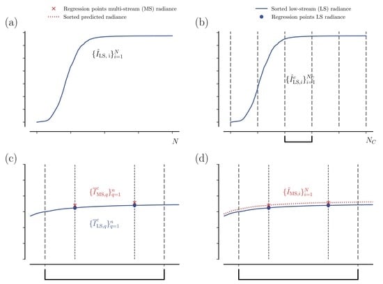
Remotesensing 12 01250 g003
Figure 4. Scheme of the Cluster Low-Streams Regression (CLSR) method. (a) Sorted radiance of the low-stream (LS) model in ascending order (blue line). (b) Division of the LS radiance in equal clusters C in the sorted domain. (c) Zoom for one cluster and the selected regression points of the multi-stream (MS) radiance (red crosses). (d) Reconstruction of the MS spectra: the predicted radiance is computed for all the spectral points (dashed red line).
Remotesensing 12 01250 g004
Figure 5. Radiance spectra computed by using the multi-stream RTM for three atmospheric scenarios: ‘Clear sky’ (black), ‘Cloud 1’ (purple) and ‘Cloud 2’ (blue). The upper panel corresponds to the O2 A-band, while the bottom panel is for the CO2 weak band.
Remotesensing 12 01250 g005
Figure 6. Box plots of the residuals with respect to the continuum in percentage for (upper panels) the PCA model and (bottom panels) the CLSR method, when the low-stream model is (a) the two-stream model for the ‘Cloud 2’ scenario or (b) the single-scattering model for the ‘Aerosol 2’ scenario. The red boxes indicate the O2 A-band while the blue boxes indicate the CO2 band. Box description: the upper and lower limits of the box represent the interquartile range (IQR), which is ( Q 3 Q 1 ) being Q i the i-th quartile; the upper and lower whiskers indicate ( Q 3 + 1.5 · IQR) and ( Q 1 1.5 · IQR), respectively; the orange line inside the box represents the median; the orange values on top of each box indicate the median values and the black values correspond to the IQR value.
Remotesensing 12 01250 g006
Figure 7. Explained variance ratio in percentage as a function of the number of PCs for all the atmospheric scenarios: ‘Clear sky’, ‘Aerosol 1’, ‘Aerosol 2’, ‘Cloud 1’ and ‘Cloud 2’; and the two spectral bands (O2 A- and CO2 bands). The red color corresponds to the O2 A-band and the blue color to the CO2 weak band. The different dashing of the lines indicates the different atmospheric scenarios.
Remotesensing 12 01250 g007
Figure 8. Dependence of the number of clusters and number of regression points with the mean error in percentage for the CO2 band for the ‘Aerosol 2’ scenario. The low-stream model used is the two-stream model.
Remotesensing 12 01250 g008
Figure 9. Comparison of the residuals for the methods PCA and CLSR for all the atmospheric scenarios (grey: ‘Clear sky’; blue: ‘Aerosol 1’; red: ‘Aerosol 2’; green: ‘Cloud 1’; yellow: ‘Cloud 2’) and gases (O2 A- and CO2 bands), when the low-stream model is (a) the two-stream model or (b) the single-scattering model. Note the differences in scales for the PCA technique for the O2 A-band with the rest of cases. The orange values on top of each box indicate the median values and the black values correspond to the IQR value.
Remotesensing 12 01250 g009
Figure 10. Convolved spectra for the multi-stream model and the two acceleration methods for the ‘Cloud 1’ scenario using PCA and CLSR methods for the sensors GOME-2, TROPOMI and GOSAT. For GOME-2 and TROPOMI the O2 A-band spectra are convolved, while for GOSAT the CO2 spectra are convolved.
Remotesensing 12 01250 g010
Table 1. Aerosol optical thickness used in the simulations for O2 A- and CO2 bands at the middle of the corresponding absorption band.
O2 A-Band (760 nm)CO2 Band (1610 nm)
Aerosol 10.20.08
Aerosol 21.20.41
Table 2. Mean relative error ε for the low-stream models (single-scattering and two-stream models) compared with the multi-stream model for the O2 A-band.
ScenarioSingle-Scattering ModelTwo-Stream Model
ε (%) ε (%)
Clear sky3.40.14
Aerosol 1361.0
Aerosol 2784.6
Cloud 1937.1
Cloud 2931.4
Table 3. Mean relative error ε for the low-stream models (single-scattering and two-stream models) compared with the multi-stream model for the CO2 weak band.
ScenarioSingle-Scattering ModelTwo-Stream Model
ε (%) ε (%)
Clear sky0.2030.004
Aerosol 114.70.40
Aerosol 255.52.1
Cloud 197.566.13
Cloud 297.912.00
Table 4. Computational time in seconds of the radiative transfer solution as a function of the number of streams, and speedup factors with respect to the case N do = 32 .
N do Time (s)Speedup Factor
00.45800
13.2725
212.4187.1
434.467.4
811021
165504.2
322320-
Table 5. Speedup factor of the PCA-based ( S PCA ) and CLSR methods with: the two-stream model ( S CLSR TS ) and single-scattering model ( S CLSR SS ).
S PCA S CLSR TS S CLSR SS
5345051294
Table 6. Spectral ranges and FWHM of the Gaussian slit functions of the instruments used in the study: TROPOMI, GOME-2 and GOSAT.
InstrumentSpectral RangeFWHM
TROPOMI710–775 nm0.183 nm
GOME-2590–790 nm0.51 nm
GOSAT1.56–1.69 µm0.2 cm−1
Table 7. Mean relative error ε for the convolved spectra compared with the multi-stream spectra for the PCA-based and CLSR methods and for the different atmospheric scenarios considered for the O2 A-band. In all cases, the low-stream model considered is the two-stream model. The instruments analyzed are GOME-2 and TROPOMI, which are compared with the non-convolved values.
ScenarioO2 A-Band
GOME-2TROPOMINon-Convolved
ε PCA ( % ) ε CLSR ( % ) ε PCA ( % ) ε CLSR ( % ) ε PCA ( % ) ε CLSR ( % )
Clear sky0.0210.0040.0210.0040.0220.006
Aerosol 10.0490.0070.0500.0070.0610.011
Aerosol 20.8370.0190.8370.0190.8560.026
Cloud 11.230.0111.230.0111.240.017
Cloud 22.920.0062.920.0062.930.009
Table 8. Mean relative error ε for the convolved spectra compared with the multi-stream spectra for the PCA-based and CLSR methods and for the different atmospheric scenarios considered for the CO2 band. In all cases, the low-stream model considered is the two-stream model. The instrument analyzed is GOSAT, which is compared with the non-convolved values.
ScenarioCO2 Band
GOSATNon-Convolved
ε PCA ( % ) ε CLSR ( % ) ε PCA ( % ) ε CLSR ( % )
Clear sky0.00030.00030.00060.0006
Aerosol 10.00750.00670.0100.012
Aerosol 20.0350.0120.0440.017
Cloud 10.0110.0070.0130.008
Cloud 20.0110.0050.0160.006

